Dynamic pricing and inventory control with no backorders under uncertainty and competition

Dynamic Pricing and Inventory Control with no

Backorders under Uncertainty and Competition

by

Elodie Adida

Submitted to the Sloan School of Management

in partial fulfillment of the requirements for the degree of

Doctor of Philosophy in Operations Research

at the

MASSACHUSETTS INSTITUTE OF TECHNOLOGY

June 2006

©

Massachusetts Institute of Technology 2006. All rights reserved.

Author ...

...

Sloan School of Management

May 18, 2006

Certified

by...

Georgia Perakis

J. Spencer Standish Associate Professor of Operations Research

Thesis Supervisor

Aiccepted

by ... ... ... ... ... ...

James B. Orlin

Edward Pennell Brooks Professor of Operations Research

Codirector, Operations Research Center

MASSACHUSMlS

_IOFECHNOLOGY

I

j~~

Dynamic Pricing and Inventory Control with no Backorders

under Uncertainty and Competition

by

Elodie Adida

Submitted to the Sloan School of Management on May 18, 2006, in partial fulfillment of the

requirements for the degree of

Doctor of Philosophy in Operations Research

Abstract

Recently, revenue management has become popular in many industries such as the airline, the supply chain, and the transportation industry. Decision makers realize that even small improvements in their operations can have a significant impact on their profits. Nevertheless, determining pricing and inventory optimal policies in more realistic settings may not be a tractable task. Ignoring the potential inaccuracy of parameters may lead to a solution that actually performs poorly, or even that vi-olates some constraints. Finally, competitors impact a supplier's best strategy by influencing her demand, revenues, and field of possible actions. Taking a game the-oretic approach and determining the equilibrium of the system can help understand

its state in the long run.

This thesis presents a continuous time optimal control model for studying a dy-namic pricing and inventory control problem in a make-to-stock manufacturing sys-tem. We consider a multi-product capacitated, dynamic setting. We introduce a demand-based model with convex costs. A key part of the model is that no backo-rders are allowed, as this introduces a constraint on the state variables. We first study the deterministic version of this problem. We introduce and study a solution method that enables to compute the optimal solution on a finite time horizon in a monopoly setting. Our results illustrate the role of capacity and the effects of the dynamic nature of demand. We then introduce an additive model of demand uncertainty. We use a robust optimization approach to protect the solution against data uncertainty in a tractable manner, and without imposing stringent assumptions on available in-formation. We show that the robust formulation is of the same order of complexity as the deterministic problem and demonstrate how to adapt solution method. Fi-nally, we consider a duopoly setting and use a more general model of additive and multiplicative demand uncertainty. We formulate the robust problem as a coupled constraint differential game. Using a quasi-variational inequality reformulation, we prove the existence of Nash equilibria in continuous time and study issues of unique-ness. Finally, we introduce a relaxation-type algorithm and prove its convergence to

a particular Nash equilibrium (normalized Nash equilibrium) in discrete time. Thesis Supervisor: Georgia Perakis

Acknowledgments

First, I would like to thank my understanding family for their support throughout my studies: my brother and sister, Arieh and Sarah, as well as my mother, who dedicated her life to her children.

I would also like to thank my fellow ORC students, with whom I shared many hours studying in the Operations Research Center on tests, qualifying exams, prob-lem sets and research, and who were ready to help out on anything from research problems to changing apartments and debugging a java code: Susan, Michele, Carol, Lincoln, Victor, Mike, Anshul, David, Ping, Jeff, Soulaymane, Dessi who was my e-pal, Guillaume, Carine, Tim, and Th6o.

Moreover, I am very grateful to the Professors on my thesis committee besides my advisor: Prof. Dimitris Bertsimas and Prof. Jremie Gallien. Their feedback was extremely helpful to improving my thesis, suggesting new directions of research, and providing a new perspective on my work.

Finally, I want to thank my research advisor, Prof. Georgia Perakis. It is difficult to fully acknowledge here the extent of her support and express my gratitude. For the last four years, she has shown incredible support and patience, believing in me more than I ever believed in myself. I doubt I would have reached this point today without her consistent mentoring, help and advice. Even academically, her involvement went way beyond research advising. But the most amazing aspect is how she genuinely cares about her students personally. This last year, she helped far beyond what one would expect from an advisor during my job search. I could tell how important it was to her, and her advice was crucial to my decision-making. Most of all, I always appreciated her honesty. There was never need to second-guess her, and I could trust that she would only say what she thought, whether it was positive or negative. As a result, I knew her feedback was sincere, and in return, I felt free to speak openly, which was invaluable. Over the years, she became more a mentor and a friend than simply an advisor. I have no doubt that she will continue to support me throughout my career and knowing this makes the transition much easier.

Contents

1 Introduction

1.1 Motivation .

1.1.1 Dynamic nature of the problem 1.1.2 Uncertainty.

1.1.3 Competition . 1.2 Literature review.

1.2.1 Dynamic pricing, inventory control, ply chain, and optimal control . . . 1.2.2 Demand uncertainty.

1.2.3 Competition .

...

1.3 Overall goal and structure of the thesis . .

. . .. . . .. . . .. . . .. . . .. revenue . . .. . . .. . . .. . . .. . oo .o. .. .. management, sue . . . .. . . . . ... . . . . . . .. . . . . . . . . . .. . . . . . . . . .. 2 Formulation 2.1 Modeling assumptions ...

2.1.1 No backorders constraint on inventory levels 2.1.2 Capacity constraint.

2.1.3 Cost structure .

2.2 Demand model in a deterministic monopoly setting 2.3 Uncertainty model in a monopoly setting ...

2.3.1 An additive model ... 2.3.2 Budget of uncertainty.

2.4 Model in a duopoly setting ...

2.4.1 Formulation . . . . 17 18 19 21 22 23 23 27 29 31

33

>-2.4.2 Demand model . . . .

2.4.3 Budget of uncertainty ... 2.5 Objective function under uncertainty ... 2.6 Notations ...

2.6.1 Monopolistic and deterministic setting ...

2.6.2 Additional notations for the monopolistic setting with uncertainty 2.6.3 Notations for the duopolistic setting with uncertainty ...

3 Deterministic and monopolistic setting

3.1 Definitions, formulation, and description of 3.1.1 Description of the model ... 3.1.2 Existence of an optimal solution . . 3.1.3 Solution approach .

3.2 Maximum Principle . 3.2.1 Theoretical results.

3.2.2 Necessary conditions for optimality 3.3 Derivation of the solution method ...

the solt

3.3.1 The optimal policy as a function of the multipliers

variables

...

3.3.2 First step: (qi + pi)(t), i = 1,...,

N are known

57 ition approach . . 57 ... ...58 ... ...60 ... ...65 ... ...67 ... ...67 ... ...71 ... ...77 and adjoint 77 79

3.3.3 Second step: the system is observable at each time t ... 3.3.4 Third step: No external information is given ... 3.4 Algorithm ...

3.5 Computational results and insights ...

3.5.1 Example 1: Impact of a demand peak and of the capacity

con-straint.

3.5.2 Example 2: Impact of constant price sensitivities (coefficients

/,i(.)) with a demand peak ...

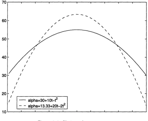
3.5.3 Example 3: Impact of time-varying price sensitivities (coeffi-cients i(.)) with a constant maximum demand ...

45 49 50 51 52 54 54 85 101 115 125 125 133 134 . . . .

4 Uncertain data in a monopoly setting: a robust optimization

ap-proach

4.1 Derivation of the robust counterpart problem ... 4.1.1 Equivalent deterministic formulation ... 4.1.2 Solution of the dual subproblem ... 4.1.3 Properties.

4.1.4 Robust counterpart problem ...

4.2 Traditional worst-case objective robust counterpart ...

4.3 Solving the robust counterpart problem ...

4.4 Numerical results.

4.4.1 Choice of parameters.

4.4.2 Closed-form solution for the dual subproblem (4.7)

4.4.3 Results .

...

5 Uncertain data in a duopoly setting

165

5.1 Duopoly setting with deterministic data . ... 166

5.1.1 Formulation ... 166

5.1.2 Definitions and properties . . . 168

5.1.3 Quasi-variational inequality formulation ... 174

5.1.4 Existence of a Nash equilibrium ... 177

5.2 Duopoly setting with uncertain data . ... 181

5.2.1 Robust counterpart problem ... 181

5.2.2 Properties of the minimum inventory security level ... 187

5.2.3 Existence of a Nash equilibrium ... 190

5.3 Formulation in discrete time with uncertain data ... 198

5.3.1 Formulation and properties ... 198

5.3.2 Nash equilibria ... 205

5.3.3 Normalized Nash equilibrium . . . ... 208

5.3.4 Uniqueness results ... 226

5.4.1 Description of the algorithm ... 232

5.4.2 Theorem of convergence ... .. 234

5.4.3 Continuity of the best response function ... 235

5.4.4 Weak convexity with respect to the first argument ... 236

5.4.5 Concavity with respect to the second argument ... 237

5.4.6 An inequality ... 239

5.5 Numerical results ... 241

5.5.1 Deterministic model ... 241

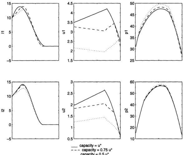
5.5.2 Effect of the price sensitivities ... 242

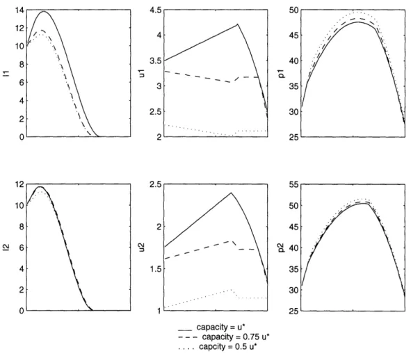
5.5.3 Effect of capacity . . . ... 247

5.5.4 Effect of initial inventory level ... 250

5.5.5 Robust formulation ... 253

List of Figures

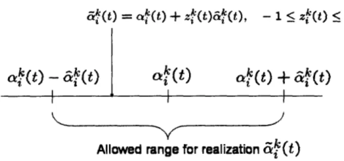
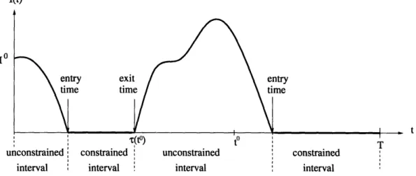
2-1 Uncertainty model: illustration for &i(t) ... 2-2 Uncertainty model: illustration for & (t) ... 3-1 Example of evolution of the inventory level ...

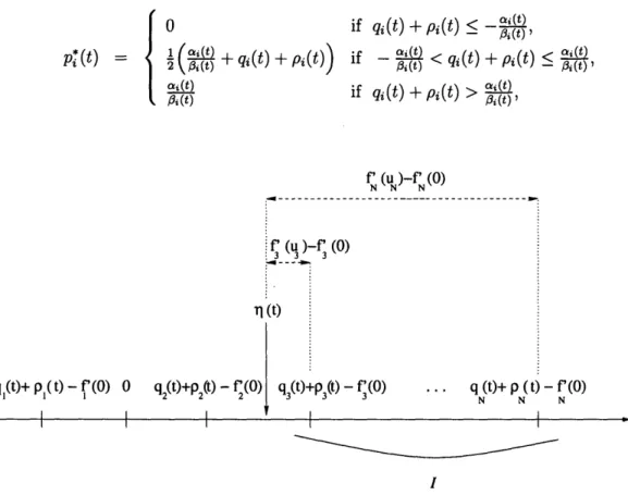
3-2 Algorithm Al(t): Example with q(t) > 0, when products 3,..., N are active.

3-3 Algorithm A2(t): Example with > 0, when products 3, ... N are

active at time t. In particular, products 1 and 3 are unconstrained and

3-4 3-5 3-6 3-7 3-8 3-9

products 2 and N are constrained.. Choices of parameters a ... Solution for demand scenario 1 . . Solution for demand scenario 2 . . Solution for demand scenario 3 . . Solution for price sensitivities equal Solution for price sensitivities equal

to .1 to 1 to 1

... . .92

4-2 Choice of budget uncertainty function F(.)... 4-3 Optimal inventory levels over time results .... 4-4 Optimal production rates over time results .... 4-5 Optimal prices over time results ...

4-6 Trade-off between robustness and performance . . 5-1 Example 1 in the space of prices: set Q(p*A,p*B) ).

157 158 160 160 161 163 203 41 48 58 81

5-2 Example 1 in the space of prices: set Y ... 204

5-3 Example 2: illustration of jointly feasible set, set unstable under the best response function, Nash equilibria, system optimum, normalized

Nash equilibrium, and Pareto optimal points ... 216

5-4 Modified example in space of prices: set Q(p*A, p*B) ... . 229

5-5 Modified example in space of prices: set Y ... 230

5-6 Results: Effect of price sensitivities. Equilibrium in the case of price

sensitivities increasing with time ... .. 244

5-7 Results: Effect of price sensitivities. Equilibrium in the case of price

sensitivities decreasing with time ... . 245

5-8 Results: Effect of production capacity. Equilibrium in the case of

scenario f for various symmetric capacity levels ... 248

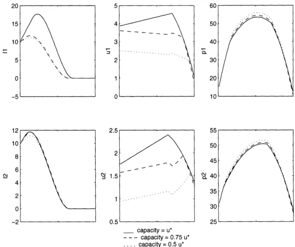
5-9 Results: Effect of production capacity. Equilibrium in the case of

scenario h for various symmetric capacity levels ... 249

5-10 Results: Effect of initial inventory level. Equilibrium in the case of

scenario f for various initial inventory levels ... 251

5-11 Results: Effect of initial inventory level. Equilibrium in the case of

scenario h for various initial inventory levels ... 252

5-12 Results: Robust formulation. Equilibrium in the case of price sensitiv-ities scenario f for various scenarios of budget of uncertainty ... 255 5-13 Results: Robust formulation. Equilibrium in the case of price

sensitiv-ities scenario h for various scenarios of budget of uncertainty ... 256 5-14 Results: Total objective value of the equilibrium under scenario f as a

function of the cumulative effective budget of uncertainty ... 259 5-15 Results: Total objective value of the equilibrium under scenario h as a

function of the cumulative effective budget of uncertainty ... 259 5-16 Example of realizations for alpha under uniform and normal distributions260 5-17 Histogram of minimum inventory level reached for uniformly distributed

5-18 Histogram of minimum inventory level reached for uniformly distributed

realization in scenario h ... 263

5-19 Histogram of minimum inventory level reached for normally distributed

realization in scenario f ... 264

5-20 Histogram of minimum inventory level reached for normally distributed

List of Tables

3.1 Choice of input parameters in the deterministic, monopoly setting . 125

3.2 Scenarios of evolution of parameter a(t) . ... 126

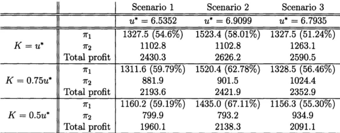
3.3 Numerical results: Profits under different scenarios. 7ri denotes the profits due to product i. ... 131

4.1 Data chosen as input in the numerical implementation for the robust formulation ... 157

4.2 Multiple scenarios of budget of uncertainty . ... 159

4.3 Objective value results ... 162

5.1 Prisoner's dilemma penalties: first case . ... 214

5.2 Prisoner's dilemma penalties: second case . . . ... 214

5.3 Scenarios of price sensitivities . ... 243

5.4 Objective values: effect of price sensitivities . ... 246

5.5 Results: Effect of production capacity. Profits for various symmetric capacity levels . . . ... 247

5.6 Results: Effect of initial inventory level. Profits for various symmetric initial inventory levels ... . 250

5.7 Total objective value for various budgets of uncertainty ... 258

5.8 Probability of violation of the no backorders constraint for the nominal solution ... 261

5.9 Probability of violation of the no backorders constraint for the robust solution ... 262

Chapter 1

Introduction

The profitability of operations of a firm is critically affected by decisions regarding its pricing, inventory and production strategy. Static policies usually perform poorly compared to dynamic policies, in which the price and production rate are adjusted over time. Indeed, the demand in particular, and sometimes other components of the system, usually evolve over time. Today, many channels of distribution (such as the internet) allow suppliers to change prices over time when they can benefit from a dynamic strategy. A dynamic strategy requires the price and production rate to be determined at all times in order to maximize the net profit over a time horizon, while obeying some constraints due to stock level limits or production capacity, taking into account production and inventory holding costs. Moreover, when the firm produces simultaneously multiple products, new decisions must be made to allocate the avail-able production capacity among the products.

Practitioners often face the problem of uncertainty when determining model rameters. Ignoring uncertainties may yield a strategy that is useless if the true pa-rameter values differ from their model estimate. Indeed, this strategy may not only be very suboptimal, but may also be infeasible due to constraint violations. It is there-fore of great importance to provide a way to incorporate uncertainty in the model, while proposing tractable solutions, and without making unrealistic assumptions.

We consider an oligopoly market with differentiated products, where multiple

competitors target the same potential buyers. In such a setting, the price of a

prod-uct at a given firm affects the demand of all firms for that prodprod-uct. In other words, the demand observed by a given firm for some product depends not only on her own price, but also on the prices applied by her competitors. Therefore, each competitor has to determine her strategy based on her competitors' prices. To understand how competition affects optimal decisions, we place the problem within a game-theoretic

setting and study equilibria.

The overall goal of this research is to provide a model of dynamic pricing and in-ventory management under demand uncertainty and competition, when no stock-outs are allowed. We are facing contradicting challenges, since we wish to build a model as realistic as possible but at the same time to gain insights from its solution in or-der to reach a better unor-derstanding of how to determine optimal strategies in practice.

1.1 Motivation

Recently, revenue management has become popular in many industries such as the airline, the supply chain, and the transportation industry. Many retail firms have rec-ognized that better revenue management and inventory control may yield significant positive impact. They invest time and effort in an attempt to optimize their prices and inventory policies. One of the critical factors to determine the profitability of a firm is its pricing and production strategy. Many firms hire specialized consultants to help them determine optimal strategies and improve their revenue management. A study by McKinsey and Company on the cost structure of Fortune 1000 companies in the year 2001 shows that pricing is a more powerful lever than variable cost, fixed cost or sales volume improvements. An improvement of 1% in pricing yields an average of 8.6% in operating margin improvement (see [10]). Therefore, companies' ability to survive in a competitive environment depends on the development of efficient pricing

models. Inventory control can also have a major impact on profits. Abernathy et al. note that "Retailers no longer place large seasonal orders for goods in advance instead, they require ongoing replenishment of stock, forcing manufacturers to predict demand and then hold substantial inventories indefinitely. Manufacturers now carry the cost of inventory risk. (...) The inventory demand for stock-keeping units within the same product line can vary significantly. (...) By differentiating inventory policies at the stock-keeping unit level, manufacturers (...) improve the profitability of the entire line." [1]. As a result, dynamic pricing, inventory control and revenue manage-ment have become very active research topics and have been extensively studied in the academic literature in Economics, Operations Management, and Marketing (see for example [34], [57], [119], [130]). In such settings, suppliers are maximizing their profits over a time horizon subject to some constraints. Furthermore, data changes over time. Therefore, these problems are typically formulated as constrained dy-namic optimization problems. Dydy-namic Pricing and Inventory Control problems are challenging due to various aspects of the problem:

(a) the intrinsically dynamic aspect; (b) uncertainty of the demand;

(c) competition among suppliers;

(d) the non separability of the decision variables (prices and production decisions are typically inter-dependent).

1.1.1 Dynamic nature of the problem

In a setting where parameters and decision variables change over time, the state of the system constantly evolves. In particular, the inventory level is variable that rep-resents the current state of the system. It results from the initial state and the entire history of decisions until the current time. In an open-loop framework, the value of data over time is known in advance, and decision makers commit at time zero to their decision over the time horizon, in order to maximize the total profits. In such a

framework, the solution is determined by considering the entire time horizon, rather than by taking a myopic approach that would seek to maximize the instantaneous profits. It is important to realize that the decisions at a given time have an impact on the future state of the system. For example, if the demand is expected to increase over time, and production capacity is small, it may be optimal to choose a high pro-duction rate even at the beginning of the horizon even though the low demand at the time does not require it, in order to build up inventory stock. Then it will be possible to satisfy the high demand later on without increasing prices. Otherwise, the low production capacity would not have been sufficient to satisfy the demand, and prices would have to increase in order to slow demand. This example illustrates how optimal decisions are linked over time. Therefore, the dynamic aspect of the problem is essential for determining its optimal solution.

To model the dynamics of the system, some researchers choose to view time as discrete. The drawback of such an approach is having to decide the length of the step size. A fine discretization of the time horizon provides more accuracy. Nevertheless, it gives rise to a problem of a huge size, both in terms of number of variables and number of constraints (even though the dimension is finite), which implies significant delays in obtaining good solutions. When viewing time continuously, the inventory may be seen as a continuous flow, and as a result, there is no need to assume that decisions occur only at discrete points on the time axis. The problem can be formu-lated as a fluid model. Fluid models provide a powerful tool for understanding the behavior of systems where the dynamic aspect plays an important role. They arise in applications as diverse as routing, communication, queueing, supply chain and trans-portation systems. They have been used in particular as approximations of complex stochastic systems, such as queueing networks. Recent research has proven that an attractive feature of these models in supply chain applications is that they provide good scheduling, production and inventory policies in a variety of settings. Moreover, fluid models allow a continuous time approach instead of having to discretize time. However, since demand depends on prices, these formulations are nonlinear, and as

such, may be very complex to solve. Examples of supply chain industries where fluid models of the type we discuss in this thesis are relevant, include industries with a high volume of throughput and data on costs and demand that change a lot. The hardware as well as the semiconductor industries are such examples. Moreover, we believe that a similar approach can be applied to problems in areas other than dynamic pricing and inventory control, where the dynamic evolution of the system justifies a contin-uous time approach. We believe that the techniques presented in this thesis may be helpful to those areas as well.

1.1.2 Uncertainty

Most of the time, practitioners and researchers assume that their model represents well reality, and that data are known with certainty. However, uncertainty is inherent in nature and forecasts always involve some degree of randomness since many unex-pected events may affect the future. Moreover, the model may inexactly represent the system and the interactions between its components. For instance, modeling the demand as varying linearly with the price, is an approximation of the true relation-ship between price and demand. Finally, even when the model is exact, its validity relies on the ability to determine the exact values of its parameters, which may be difficult to measure in practice. One way to evaluate those parameters is the use of regression or statistical inference models based on historical data. Nevertheless, these methods provide only an estimate of the parameters. Furthermore, they are based on the assumption that the future can be inferred from the past, and this assumption is not always justified. Ignoring the potential inaccuracy of models parameters may lead to a solution that performs poorly if the actual value differed from the one assumed in the model, or even that is infeasible. In particular, when in the nominal model constraints are binding at this solution, it is likely that even a small perturbation of the data will yield a violation of those constraints.

A common approach to address uncertainty is to assume a probability distribu-tion on the parameters, and use stochastic optimizadistribu-tion and dynamic programming.

However, suppliers may find it difficult in practice to determine such probability dis-tributions. In most applications, it may be unrealistic to know anything other than the first and second moment of the distribution. For reasons mentioned above, even historical data may not be sufficient to have an accurate idea of the probability dis-tribution. Moreover, even if the distribution is known, solving these formulations is often not possible because of what is known as the "curse of dimensionality". As the number of periods increases, the dimension of the problem is so large that the problem becomes intractable.

This idea motivates a robust optimization approach. The main idea is to find the best strategy given some uncertainty model on the data. The field of robust optimiza-tion has attracted a lot of research recently by providing an efficient way of finding good solutions that are immune (or robust) to data uncertainty. Robust optimiza-tion is also easier to use than stochastic optimizaoptimiza-tion and dynamic programming in practice because it does not require to make any assumption on the probability dis-tributions: it only requires a range of variation, which is not very difficult to estimate in most applications. We will consider that the demand parameters are subject to uncertainty, since they are the most difficult to evaluate in practice. The tractability of solving the problem under this approach depends essentially on the structure of the uncertainty set within which the data are allowed to vary. Part of the task in formulating the robust model is to design these sets in such a way that tractability

is preserved.

1.1.3 Competition

A third important feature we would like to study is competition. In a non-monopolistic setting, several firms compete. The decisions taken by a firm may affect other firms by influencing her demand, revenues, and field of possible actions. Thus when multi-ple sellers compete in a market, these mutual interactions motivate a game theoretic approach which makes a key difference in the techniques determining the solution. Such problems have been studied in the literature in economics, revenue management,

and supply chain.

There are many ways of modeling competition based on the number of competi-tors, whether there is a leader and some followers, whether competitors cooperate, etc. In this thesis, we assume an oligopoly where all suppliers simultaneously seek to optimize their revenues. The question of interest is then to determine if the game has an equilibrium, i.e. a solution for all competitors such that no one has an incentive to unilaterally deviate from it (Nash equilibrium). For most settings, it would be un-realistic to assume a monopoly or that competitors cooperate. Oligopolistic settings with no collaboration are thought to protect the customer by guaranteeing fair prices due to the competition between suppliers. Most developed economies have laws that prohibit monopolies and cooperation (US Antitrust law for example). Therefore, in this thesis we will consider a non cooperative oligopolistic competition.

1.2 Literature review

In this section, we provide an overview of the literature on topics closely related to the thesis. We first discuss some related papers on revenue management, dynamic pricing and optimal control in a monopoly setting. Then we present references that are relevant to modeling demand uncertainty. Finally, we mention literature relative to oligopolistic competition.

1.2.1

Dynamic pricing, inventory control, revenue

manage-ment, supply chain, and optimal control

There is a huge literature on inventory control as well as pricing and revenue manage-ment. For example, the book by Porteus [108] and the book by Zipkin [130] review inventory management techniques, while the book by Talluri and van Ryzin [119] pro-vides an overview of the revenue management and pricing literature. In this section,

we provide details and references on advances in areas related to different aspects of

the thesis.

In a setting where the problem has a dynamic aspect, such as traffic control, queueing networks, supply chain, or transportation, there is a connection with fluid models. These models can be viewed (when there is no stochasticity) as continuous time optimal control models. A large part of the literature on continuous-time opti-mal control models has focused on the solution of linear formulations (see for example Anderson [4], [5], Pullan [109]). This part of the literature shows existence of an op-timal solution with piecewise constant controls. Pullan in particular showed strong duality and designed a class of algorithms solution convergent. For the solution of linear fluid models, Bertsimas and Luo [93] construct an algorithm solving state con-strained separated continuous linear programs under some assumptions. Fluid models also connect with semi-infinite programming problems. Tuncel and Todd [121] study the asymptotic behavior of interior point methods for semi-infinite programming by finding the limits of search directions, potential functions and central paths as the number of variables becomes infinite.

However, when fluid models are nonlinear, the dynamic together with the nonlinear aspect of the problem make them harder to analyze. Nonlinear fluid models are par-ticularly useful for dynamic pricing and inventory management applications, as we explained above. A variety of models have been proposed in the literature for such applications (see references below). These models typically differ due to the produc-tion cost, inventory cost, and demand funcproduc-tions considered. More theoretically, many papers study general continuous time optimal control models. [7], [73], [85] and [115] give formulations of the Maximum Principle under state variable constraints. Clarke ([43], [44], [45], [46] with others) and Devdariani and Ledyaev [51] provide theoretical results on global optimality conditions.

The literature on dynamic pricing is growing fast. Elmaghraby and Keskinocak in [57] and the references therein provide a comprehensive literature review of dynamic

pricing models while Bitran and Caldentey [34] provide an overview of research on dynamic pricing and its relation to Revenue Management. Furthermore, Zipkin [130] and the references therein provide a thorough review of recent advances in inventory control theory and its relation to supply chain. Chan, Shen, Simchi-Levi and Swann [39] review research on coordination of pricing and inventory decisions. Finally, Yano and Gilbert [126] and the references therein provide a review of pricing and produc-tion/procurement decisions.

A large volume of literature studies a demand model for the single-product case. For example Pekelman [105] solves the dynamic pricing and production policy prob-lem for a single product optimizing over a finite time horizon. He models the demand as a linear function of the price with time-varying coefficients. The model uses linear inventory cost with a constant coefficient, and a general strictly convex production cost. The model does not allow backorders (negative inventory levels). Feichtinger and Hartl [60] extend this model by considering a general nonlinear demand function and allowing backorders, with both piecewise linear and strictly convex inventory costs. They obtain phase diagrams for the equilibrium and transient behavior of the optimal solution with a finite or infinite time horizon. Another extension is intro-duced by Thompson, Sethi and Teng in [120], where the production rate and the level of inventory are bounded, and the production cost is either linear or strictly convex. Gaimon [64] considers additional controls by allowing decisions on the max-imal production rate as well as price and production output, where the change in maximal production rate has an effect on the production cost. [56], [78] and [89] consider the case of centralized or decentralized decisions between a distributor and a manufacturer in an industrial channel of distribution. Locke Anderson [91] con-siders production decisions when the production of a final good requires as input the production of an intermediate good. In the single-product model, Jrgensen [79] uses a continuous time optimal control model to study demand learning effects while Laurent-Varin [90] introduces an interior-point solution algorithm.

In a multi-product setting, Bertsimas and Paschalidis [28], Harrison [72] and Meyn [98] study a make-to-stock problem using fluids. Specifically, Bertsimas and Pascha-lidis in [28] study an inventory control problem with fixed demand rate and capacity rate shared among all classes. Their model allows backorders and computes a produc-tion policy by minimizing either a linear or a quadratic inventory cost over successive small intervals. Luo [92] considers a make-to-stock multi-class queueing scheduling problem that minimizes a convex quadratic backorder and holding cost and finds an optimal production policy over the entire time horizon. Kleywegt [86] uses a cutting plane algorithm to solve a multi-class optimal control problem of dynamic pricing with profit linear in terms of selling rate. Fleisher and Sethuraman [62] provide an approximation algorithm to solve the optimal control of fluid queueing networks. Moreover, van Ryzin and McGill [124] designed an adaptive approach within the framework of airline revenue management based on historical observed data. They study an algorithm through stochastic approximation theory. Gallego and van Ryzin [66], [67] consider the problem of dynamically pricing over a finite horizon when de-mand is stochastic and price sensitive. Finally, Kachani and Perakis [82], [83] take a delay-based approach to determine optimal pricing and production policies, where the price and level of inventory affect the delay (time that a product remains in inventory).

A stream of research has focused on a dynamic programming approach to solve pricing and/or inventory problems (see [2], [26]), by dividing the (possibly infinite) time horizon into time periodsand allowing decisions at the beginning of each period, as opposed to the research cited above that takes a continuous approach, including Maglaras and Meissner [95] who approach the pricing problem under fixed capacity by reducing the problem to determining the aggregate rate at which all products jointly consume resource capacity, and defining an efficient frontier.

1.2.2 Demand uncertainty

Economists have used a variety of demand models which have been applied in the revenue management literature (see for example, [6], [125], survey articles [39] and [57]). The problem of demand uncertainty has motivated a significant amount of literature in the field of Revenue Management and Pricing. A number of different

approaches have been introduced to model this uncertainty. Zabel [129] considers two models of uncertain demand: a multiplicative model (dt = rtu(pt)) and an ad-ditive model (dt = u(pt) + t), where dt is the demand at time t, pt is the price at time t, u(p) = a - p, i.e. a downward sloping linear demand curve, and t is

assumed to be either exponentially or uniformly distributed with E[vt] > 0. Young [128] and Federgruen and Heching [58] generalize the demand model to be of the form dt = yt(p)et + t(p), where -y and 6 have first derivatives non positive and et is a random term with a finite mean. Gallego and van Ryzin [66], [67] as well as Bitran and Mondschein [35] assume that demand follows a Poisson process with a deterministic intensity that depends on price and time. Raman and Chatterjee [110] model the stochasticity of the demand by introducing an additive model where the random noise is a continuous time Wiener process.

For additional details and references, see review papers such as [34], [57] and [126].

The Operations Research literature treats the presence of data uncertainty in op-timization problem in several ways. The problem is sometimes solved assuming all parameters are deterministic; subsequently sensitivity analysis is performed to study the stability of the nominal solution with respect to small perturbations of the data. Stochastic programming is used when a probability distribution of the underlying uncertain parameters is available, and seeks a solution that performs well and has low probability of constraint violation. Robust optimization is an alternative was to seek an optimal solution of a problem when its data is uncertain.

A robust optimization formulation was first considered by Soyster [117] in the case of a linear optimization problem where the data were uncertain within a convex set.

He addresses uncertainty by taking a worst-case approach. Nevertheless, such an approach decreases the performance of the solution significantly, and was criticized of being overly conservative. Ben-Tal and Nemirovski ([16],[17]) address the issue of over-conservativeness by considering data uncertainty sets that are ellipsoids, for linear programming (LP) and general convex programming. Numerical examples of their approach for polyhedral uncertainty sets, that allow to reformulate the robust counterpart of an LP as an LP, can be found in [18]. El-Ghaoui et al ([54], [55]) inde-pendently developed the approach of robust counterpart applied mostly to uncertain semidefinite programming, by adapting ideas from robust control.

They show that the robust counterpart of many convex optimization problems (LPs, second-order cone problems (SOCPs), semidefinite programming programs (SDPs)) with data within ellipsoidal uncertainty sets can be efficiently solved exactly or ap-proximatively by polynomial-time algorithms. However, for this type of uncertainty sets, complexity increases: the robust counterpart of an LP is reformulated as an SOCP, of an SOCP is reformulated as an SDP, and the robust counterpart of an SDP is NP-hard to solve. In [19], Ben-Tal, Nemirovski and Roos approximate the solution of the NP-hard semidefinite robust counterpart of an SOCP with ellipsoidal uncertainty sets with a single explicit semidefinite program.

Bertsimas and Sim [30] seek a model leading to a robust counterpart problem to an LP that is still a linear optimization problem, by introducing the notion of budget of uncertainty to control the level of conservativeness. They studied the tradeoff between robustness of a solution to a linear programming problem and the sub-optimality of the solution. In [29], they use this approach for discrete optimization and network flow problems. Bertsimas, Pachamanova and Sim [27] propose a framework for robust modeling of LPs using uncertainty sets described by an arbitrary norm. Bertsimas and Sim [31] propose a relaxed robust counterpart for general conic optimization problems that preserves the original structure (robust LPS are LPs, robust SOCPs are SOCPs, robust SDPS are SDPs), and provides probability guarantees on the fea-sibility of the solution. Bertsimas and Brown [25] construct uncertainty sets for LPs by taking a coherent risk measure as primitive.

The robust optimization methodology has been applied to a number of areas. Bert-simas and Thiele [32] apply robust optimization principles to inventory theory and supply chain management. In [15], Ben-Tal and Nemirovski use robust optimiza-tion to formulate a robust truss topology design problem as an SDP. Goldfarb and Iyengar [71] apply robust optimization to portfolio selection problems. They intro-duce uncertainty sets that allow to reformulate the robust counterpart problem as an SOCP. Ben-Tal et al [14] take a robust optimization approach for multi-period stochastic operations management problems, and in particular the retailer-supplier flexible commitment problem with uncertain demand.

1.2.3 Competition

In economics, many game-theoretic problems in continuous time are modeled as differ-ential games, i.e. games involving a fluid equation. Jrgensen and Zaccour [80] apply a differential game model to control pollution emission. They consider two neighboring countries who make decisions on emissions and investments in abatement technol-ogy. The dynamics of capital stocks and the stock of pollution are modeled through a fluid equation. They solve in closed form the cooperative problem and the Nash equilibrium problem, and they design an incentive strategy. Miler and de Zeeuw [96] use a differential game to model a problem related to acid rains. Neighboring coun-tries face a trade-off between costs of emission reductions and the damage to the soils.

Literature on oligopolistic competition in the field of pricing and revenue man-agement is emerging fast in recent years. The book by Vives [125] presents a number of pricing models in an oligopoly market. For a survey of joint pricing and produc-tion decisions for inventory control in a supply chain setting, the reader can refer to Chan et al. [41] as well as Cachon and Netessine [36]. A wide range of applications of pricing can be found in the literature in economics, marketing and management science (see for example, Jrgensen and Zaccour [81] and Dockner and others [52], and the references therein). Fudenberg and Tirole [63] review a variety of game theo-retic models for pricing and capacity decisions. Gaimon [65] studies open and closed

loop Nash equilibria for two firms and a single product setting, where the price and capacity are determined to maximize net profits when the acquisition of new technol-ogy reduces the operating cost. For perishable products, Perakis and Sood [106] and Perakis and Nguyen [100] study non cooperative equilibrium policies. Steinberg and Eliashberg [118] study a production and expenditure problem and obtain a dynamic open-loop Nash equilibrium. Feichtinger [59] applies differential games to advertis-ing. He considers two profit-maximizing firms and studies the structure of optimal advertising rates in the Nash equilibrium solution. For a survey of applications of dif-ferential games to management science, see [61]. In many cases in these applications, the equilibrium point is obtained by solving the differential form of the Kuhn-Tucker optimality conditions. Nevertheless, it is not always the case that solving these con-ditions is tractable.

Differential games are useful to model dynamic systems of conflict and cooperation where decisions are made over a time horizon. Ba§ar presents some theoretic results in [11] for non-cooperative dynamic games. Quasi-variational inequality problems were introduced by Bensoussan and Lions [20], [21], [22], motivated by stochastic impulse control problems. Mosco [99] studies topological and order methods to solve this type of problems with implicit constraints and connects these problems with applications to differential games. Quasi-variational inequalities in finite dimension have been studied by several authors such as Yao [127], Pang [101], Pang and Fukushima [102], and Chan and Pang [38]. Cavazzuti and others [37] introduce some relationships between Nash equilibria, variational equilibria and dynamic equilibria for noncooper-ative games without assuming that the dimension is finite. Cubiotti [48] and Cubiotti and Yen [49] prove the existence of solution for generalized quasi-variational inequal-ities in infinite-dimensional normed spaces under some conditions. Pang and Stewart [103] recently introduced differential variational inequalities and illustrated this no-tion in particular for differential games. Using the maximum principle, Schumacher [112] provides an example of a differential variational inequality for a linear quadratic dynamic optimal control problem with state constraints only, and a linear problem

with control constraints.

The degree of interdependency between players' actions impacts directly the dif-ficulty of finding an equilibrium. Rosen [111] extended the literature on finite dimen-sional n-person non-zero sum games by considering games in which the constraints as well as the payoff function depend on the strategy of every player. He called these games coupled constraint games. He showed the existence of an equilibrium under concavity assumptions, and he introduced the notion of normalized Nash equilibrium as a particular Nash equilibrium. He showed uniqueness of a normalized Nash equi-librium under certain assumptions. This type of games have several applications, for example in routing [53], and in environmental economics [75], [76], [88], [87].

Relaxation algorithms provide a powerful tool for finding a Nash Equilibrium when the problem is not tractable enough to solve the necessary conditions. These iterative algorithms rely on averaging the current solution iterate with the solution of the best response problem each player solves. Uryas'ev and Rubinstein [123] and Bazar [11] study the convergence of such algorithms in finite dimensions for finding the equilibria of a non cooperative game for some payoff functions on a closed, com-pact, subset of Rm. Berridge and Krawczyk [24] apply these techniques to games with non linear payoff functions and coupled constraints arising in economics. Krawczyk and Uryas'ev [88] consider similar problems and use steepest-descent step-size con-trol. Contreras et al. [47] illustrates this method for finding equilibria in electricity markets.

1.3 Overall goal and structure of the thesis

The overall goal of this thesis is to introduce and study an optimization problem for dynamic pricing and inventory control with no backorders for a make-to-stock manufacturing system. We proceed as follows:

Deterministic problem in a monopoly setting: We first present the basic model

in a monopoly setting with no uncertainty in the data.

Robust formulation: We then introduce uncertainty in the demand parameters

and take a robust optimization approach.

Robust formulation under competition: We finally add the aspect of compe-tition to the model and address jointly uncertainty of demand in a duopoly competitive setting. Our goal is to study the Nash equilibria of the system. Given the complexity of the problems we consider, it is clearly impossible to ob-tain closed form solutions. Our goal was to avoid making unnecessary approximations and unreasonable assumptions. Moreover, we attempted to find solution algorithms that, under certain assumptions on the data, converge to the desired solution either in finite time, or in infinite time but with good performance in practice. To the best of our knowledge, this is the first research work associating simultaneously optimal pricing and production strategies, fluid models, uncertainty via robust optimization, and competition.

The thesis is structured as follows. Chapter two provides a detailed description of the model of dynamic pricing and inventory control problem we propose, the as-sumptions of the model, and the notations used.

Chapter three describes a solution method for the deterministic problem in a monopoly setting.

Chapter four proposes a robust optimization model to take uncertainty into account. Furthermore, it illustrates the robust formulation is of the same order of "complexity" as the nominal formulation. In particular, we show how to adapt the method from Chapter three to get a robust solution.

Chapter five studies equilibria in continuous time in a duopoly market where demand is deterministic. Subsequently, it extends these results to incorporate uncertain de-mand. Moreover, this chapter studies an algorithm that converges to an equilibrium in discrete time, when demand is uncertain.

Chapter 2

Formulation

Throughout the thesis, we consider a finite time horizon [0, T] and a dynamic setting. We assume that the suppliers produce multiple non-perishable differentiated prod-ucts i = 1,..., N. We assume that these prodprod-ucts share a common resource which yields a production capacity constraint coupling the products together. Our goal is to determine at time zero the optimal pricing and production strategy for all products on the entire time horizon. The solution for prices and production rates is a set of functions of time on the time horizon. Furthermore, the dimension of the problem is infinite. Assuming that sellers are profit-maximizers, an optimal strategy is the strategy providing the highest net profits, given by the sum over time and across products of the demand multiplied by the price, after subtracting the production and inventory costs. We model the production cost either as a strictly convex increasing function, or more particularly as a quadratic function of the production rate. We model the inventory cost either as a linear or a quadratic function of the inventory level. The resulting problem is therefore nonlinear.

Note that all parameters of the problem are time dependent (including the bounds defining feasible ranges when there is uncertainty), thus allowing to model the dy-namic aspect of such problems.

This chapter provides a detailed description of the general setting, assumptions on the data, and the motivation behind modeling assumptions.

2.1 Modeling assumptions

2.1.1 No backorders constraint on inventory levels

Inventory problems may allow or deny backorders, i.e. the possibility of having a negative inventory level. A key aspect of the problem under consideration is the no backorders constraint which ensures that inventory levels remain non negative at all times:

Ii(t) > 0, i= 1,...,N,

tE [0, T],

where T is the time horizon and Ii(t) the inventory level of product i at time t. In a manufacturing system which does not allow backorders and where the demand rate is not external, but determined by a relationship with price, the price can be adjusted so that no demand is actually lost. That is, the price is set so that there is enough available inventory to satisfy the demand, in such a way that the selling rate equals the demand rate. This setting can be justified by the presence of a contract between a supplier and a retailer, or by very high fixed backlog cost. For example, Pekelman [105] studies a problem of optimal pricing and production for a single product with no backorders. Axsiter and Juntti [8] study echelon stock reorder policies with no backorders.

In the fluid model, the inventory level is given as the solution of a first order differential equation involving the production rate and the price in a linear relation. More specifically, the inventory level at a given time t is the difference between the cumulative production and the cumulative demand up to that time t, where the cumulative production depends on all production rate decisions from time zero up to time t, and the cumulative demand depends on all prices applied for that product from time zero up to time t. It is therefore indirectly related to the decision variables. Reversely, constraints such as production capacity and bounds on the prices involve directly and instantaneously the decision variables, and have as a result a simpler impact on the set of feasible strategies. The inventory level at a given time is a

state variable, i.e. it characterizes the state of the system at that time based on all

choices of decisions variables up to that time. The no backorders constraint imposes a non negativity constraint on the inventory levels at each time. Therefore, as a state variable constraint, it is difficult to deal with and makes the problem significantly more complex.

2.1.2 Capacity constraint

We assume that multiple products share a single common production capacity by

introducing the constraint

N

Zui(t) < K(t), Vt E [O,T], i=l

where ui(t) is the production rate of product i at time t and K(t) is the total

produc-tion capacity rate at time t. This assumpproduc-tion is a standard one in the literature that

considers multiclass systems. For example, Bertsimas and Paschalidis [28] consider a multiclass make-to-stock system and assume that a single facility produces

sev-eral products, with the production process over time taken as an arbitrary stationary

stochastic process. Also in a make-to-stock manufacturing setting with multiple prod-ucts, Kachani and Perakis [82] suppose that the total production capacity rate across all products is bounded. Gilbert [68] addresses the problem of jointly determining prices and production schedules for a set of items that are produced on the same production equipment and with a limited capacity. Maglaras and Meissner [95] con-sider a monopolist firm that owns a fixed capacity of a resource that is consumed in the production of multiple products. Finally, Biller et al. [33] extend a single prod-uct model of dynamic pricing to cover supply chains with multiple prodprod-ucts, each of which is assembled from a set of parts and shares common production capacity. In order to keep the model simple in this thesis, we make a similar assumption of a sin-gle production capacity constraint, and we leave as a direction of future research the case of multiple capacity constraints which could be applicable to certain production settings.

2.1.3

Cost structure

Monopoly setting

Producing and holding stocks of inventory incurs costs. A variety of costs structure assumptions can be found in the literature. In the monopoly setting (both with and without demand uncertainty), we assume that the production cost for a given product is a strictly convex increasing function of the production rate:

fi (ui(t)),

where ui(t) is the production rate of product i at time t.

We make the following technical assumption on the production cost functions.

Assumption 1. For all products i, function fi(.) is assumed to be twice continuously differentiable, strictly convex, non-negative and increasing. Moreover, we assume

limu_+,, fi(u) = +0o.

Note that Assumption 1 holds for example if fi(.) is quadratic.

We model the inventory holding cost as a linear function of the inventory level:

hi(t)I (t),

where hi (t) is the positive holding cost coefficient of product i at time t, and

h

inventory level of product i at time t. Pekelman [105] studies a problem of optimal pricing and production for a single product with strictly convex production costs and linear holding costs. Clark and Scarf [42] introduce the Multi-echelon Inventory Problem which includes linear holding costs. This model was used extensively in the literature. We provide below references of studies involving quadratic production cost (which are strictly convex).

Duopoly setting

In the duopoly setting, we assume that production and inventory costs are quadratic, and formulated respectively as

-Yi (t) (Ui (t)2

and

hi(t)(Ii(t))

,

where ui(t) is the production rate of product i at time t, Ii(t) is the inventory level of product i at time t, hi(t) is the positive holding cost coefficient of product i at time t, and yi(t) is the positive production cost coefficient of product i at time t.

This type of cost model has been used often in the literature on inventory control. Goh [70] assumes that the holding cost is a nonlinear function of the amount of the on-hand inventory. He motivates the model by discussing its application to products whose inventory value is very high and many precautionary steps are to be taken to ensure its safety and quality. He cites in particular luxury items like expensive jew-elry and designer watches, for which as the on-hand stock inventory grows, some firms employ higher dimensions of security such as hidden cameras and infrared sensors. Similarly, Giri and Chaudhuri [69] consider a model with nonlinear holding cost de-pending on the stock level with the form hi", n > 1, where I is the inventory level. They justify this assumption by taking the example of electronic components, radioac-tive substances, or volatile liquids which are costly and require more sophisticated arrangements for their security and safety.

Holt et al. [77] introduce a linear-quadratic inventory model in which the production and the holding cost are respectively the sum of a linear and a quadratic term in the production rate or the inventory rate. Our model is a particular case where the coefficient of the linear term is zero. They justify this approximation for production costs from a connection with workforce costs. They observe that the cost of hiring and training people rises with the number hired, and the cost of laying off workers, including terminal pay, reorganization, etc., rises with the number laid off. Moreover,

for fixed workforce, increasing production may incur overtime costs.

Pindyck [107] models production costs for commodities such as copper, lumber and heating oil as quadratic costs.Finally, Sethi et al. [114] assume general convex pro-duction and inventory costs. Our model is also a particular case of this model.

2.2 Demand model in a deterministic monopoly

setting

In the monopolistic and deterministic setting, the demand for product i will be mod-eled as a linear decreasing function of the price of that product:

di(t) = ai(t) - P(t)pi(t),

where di(t) and pi(t) are respectively the demand and the price at time t for prod-uct i, and ai(t) and p(t) are known positive real valued functions of time. We will sometimes refer to aci(t) as the fixed term of the demand, and to Oi(t) as the price sensitivity or elasticity. Notice that since the demand must be non negative, prices may not exceed m(t).

We make the following assumption on the production cost function and demand parameters.

Assumption 2. f(0) < (t, i = 1,. .. ,N

Vt

Assumption 2 means that the intercept of the marginal production cost function is smaller than the maximum price that may be charged at any fixed time. (Clearly if this is not the case for some time t, no production will take place at that time. Therefore this assumption simply states that producing may be relevant at all times.)

We also make some technical assumptions on the inputs of the model, that are satisfied in all our numerical examples.

Assumption 3. For all products i, cai(.), pi(.), hi(.) as well as K(.) are assumed to be

positive, continuous functions of the time. Moreover, ai(.),

/i(.)

and K(.) are assumed

to be continuously differentiable.

Econometricians have considered the problem of estimating price elasticities over time. Senhadji and Montenegro [113] analyze time series to estimate short-run and long-run price elasticities via regression techniques. Slaughter [116] also considers elasticities that vary over time.

In the Operations Research literature, demand learning problems have motivated many researchers. In the case of models of demand linear with the price, the meth-ods they propose can be applied to estimating the parameters a(.), /(.) in our model. For example, Kachani, Perakis and Simon [84] design an approach that enable to achieve dynamic pricing while learning the price-demand linear relationship in an oligopoly.

We have assumed that the demand for a product depends only on the price for this product and not on the prices of other products. This assumption is standard in multi-product pricing problems when the products are considered distinct so that they target distinct classes of customers. The automotive industry is one example of industry where such an assumption is valid (see [33]). Bertsimas and de Boer [26] study a joint pricing and resource allocation problem in which a finite supply of resource can be used to produce multiple products and the demand for each prod-uct depends on its price. They apply this problem to airline revenue management. Paschalidis and Liu [104] consider a communication network with fixed routing that can accommodate multiple service classes and in which the arrival rate of a given class (or demand for that class) depends on the price per call of that class only. In their multi-product case, Biller et al. [33] assume that there are no diversions among products, i.e. that a change in the price for one product does not affect the demand for another product. They motivate this assumption by focusing on items that appeal to various consumer market segments, such as luxury cars, SUV, small pickup, etc. for example of the automotive industry. We position this thesis in the same line of

research and make the similar assumption of a demand independent of prices of other products. A more general model would allow the demand to depend on all prices with various price elasticities. However, such a model would significantly increase the complexity of the problem. This problem would go beyond the scope of this thesis but could be the focus of follow-up research.

2.3 Uncertainty model in a monopoly setting

Chapter 3 of the thesis takes a deterministic approach in a monopoly setting. In Chapter 4, we introduce uncertainty on some input parameters. Specifically, we will assume that the term ai(t) of the demand is subject to uncertainty. The motivation for considering that parameters ai(t) are particularly subject to uncertainty comes from the difficulty in practice of forecasting the demand. As a result, in a model linking the demand with price, the parameters of this relationship may be quite difficult to estimate accurately. Other parameters characterizing the system, such as costs parameters or capacity rates, are typically easier to estimate. The results obtained under this model can be generalized to an uncertainty model where the slope of the demand with respect to the price is uncertain as well, as shown in Chapter 4.

2.3.1

An additive model

We first introduce an additive model of demand uncertainty as follows:

di(t) =

cai(t)

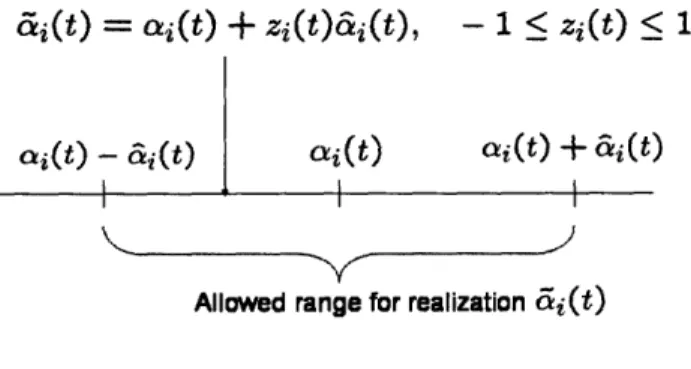
- Pi(t)pi(t) +

where ei(t) is uncertain within a given interval, with unknown probability distribution on that interval. This model essentially assumes an additive demand model, i.e. that there is uncertainty on the demand parameters ai(.), i = 1,...,N. We denote ai(.) the nominal function, &i(.) the realization, and we suppose that the realization belongs to an interval centered around the nominal function with half-length &i(.). This model is illustrated in Figure 2-1.

i(t)

=

ai(t) +

Zi(t)ai(t), - 1 < z(t)

_ 1

Allowed range for realization ii(t)

Figure 2-1: Uncertainty model: illustration for &i(t)

We assume that

0 < &i(.) < oai(.) Vi

and write the constraints as follows:

I&i(t)

- ai(t) < a&i(t)

Vt, i

2.3.2 Budget of uncertainty

To avoid making assumptions that are difficult to satisfy in practice, we do not in-troduce a particular probability distribution on the range described above for the uncertain parameters. However, we do not want to take an overly conservative ap-proach that would allow parameters to be at the value corresponding to the worst-case scenario (typically, one extreme of the allowed interval) at all times, since such a sce-nario is highly unlikely. We favor a more reasonable and realistic approach that would bound from above the cumulative deviation of the realization away from the nominal

;)