Blind estimation of long impulse response and non-minimum phase wavelets application to seismic data

BLIND ESTIMATION OF LONG IMPULSE RESPONSE

APPLICATION TO SEISMIC DATA

AND NON-MINIMUM PHASE WAVELETS

Benayad Nsiri, Thierry Chonavel, Jean-Marc Boucher

ENST de Bretagne, SC Dept, BP 832, 29285 Brest Cedex, FRANCE

email:

Benayad.Nsiri@enst-bretagnefq

Thierry.Chonavel@enst-bretagne.fr

JM. Boucher@ enst-bretagne.fr

ABSTRACT

In seismic deconvolution, blind approches must be consid-

ered in situations where the reflectivity sequence, the source wavelet signal and the noise power level are unknown. In the presence of long, non minimum-phase, source wavelets, strong interference of the reflectors contributions make the wavelet estimation and deconvolution procedure from recor- ded data complicated. In this paper, we address this prob- lem in a two steps approach. First, a robust but truncated estimate of the wavelet is performed using a standard max- imum likelihood approach. Then improved wavelet estima- tion is achieved by fitting an ARMA model to the initial MA wavelet by using the Prony algorithm. The algorithmic problem of wavelet initialization is also addressed. Simula- tion results and real data experiments show the significant improvement brought by this approach.

1. INTRODUCTION

This paper deals with seismic deconvolution, which aims at recovering the geological structure of the underground sed- imentary layers from seismic data records [13]. As usualy

in this kind of situation, the seismic traces are modelled as

the output of a filter that represents the transmitted wavelet, with an input consisting in a two components Gaussian mix- ture: the Gaussian component with high variance models the strong reflectivity at layers interfaces [I]. Recovering

this sequence from the data enables detecting the layers po- sition in the subsurface.

In some experiments of practical interest the wavelet is quite long [13]. In such situations, estimating the model parameters generally yields a high variance of the wavelet estimator. In this paper, we propose a new method that

permits to overcome this problem within the framework of

classical blind seismic deconvolution techniques. More pre- cisely, a two steps approach is proposed the first step yields

a robust Maximum Likelihood (ML) estimate of a truncated

This work was supported by IFREMER

0-7803-7663-3/03/$17.00 0 2 0 0 3 IEEE

version of the wavelet, via a Stochastic Expectation Maxi- mization (SEM) approach. Then, an improved wavelet esti- mation is achieved by fitting an ARMA model to the initial

MA wavelet by means of a Prony algorithm. Furthermore, a

new criterion is also proposed for accurate estimation of the

wavelet impulse response maximum position, which is an

important algorithmic issue for accurate wavelet estimation. The paper is organized as follows: Section 2 describes the

data model, while section 3 is devoted to initial estimation of the parameters. In section 4, improved wavelet estima- tion is considered. Finally, in section 5 we check on simula-

tion and real data experiments the significant improvement brought by this approach. A conclusion is presented in sec- tion 6.

2. DATAMODEL

The observed signal y = ( Y * ) ~ = ~ , N is of the form L

(1)

Yk = h i T k - i

+

W k ,

i=O

where h = (hk)k=o,r. is the wavelet finite impulse response

column vector of length L , r = ( ~ k ) k = ~ , ~ is the reflectiv- ity sequence, and w = ( Z U ~ ) ~ = ~ , N is the observation noise

sequence, with variance ui. The reflectivity process r is

described by a generalized Bernoulli-Gaussian process [I],

characterized by an underlying state model q = ( q k ) k = o , N .

with q k = 1 at high reflectivity points and q k = 0 at low reflectivity points. The corresponding reflectivity rk is dis- tributed according to a zero mean Gaussian distribution with variance u: if q h = 1 or ui if q k = 0,

(2)

p(qk = 1) = 1 - p(qk = 0 ) =

x

T k

-

M(0, U:)

+

(1

-

A)N(O,

U;),

where X is the probability of having a reflector at

a

given position and ut

>>

ug.

3. INITIAL PARAMETER ESTIMATION

We address the blind deconvolution problem through the

classical Maximum Likelihood criterion [3] which leads to

calculate

L v

= a r g m p l n b ( y / o ) ) , (3)

where 8 is the parameter vector of interest. Here, 8 =

In fact, we are faced to an incomplete data problem 13,

61, where the incomplete data are given by z = ( . Z ~ ) ~ = O , N

and Z k = ( q k , T k ) . The joint probability density is ex- pressed by

(h,

A, U,",

d ,

0 ; ) .

p(y,zl8) = P ( Y I ~ , ~ ) P ( Z I ~ ' ) . (4)

P ( Y , ~ I ~ ) = ~ ( ~ l z , ~ ) ~ ( ~ l s , ~ ) ~ ( q l ~ ) . ( 5 ) As z = (9, r), it can also be written

Each component of this equations can be easily expressed.

As q is a vector of independent Bernoulli variables,

N

withp(qkI8) = X q * ( l - A)'-qk. Furthermore, since the T k

are independent, conditional to the variables q k

Then, up to a constant, the complete log-likelihood is ex- pressed by:

L(y, 218) cx-a;*(y - Hr)T(y - Hr) - N.Zn(cr$)

-ul -2 r T

Qr(z)

-

u;'rT(I

-

Q)r(z)

+2qTqzn(U;'X1)

+

2 ( N - qTq)ln(.;'(l

-

A)),

(8)

where Q = diag(q) and H is the convolution matrix asso-

ciated with h. Note that Hr =

Rh, where R is the convo-

lution matrix associated with r. Then, w h y the complete data vector z is known, the derivation of OMV is straight- forward; for fixed (y, z), the ML estimator of 8 is obtained from (8):

6

=

(RTR)-'RTy,

i

= N-'qTq

- r'(r-Q)= 6 2

-

r'

6;

= N-'

11

y -

R6

11:

(9)

6;

N-q'q 1 I-*. where

I/

.

112 represents the quadratic norm.

In practice, z is not known. In such a situation, a SEM (Stochastic Expectation Maximization) algorithm, involv- ing simulation of z, can be used to solve the estimation problem [9]: starting from initial values

do)

and z(') for

0 and z respectively, the SEM

'

it

iteration is of the form

0 SE step: simulate

di)

-

p ( ~ 1 8 ( ~ - ~ ) )

e M step: estimate 8(i) according to eq. (9)

The expression of p(zlO("-')) can be found in 161. In par- ticular, p(rlq,8("-')) is of the form (1 - qk)N(mo,u;)

+

qhN(ml, U : ) . In practice, z can be simulated using a Gihhs

sampler 181. The Gibbs sampler iteration is implemented as

follows [ 6 ] :

For

IC

= 1,.

.

.

,

N ,

Compute p(qk = l l y ; z - k ) , where z-k is z with re- moved k t h entry Z k .

Simulate U

-

Upll

(UE

is the uniform distribution on E ) and take q k = njo,p(q.=lis,.-*)l(") ( E A is the

index function of A ) .

simulate T k

-

(1 - q k ) N ( m O , U ; ) +qkN(ml,u:) 0 update z k : tk = ( q k , T k ) .

let us remark that similar performance results could oh- tained if the above SEM estimation procedure is replaced

by a Markov Chain Monte Carlo (MCMC) approach [14].

4. IMPROVED WAVELET ESTIMATION

In some seismic experiments the wavelet impulse response

h is quite long. In such cases, the mean square error of the

estimator is quite large. In particular, the last coefficients of

h, which have m a i l values, are poorly estimated. For this

reason, searching for a vector h with reduced length gener- ally enables a good compromise between bias and variance properties of the estimator.

However. performing the deconvolution with a truncated

wavelet will generate degradated performance for the retlec- tivity sequence.

Improved ARMA@, q ) wavelet estimation In order to

improve the deconvolution performance, we assume that the MA(L) wavelet model that has been estimated by means

of the SEM procedure described in the previous section is

in fact a truncated version of the true wavelet, of length

L'

>

L. The value of L is not much critical. Simply, the envelope of the MA(L) impulse response should not decay

too much. An efficient approach for choosing L is described

further in the text. Since

L' can

be quite large in prac- tice and, often, the wavelet has an oscilatory shape, it can

be modeled efficiently as an ARMA@, q) impulse response.

In order to estimate it from the initial MA(L) wavelet, we propose to use the Prony method [2]. More precisely, let-

ting h ( z ) represents the transfer function of the ARMA@, q )

model to be estimated, we have

Then, the coefficients

a

= ( a k ) k = l , p and b = (bl)l=o,q are obtained by minimizing the following quadratic criterion:

where we note bi

tions show that (2, b) = argmin,,b J ( a , b) is given by

0 for 1

>

q. Straightforward calcula-

% =

- ( H ~ H ~ ) - ~ H ~ , L

= H,,[I P I T (12) where

Ho =

H1 =

v

=

In order to estimate the respective orders p and q of the

AR and of the MA parts, we use a Kurtosis maximization

criterion [IO].

Initial MA model order selection Now, let us explain how the length

L

of the initial M A ( L ) wavelet can be cho- sen. Denoting hi ( i = 1 1 ,

...,

1 2 ) the estimated wavelet of

length i and

&,,

= (12 - I1 - l)-'

df,,

hi,

we note

M S E i

=I/

hi-h, 112. ComparingMTE =

(M2Ei);=ll,12

and MSE = ( I W S E ~ ) ~ = ~ , , ~ ~ , where M S E i =

116;

- h1)2

(see Figure4). shows that a good choice for L is obtained by

considering the minimum of MTE.

Initialization It is well known that the non-minimum

phase structure of the wavelet h makes its estimation com-

plicated. In particular the wavelet estimation is not robust to initialization. A simulated annealing version of the SAEM

algorithm could he used to overcome this problem [ l l ] . Here, we propose an alternative deterministic procedure for initializing the MA(L) wavelet estimate. As in [ 1 I], we ini-

tialize h with the vector h(2) (i = 1,. . .

,

kl)

that has 0 en- tries, except the i t h one, which is equal to 1, and we perform the deconvolution for each i. Now, let C, = 1 if hi is in- creasing at the origin and C, = -1 if it decreases at the origin. It can be checked that C = ( C i ) i = k l , k z changes of sign at values of i corresponding to the true wavelet lo- cal optima (Figure 3). The retained solution is the one that

maximizes the Kurtosis of estimated reflectivity

i

at such points.

Deconvolution When h bas been estimated, the last step

consists in a deconvolution via an MPM approach that yields

the final estimate of the reflectivity sequence 1141.

5. RESULTS

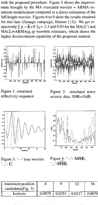
In this section, we present an example for simulated and real data. Figure 1 and 2 represent the simulated reflectiv- ity and observation (U; = l.0-4, X = 0.1,

uf = 0.1). The true wavelet and the function C intro- duced in the previous section are given in Figure 3, while

MSE and MTE are given in Figure 4. Table 1 and Figure

3 show that the maximum position is correctly recovered

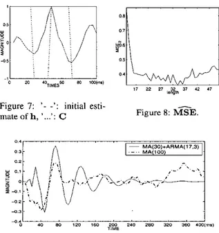
with the proposed procedure. Figure 5 shows the improve-

ment brought by the MA truncated wavelet

+

ARMA ex-

tension modelization compared to a direct estimation of the full length wavelet. Figures 6 to 9 show the results obtained for real data (Zaiango campaign, Ifremer [13]). We get re- spectively

11

y

-

h $

i

/12= 2.3 and 0.93 for the MA(L') and MA(L)+ARMA@, q ) wavelets estimates, which shows the higher deconvolution capability of the proposed method.

=

l l

<(a m m M w m m m

-

OWnE I U P L E

Figure 1 : simulated Figure 2: simulated noisy

reflectivity sequence. seismic data. SNR=IOdB.

figure 3: 3 . .':true wavelet Figure 4: '- -': MSE,

'...':

c.

~...,:MTE.

11

maximum position

11

4

I

9 1 12

/

16

I

candidates(Fig. 3)

U

kurtosis

11

0.0079

1

0.0351

I

0.0217

1

0.0070

Table 1: estimated kurtosis at changes of C

O I 0 3 0 2 3 0 1 0 E g o 41 -0 s 4 3 4 1 0 I 10 l i 20 2 1 Y) S I 10 45 yl SAMPLE

Figure 5: estimated wavelet for SNR=lOdB

0 6 O a t

I

0.d

I/

I

TIMES -0 A -0 6 -0 B A M 800 1 2 M 1501) 2000 2AOO 2800 IBW,mr) Figure 6: registered seismic trace n0602.

Figure 7: ’- -’: initial esti-

mate of h, ’...’: C Figure 8: MXE.

6. CONCLUSION

In this paper, we have proposed a new approach for blind es- timation of long impulse response and non-minimum phase wavelets.

7. REFERENCES

[ I ] J.M.Mende1. ”Maximum-likelihood deconvolution: a journey into model-based signal processing”.

springer-Verlag, 1990.

[Z] Th. Chonavel. ”Statistical signal processing, Mod- elling and estimation”. springer-Verlag, 2002.

[3] AXDempster, N.M.Laird and D.B.Rubin. ”Maxi-

mum likelihood from incomplete data via the EM al-

gorithm”. Joumal of the Royal Statistical Society Ser,vol.B-39:1-38, 1977.

[4] A.E. Gelfand and A.F.M. Smith. ”Sampling-based ap- proaches to calculating marginal densities”. Journal

Amer: Statist. Assoc., 85(410):398409, 1990.

[5] G. Giannakis and J.M. Mendel. ”Identification of non-

minimum phase systems using higher order statistics”.

IEEE Trans. on Acoustic Speech and Signal Process- ing, 37:360-377, 1989.

[6] M. Lavielle. “A stochastic algorithm for parametric

and non-parametric estimation in the case of incom-

plete data”. Signal Processing,voI.42,pp.3-17,1995.

New-York, 1994.

[7] C.P. Robert. ”The bayesian choice”. Springer-Verlag,

[E] S.Geman, D.Geman. ”Statistic relaxation, Gibbs

distribution and the bayesian restoration of im- ages”. IEEE rrans.On Pattem Analysis and Machine

Intelligence,9:721-741,1984.

[9] G.Celeux and J.Diebolt. ”A stochastic approximation type EM algorithm.for the mixture problem”. Stochas-

tics and Stochastics Reports, 22:74?-761, 1989.

[lo] M.Boumahdi. ”Blind identification using the kur-

tosis with applications to field data”. Signal

Processing,48(3):205-216,1996.

[ 111 M. Lavielle and E.Moulines. ”A Simulated Anneal-

ing Version Of the EM Algorithm for non-Gaussian.

deconvolution”. Statistics and Computing,7:229-

236,1997.

[I21 D.Donoho, ”On minimum entropy deconvolution”,

Applied time series analysis 11, Academic Press, 1981,

pp. 565-609.

[I 31 P.Farcy, ”systkme d’acquisition de sismique marine”

ESSR4 campaign Report, DNISESUENSfDTV99-

007,Ifremer. dec. 1999.

[I41 O.Rosec, J.M.Boucher, B.Nsiri, Th.Chonavel, “Blind marine seismic deconvolution using statistical MCMC methods”, submitted to IEEE Oceanic Engineering.