HAL Id: halshs-02878368
https://halshs.archives-ouvertes.fr/halshs-02878368
Preprint submitted on 23 Jun 2020
HAL is a multi-disciplinary open access
archive for the deposit and dissemination of
sci-entific research documents, whether they are
pub-lished or not. The documents may come from
teaching and research institutions in France or
abroad, or from public or private research centers.
L’archive ouverte pluridisciplinaire HAL, est
destinée au dépôt et à la diffusion de documents
scientifiques de niveau recherche, publiés ou non,
émanant des établissements d’enseignement et de
recherche français ou étrangers, des laboratoires
publics ou privés.
Agglomeration Effects in a Developing Economy:
Evidence from Turkey
Cem Özgüzel
To cite this version:
Cem Özgüzel. Agglomeration Effects in a Developing Economy: Evidence from Turkey. 2020.
�halshs-02878368�
WORKING PAPER N° 2020 – 41
Agglomeration Effects in a Developing Economy:
Evidence from Turkey
Cem Özgüzel
JEL Codes: R12, R23, J31.
Keywords: local labor markets, spatial wage disparities, developing country,
Turkey
Agglomeration Effects in a Developing Economy:
Evidence from Turkey
∗
Cem Özgüzel
†OECD
Paris School of Economics
Latest Update: June 11, 2020
Keywords: local labor markets, spatial wage disparities, developing country, Turkey JEL Classification Numbers: R12, R23, J31
∗I thank Güney Celbis, Pierre-Philippe Combes, Hadi Esfahani, Davide Luca, Sandra Poncet, Ariell Reshef and Gregory
Verdugo, seminar participants at University of Paris 1, University of Strasbourg and at the 25th Economic Research Forum (ERF) Conference (Kuwait) for useful feedback. This paper received the Best Paper Award at the 25th ERF Conference (2019). I want to thank the Social Security Institution (SGK) and Turkish Statistical Institute (Turkstat) for kindly providing the data. I acknowledge financial support from the ERF. All errors are mine.
Abstract
Productivity differences across Turkish provinces is one of the highest among the OECD countries. In this paper, I estimate agglomeration effects for Turkish provinces to shed light on the causes of productivity differences and provide evidence on the importance of such effects in a developing country context which literature needs. I use a novel administrative dataset recently made available at NUTS-3 level, for 81 provinces of Turkey for the period 2008-2013 and carry out a two-step estimation. Using a variety of panel data techniques and historical instruments to deal with estimation concerns, I estimate an elasticity of labor productivity with respect to the density of 0.057-0.06, which is higher than in developed countries and around the levels observed in developing countries. I find that domestic market potential matters even more than density and is the most significant determinant of the productivity differences across Turkish provinces. Finally, in stark contrast with the evidence coming from developed countries, I do not find any effects for positive sorting of workers across provinces. This finding suggests that urbanisation patterns may be operating differently in developing countries, indicating the need for further evidence from such countries.
1
Introduction
Despite an extensive literature on the productivity gains associated with large cities in developed economies, little is known about this topic in the developing countries. Investigating agglomeration economies in the rest of the world is necessary for a number of reasons. First, the growth rate of the world’s urban population is being driven by urbanization outside the developed world (OECD, 2020). Given the importance of cities in national economies and the millions of people who live in them, under-standing the drivers of agglomeration economies are policy-relevant for boosting national productivity, reducing regional disparities and improving the well-being of people. Second, one can not assume exist-ing developed world models are applicable to agglomeration economies of the developexist-ing world (Chauvin et al., 2017). For instance, the rapid urbanization observed in developing countries in the second half of the past century stands in stark contrast to the stability seen in the developed world (Glaeser and Henderson, 2017). The rapid growth in urbanization rates, the differences in the growth of cities, insti-tutional or infrastructural qualities may affect the size and the extent of the gains associated with larger and denser cities. In light of these factors, this paper aims to further our understanding of these critical differences by providing evidence from a Turkey, a highly urbanized developing country.
Spatial differences in productivity are driven through three main channels: i) skill composition of workers, ii) local non-human factors, iii) interactions between workers or firms. First, differences in productivity across locations (i.e. cities or regions) could be due to differences in the skill composition of the workers. Workers with higher skills may sort into denser areas if, for instance, skill-intensive industries are not evenly distributed across areas, or if they value cultural amenities more than low-skilled workers. Second, the differences in productivity could be due to local non-human factors. For instance, workers in some locations may have a higher marginal product because of geographical features such as a favourable location (like a port or a bridge on a river), a climate more suited to economic activity, or access to natural resources. Third, local interactions between workers or firms can lead to productivity gains, which is known as Marshallian externalities (see Duranton and Puga (2004) for a review). Thus, to understand spatial differences in productivity, all three channels have to be quantified and considered together.
This paper takes up the challenge of considering all of these factors simultaneously to study the
determinants of wage disparities, a key measure of productivity1, across Turkish provinces.2 Since 1950,
Turkey has experienced urbanization much faster than developed countries due to massive rural-urban migration. Today, 75% of the Turkish population lives in cities, making it a highly urbanized country
1Wages are usually proportional to labor productivity. By using the wages as a measure to compare relative productivity
differences within a country, the literature assumes that the proportion does not vary across regions within the country (Combes and Gobillon, 2015).
2Provinces (il in Turkish), correspond to the NUTS-3 (Nomenclature of Territorial Units for Statistics) level in the
(World Bank).3 In terms of GDP per capita, Turkey has the highest regional disparity among the OECD
countries (OECD, 2018), with substantial spatial inequalities existing across almost every metric (e.g., production or life expectancy). The rapid urbanization experience and significant spatial differences in productivity make Turkey an excellent context for understanding the sources and consequences of agglomeration economies in a highly urbanized developing country.
The analysis uses a novel administrative dataset based on social security records which covers almost the entire universe of workers across all industries, working in both the public and private sector. In addition to its extensive coverage and reliability, the dataset offers the advantage of measuring agglom-eration effects at the province level, a finer geographical unit than any other available data in Turkey. Due to data privacy concerns, the individual observations are aggregated at the industry-province-year level, which makes it impossible to account for spatial sorting of workers based on differences in their observable and unobservable characteristics. I circumvent this problem by complementing my analysis using the Household Labor Force Survey, which provides individual-level data yet at the regional level. Finally, to address endogeneity bias and reverse causality, I use instruments based on past settlement patterns using historical data from the last census from Ottoman Empire and early census of the Turkish Republic.
First, when controlling for local characteristics and addressing reverse causality, I find an elasticity of wages with respect to employment density to be around 0.056-0.06. This means that doubling the employment density in a province increases the average wages (and productivity) of workers by 3.8-4.2%. Compared to other developing countries, this elasticity is lower than those estimated for China (Combes et al., 2015; Chauvin et al., 2017) and India (Chauvin et al., 2017), around those estimated for Brazil (Chauvin et al., 2017) and Colombia (Duranton, 2016), and higher than Ecuador (Matano et al., 2020). Given the levels of urbanization in these countries and Turkey, this elasticity fits precisely where it would be expected, hinting decreasing benefits of agglomeration economies for countries with higher levels of urbanization rates.
Second, I find a positive and strong effect of domestic market potential, on labour productivity. The estimated coefficient is around 0.091-0.1, which is double that of density, suggesting that having access to other markets is the most significant determinant of the productivity differences across Turkish provinces. The estimated elasticity implies that if the market potential of a province doubles, the wages increase by 6.5%. This result corroborates findings from other developing countries which show that productivity gains associated with larger market potential are stronger than developed countries and that they matter for explaining spatial productivity differences (Combes and Gobillon, 2015).
3Turkey went through rapid urbanization starting from the 1950s due to large rural-urban migration. While 34% of the
population lived in cities in 1950, this number increased to 42% in 1975, 53% in 1985, 64.9% in 2000 and it is at 74.5% in 2017 (World Bank). Most of the internal migrants were low-skilled agricultural workers (Kirdar and Saracoglu, 2008). While 62.5% of the Turkish labor force was employed in agriculture in 1980, only 18% remained in this sector as of 2018 (Turkstat).
Third, I do not find any effects of sorting of workers across locations according to their observable skills. This result is in sharp contrast with what is usually observed for developed countries, where a large fraction of the explanatory power of city effects arises from the sorting of workers (Combes and Gobillon, 2015). It is, however, very much in line with the results for China (Combes et al., 2015, 2020), which suggests that urbanization patterns may be operating differently in developing countries, supporting the need for further evidence from such countries (Chauvin et al., 2017).
Finally, I find a weak relationship between productivity (wages) and amenities. This result echoes the findings in other developing countries and can be explained by either the high correlation between density and amenities (Duranton, 2016); or that workers in developing countries are not rich enough to forgo part of their income to live in areas with better amenities (Chauvin et al., 2017).
This paper makes several important contributions. First, the paper is the first to estimate agglom-eration economies in Turkey and consider a broad set of factors that influence productivity differences simultaneously in a developing country context. Considering a broad set of explanatory factors allows quantifying the magnitudes associated with each explanation and comparing their relative importance. Given the importance of productivity as a driver of growth, understanding which local factors make a given worker more productive is crucial for formulating policies to reduce regional disparities. Second, estimated magnitudes for local characteristics such as density or domestic market potential indicate stronger effects compared to those observed in developed countries. These results further our under-standing of the importance of local characteristics given the urbanization rate of a country. Third, the absence of positive sorting effects and a weak relationship between wages and amenities highlights a fundamental difference between developed and developing countries regarding the drivers of urbaniza-tion. These findings corroborate recent evidence from developing countries that show that while the main mechanisms of urban economies are present in the developing world, the current models need to be extended to capture the differences observed in the developing part of the world which has experienced fast urbanization rates.
The rest of the paper is organized as follows. Next section provides details about the Turkish context (Section 2), followed by Section 3 which presents the data used in the analysis. Section 4 presents the empirical strategy and discuss the identification issues. Section 5 provides estimates on density and other determinants of productivity. Section 6 concludes the paper.
2
The Turkish context
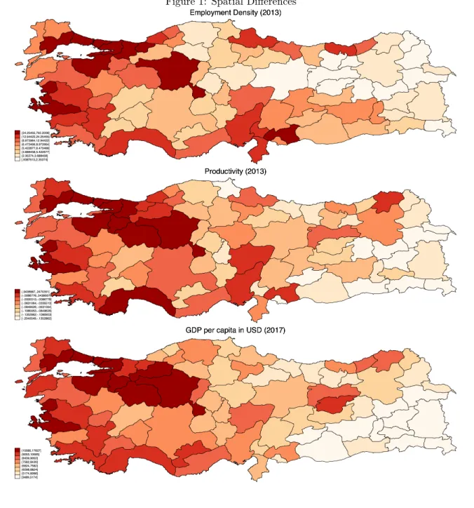
Turkey has a population of about 81 million people over an area of 783 thousand square kilometres (Turkstat, 2019). With a Gross Domestic Product (GDP) per capita of USD 10546 in 2017, according to the World Bank Turkey is an upper-middle-income developing country. However, this wealth is not
equally distributed across its regions (See Figure 1). While the GDP per capita in Istanbul was USD
17827, it was only USD 3489 in Ağrı (Turkstat, 2019).4 These differences are multiplied even further
at the aggragate level since population distribution is also uneven. In 2017, while 18.6% (15.1 million people) lived in Istanbul province, 6.7% (5.4 million) and 5.2% (4.3 million) lived in Ankara and Izmir, respectively. The population density of Istanbul, the densest province, is 2892 persons per square km, while it is only 11, in the least dense, Tunceli (Turkstat, 2019). All in all, while Istanbul is producing 31.5% of the national GDP, adding its immediate surrounding area increases the share to 39% in 2017
which creates large imbalances across regions in terms of production and income (Turkstat, 2019).5
[Figure 1 about here.]
2.1
Literature on regional differences in Turkey
Turkish regional imbalances has been the focus of a number of papers over the years. While some papers used provincial income data to study the spatial income inequalities (Atalik, 1990; Gezici and Hewings, 2004; Luca, 2016), others focused on provincial and regional convergence of income (Kirdar and Saracoglu, 2008; Celbis and de Crombrugghe, 2018).
Although there has been considerable number of studies dealing with the determinants of overall productivity at the national level (Altug et al., 2008; Ismihan and Metin-Ozcan, 2009; Atesagaoglu et al., 2017) or in the manufacturing sector (Krueger and Tuncer, 1982; Onder et al., 2003; Atiyas and Bakis, 2014), regional level analysis has been limited. Few examples include Metin et al. (2005) who study TFP growth in the Turkish manufacturing industry in eighteen provinces from 1990 to 1998 or Temel et al. (1999) who use gross provincial product per worker for the period 1975-1990. These papers find evidence of concentration of high productivity activities in a few highly industrialized regions while most provinces tended to move towards low productivity activities, creating regional divergence in terms of productivity.
Determinants of spatial productivity in Turkey has not been addressed in the literature. Coulibaly et al. (2007) is the closest work in spirit, to this paper. The authors assess the impact of urbanization on sectoral productivity between 1980 and 2000 by using manufacturing data and geographical, infras-tructural and socio-economic data at the province level. Their results suggest that localization (similar to specialisation which measures how much local production is concentrated in a given activity) and urbanization economies, as well as market accessibility increase productivity. Authors do not, however, deal with identification issues such as endogeneity of local determinants of agglomeration economies or the sorting of workers.
This paper is the first causal evidence from Turkey focusing on the spatial productivity differences
4Regional imbalances in Turkey go back to late Ottoman Empire. For more details on the historical background of
geographical disparities see Appendix Section A.
through agglomeration literature perspective. The novel data that I use in this paper (see the next section), also makes it the first paper that analysis productivity differences at province level covering the period after 2000.
3
Data and Sample
The paper uses different data sources to estimate the determinants of spatial differences in wages. This section presents the main data used in the analysis.
3.1
Data
3.1.1 Social Security Data
In this paper, I use a novel administrative data set that was made available to researchers recently. This data set is collected by the Social Security Institution (Türkiye Cumhuriyeti Sosyal Güvenlik Kurumu -SGK) and are based on administrative records for all the workers affiliated to the social security system.
It covers employment in all of the industries, in the private and public sector.6
Due to data privacy issues, the raw individual-level data is aggregated by the SGK by sector, province and year. Thus the data includes yearly information on the number of workers, the total number of days worked, the number of firms and total payments received (wages and benefits) by the workers, for 81 provinces, grouped according to Nace Revision 2 at 4-digit sector level (659 sectors) from 2008 to 2013. The data is further disaggregated by job contract-type (temporary vs permanent), by sex (male vs female) and legal status (public vs private-owned).
The novelty of this data is that it makes analysis at province-level possible. The literature focusing on individual or firm-level outcomes has been limited to analysis at region level (NUTS-2) due to data
availability.7 This dataset makes it possible, for the first time for the period since 2000, to focus on
productivity differences at a geographically more disaggregated level. This is also the first paper to use this dataset.
The final sample for analysis includes male and female workers employed in private sector8, holding
temporary and permanent job contracts in Turkey from 2008 through 2013. This amounts to 168 904 industry-province-year observations, which I use to estimate the province-year fixed-effects in the first step.
6The data covers all employment with compulsory insurance in the private and public sector under Article 4-1/a and
4-1/c of Act 551. For the year 2013, this corresponds to 13,1 million formal employees in private (12,5 million) and in public (650 thousand) sector. It does not include apprentices (321 thousand), those who work abroad but are affiliated with the Turkish Social Security System (35 thousand), the agricultural sector (64 thousand) and voluntary based insured partially employment (230 thousand). It does not include the self-employed (2.9 million) who are covered under Article 4-1/b of Act 5510.
7Two main data sources used in studies focusing on the Turkish labor market are Household Labor Force Survey
(Hanehalkı İşgücü Anketi ) and Annual Industry and Service Statistics (Yıllık Sanayi ve Hizmet İstatistikleri ) which are provided by Turkish Statistical Institute (Türkiye İstatistik Kurumu). Both datasets allow identification at NUTS-2 level.
3.1.2 Household Labor Force Survey
I complement the main analysis by using individual level data obtained from the Household Labor Force Survey (Hanehalkı İşgücü Anketi, in Turkish, LFS henceforth) prepared by the Turkish Statistical Institute (Türkiye İstatistik Kurumu, in Turkish, Turkstat henceforth). The LFS is representative of the total population in Turkey and is used to follow the state of the economy and the labor market, both at the regional and national level. The LFS includes annual information on economic activity, occupation, employment status, hours worked (for persons employed in formal or informal sector), unemployment, education and more.
In the period of my analysis, each survey wave included around 135 thousand households, covering 500 thousand individuals. Its high level of detail and large sampling size makes it an important data source for research on the regional and national labor markets in Turkey (e.g., Tumen, 2016; Balkan and Tumen, 2016; Baslevent and Onaran, 2003, 2004).
The main shortcoming of this dataset is that it allows analysis only at regional level (NUTS-2). In my analysis, I prefer using the social security data, which will enable me to study the local interactions at a lower geographical unit (i.e., province-level, NUTS-3) and use the LFS as a complement to address identification issues.
3.1.3 Historical Data
Since Ciccone and Hall (1996), it is standard practice to use long-lagged variables as instruments for local characteristics. Following the literature, I construct various instruments using Ottoman Empire population statistics of 1914 and the Turkish Republic’s population censuses of 1927, 1935 and 1945. The last Ottoman census was conducted in 1905/1906 and population statistics of 1914 is an updated version of this census. The 1914 population data used in this study were published for the first time by
Karpat (1985), adapted to current administrative borders by Sakalli (2019).9 I complement this data
by digitizing published census reports for the period 1927, 1935 and 1945 which come from Turkstat. In addition to the population statistics, these data also include information on occupations, number of students, number of schools and much more.
I use these data to calculate the past population densities and past domestic market potential. I also use the number of enrolled male students to elementary schools and high schools in 1927. Finally I compute the foreign-market potential using historical GDP data for Turkey’s trading partners coming from the Maddison Project Database (Bolt and van Zanden, 2014).
9Between 1914 and 2007, the number of districts, names, and their borders has changed considerably. I use the
4
Empirical Strategy
This section presents the framework used for estimating the agglomeration effects in Turkey. It also discusses possible identification issues arising from reverse causality and selection bias due to sorting of workers by their ability.
4.1
Econometric Equation
To evaluate the impact of agglomeration economies on productivity, I use a two-step estimation strategy that is standard in the literature:
logwpst= α + δlogSpepst+ γs+ γpt+ εpst (1)
γpt= ν + β1logDenpt+ θXpt+ φZp+ γt+ εpt (2)
In the first step (Equation 1), I regress the log average daily wages (logwpst) in province p, sector
s at time t,10 on logSpepst which captures the effect of specialisation in a given sector on productivity.
The panel structure of the data (81 provinces, 659 industries and 6 years), allows me to introduce sector
fixed-effects (γs) which capture sector-specific differences in the productivity that is irrespective of time
(e.g., average labor productivity is higher in manufacturing sectors than in agriculture ). Province-year
fixed effects (γpt) can be considered as local wage indices after controlling for industry fixed-effects and
localisation economies. Finaly εpstis the error term representing unexplained productivity net of controls
and fixed-effects.
The province-year fixed-effects estimated in the first step are then used as the dependent variable in the second step (Equation 2) and regressed on local characteristics that impact the productivity levels.
To account for the local structure I use density (logDenpt), where Denptis the total number of employees
(or population11) in province p at time t (emppt) divided by land area (Areap).12
The estimation of density could suffer from omitted variable bias. To address this concern, Xpt
includes time-varying controls from economic geography literature (e.g. market potentials, diversity,
10I calculate the daily wage by dividing the average monthly salary by the number of days worked.
11Depending on the mechanism studied, agglomeration effects can be measured using employment, population, or
pro-duction. Since these three variables are highly correlated separate identification of their impact is not possible. I use employment (instead of the population) as it reflects better the magnitude of the local economic activity (Combes and Go-billon (2015)). Moreover, given that some of the local variables (such as diversity or specialisation) can only be constructed using employment data, it is more consistent to measure the employment density.
12Since Ciccone and Hall (1996), it is customary to measure the size of the local economy using density, which is the
number of workers (or individuals) per unit of surface area. Although the number of employees can also be used directly, dividing over the land area is preferable as it addresses concerns due to heterogeneity in the spatial extent of the geographic units that are used. Moreover, the use of density adresses the concerns about the shape of the unit of analysis (due to the arbitrary administrative borders) which is known as the modifiable areal unit problem in the literature (Briant et al. (2010)). The β captures the total impact of local characteristics related to agglomeration economies rather than the magnitude of specific channels through which agglomeration forces operate. Moreover, it is the total of the net effects of density, which could be both positive due to agglomeration economies but also negative due to congestion costs.
human capital, road network, and more.) while Zp, includes the time-invariant controls (e.g., land
area, temperatures, geographic controls, etc.). Beyond their importance for identification of an unbiased estimate, their inclusion also makes it possible to quantify relative importance of each determinant in the overall productivity. Appendix Section B details the importance of these variables, their construction
and data sources for each variable. γtis the year-fixed effect, which absorbs any temporal variations that
affect the productivity of all provinces and sectors equally (e.g. productivity gains from technological progress). The use of time fixed-effects also addresses concerns due to the use of wages in current Turkish
Lira and is more precise than using an arbitrary price deflator (Combes and Gobillon, 2015). 13
This method is preferable for two reasons. First, doing a two-step estimation allows for estimating
two separate error terms one for province-sector-year (εpst) and one for province-year (εst). This makes
it possible, in a second-step, to tackle the endogeneity of density and other location characteristics
without addressing the sector-specific endogeneity issues, such as specialisation (logSpepst). Second, this
procedure makes it possible to sepearately identify the localization economies (first-step) from those that are due to urbanization (second-step) as well. This is particularly important for policy formulation as it helps determine whether policy focus should be on further developing existing sectors or encouraging
the arrival of new activities to the region.14
4.2
Estimation Issues
There are two sources of bias in the estimation of the equation above. First, workers may prefer to locate in large cities where wages are higher, creating a reverse causality problem between density and wages. Secondly, workers with higher ability may sort to larger cities which can bias positively the estimated elasticities. This section details these estimation issues and explains how I deal with each one.
4.2.1 Estimation Issue 1: Circular Causality
First identification issue is due to possible simultaneity between local characteristics and local wages. For example, employment areas receiving a positive technology shock may attract migrants, which would, in turn, increase the density of employment and further increase the wages. Such factors can generate
13Nominal wages are a better of measure for capturing differences in the productivity compared to real wages, which would
be capturing differences in “standard of living” (Duranton, 2016). The estimation of local real wages requires considering the cost of living, specifically land prices. Given that such data is rarely available, nominal wages are used to have a consistent measure of productivity.
14The estimation can be done in a single-step. However, this estimation would be problematic because it does not allow
computing the variance of local shocks. This makes it impossible to distinguish local shocks from purely idiosyncratic shocks at the industry-location level, which is vital with missing endowment variables. Furthermore, in a single-step estimation, the variance of local shocks has to be ignored when computing the covariance matrix of estimators. This can create significant biases in the standard errors for the estimated coefficients of aggregate explanatory variables (Moulton, 1990). To address this problem Combes et al. (2008) propose a two-step estimation strategy which both solves this issue and has the advantage of corresponding to a more general framework. As a robustness check, I run a single-step estimation and find very similar results. Results can be provided if requested.
a positive correlation between employment density and wages, causing an upward bias in the estimates. Other regressors such as market potential or human capital are also likely to be endogenous since they also depend on workers’ and firms’ location decisions.
Several instrumentation strategies have been proposed in the literature to address this endogeneity issue (Combes and Gobillon, 2015). Using historical instruments, as proposed by Ciccone and Hall (1996), is the most popular method and it builds on the hypothesis that historical values of population (or density) are relevant for today’s levels as they are persistent over very long periods. The local outcomes of today (such as productivity or types of economic activities), however, are unlikely to be related to the economic outcomes a long time ago that probably affected the historical population. Following this strategy, I construct various instruments using Ottoman Empire population statistics of 1914 and the Turkish Republic’s population census of 1927 and 1935.
Using these historical population numbers, I build variables that capture population densities and growth. The instruments are valid in the case of Turkey for a few reasons. First, it is unlikely that density levels from almost 100 years ago to be correlated with labor productivity today, as the Turkish economy went through a wide range of productivity shocks during this period. Successive wars between 1914 and 1923 had a significant impact on physical and human capital stock while disrupting industrial and agricultural production in most parts of the country (Pamuk, 2014). In addition, considerable population shifts took place between 1914 and 1924, which caused a dramatic reduction in the share of employment in the non-agricultural sector. The urban population was disproportionately affected by the decade-long wars and in their aftermath (Altug et al., 2008).
Economic government and policies have seen important changes as well. Following the transition from a multi-ethnic, multi-religious empire to a nation-state under a democratic and representation rule, the newly founded capital Ankara created policies that presented a contrast to the past. As discussed in Appendix Section A, Turkey went through important sectoral re-allocation and experienced a significant structural transformation. Massive public investment in human capital increased literacy rates from around 10% in 1923 to 90% in 2007 (Altug et al., 2008), while urban population increased dramatically following the large-scale mechanization in 1950s which freed up labor in rural areas.
I construct past domestic market potential using 1935 and 1945 population numbers, and past foreign market potential using the GDP levels of the main trading partners of Turkey in 1945 using the Maddison Project Database. In the main specification, I jointly use several instruments (instead of using only the 1914 urban population) for two reasons. First, having multiple instruments allows me to the instrument not only for employment density but also for the market potential, diversity, and even land area. Second, it makes it possible to carry out over-identification tests. Although I use multiple instruments in the main estimations, I also provide robustness tests using various single instruments.
character-istics can be argued for almost all of them, I choose to instrument at most three of them simultaneously, as more than that would be extremely demanding in terms of identification power. I estimate these instrumented regressions either controlling for all or none of the non-instrumented variables and show
that the results are consistent in both cases.15
4.2.2 Estimation Issue 2: Sorting by ability
The second identification problem is the possible correlation between density and worker characteristics. If workers’ spatial distribution depends on their abilities, then the local productivity would also be affected by the differences in the composition of workers. In the case of sorting based on ability, the estimated impact of local variables would be inflated as they would be capturing productivity gains that are also due to differences in the composition of the workers’ abilities that are observed and unobserved. The sorting of more-skilled workers into larger cities is observed in the US and Europe (Combes et al. 2008; Baum-Snow and Pavan 2012; De la Roca and Puga 2017). In the case of the US, Baum-Snow and Pavan (2012) find sorting based on observables characteristics, yet none due to unobservable ones. In the case of France, however, Combes et al. (2008) show that controlling for observable skills is not enough to remove the bias. Contrasting the evidence from these developed countries, Combes et al., 2015 and Combes et al. (2020) find very weak sorting effects based on observables in China. This weak relationship makes them conclude that in the absence of sorting based on observables, sorting due to unobservable characteristics is unlikely. These results show that both the degree of bias and its direct channel (i.e., observable or/and unobservable) are specific to each context.
The most commonly used strategy is to use a panel of workers and estimate the parameter by comparing the same workers across several locations as suggested by Combes et al. (2008). However, such data is hard to find in developing countries. An alternative solution is to control for an extensive set of individual characterists to take care of differences in the observable skills (Duranton 2016; Chauvin et al. 2017; Combes et al. 2020). If workers, howewer, sort across locations based on their unobservable abilities, this method is not enough to fully address the potential bias.
If such bias exists in Turkey, then a positive correlation between average wages and city charac-teristics could reflect a composition effect due to the over-representation of more able workers in some provinces. The inclusion of human capital as a control addresses concerns due to sorting based on ob-servable characteristics. The sorting based on unobob-servables, however, would not be possible to address when using data aggregated at industry-province level. It is thus important to see whether such sorting exists in Turkey and if so, measure its size. To measure the potential bias due to sorting, I use the House-hold Labor Survey and exploit its individual-level dimension to account for sorting based on observable characteristics.
5
Results
In this section, I start by estimating the elasticity of wages to density by addressing gradually each iden-tification concern discussed previously (Section 5.1). Then I present results of a multivariate framework accounting for local characteristics that determine the local productivity (Section 5.2). I end the section with estimations that include infrastructure and other amenities (Section 5.3).
5.1
Density
I apply the two-step regression methodology where in the first-step I estimate province fixed-effects which
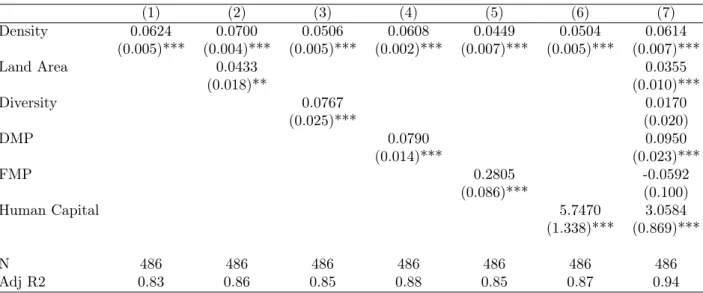
are used as the dependent variable in the second step.16 Table 1 presents OLS results for the second step
of the estimation. Each column corresponds to a different model using observations over 6 years for 81 provinces. I use weights that are proportional to the number of observations used to compute the LHS variable as it corrects for heteroskedastic error terms and thereby achieve a more precise estimation of
the coefficients (Solon et al. (2015))17. Standard errors are clustered at province-level.
[Table 1 about here.]
Column 1 of Table 1 shows that density has an elasticity of 0.06. This means that in the cross-section of Turkish provinces between 2008 and 2013, doubling the worker density increases the average
productivity by 4%.18 Concretely, if density of Iğdır (2.96, P25) were to increase to density of Mersin
(11.3, P75), its productivity would increase by 14.7%.19
In the following columns, I address the omitted variable bias by adding a number of controls that are
standard in the literature.20 In Column 2, I add the land (surface) area of the province. The impact of
land area is significant, which is in line with the literature. The positive coefficient suggests that, holding density constant, a 1% increase in the land area, increases the average productivity by 0.04%. The elasticity of density (β = 0.06) increases slightly compared to Column 1, although given the standard errors, I cannot reject the null hypothesis that they are equal. In Column 3, I add diversity control, which is also very significant. The elasticity of density drops to 0.051, suggesting that provinces with higher employment density also have a more diverse industry structure. In Column 4 and 5, I separately add controls to capture the domestic market potential (DMP) and the foreign market potential (FMP). Both controls are highly significant, and they reduce the elasticity of density.
16Although the first-stage is not reported, all of the estimated province fixed-effects and specialisation are highly
signifi-cant (p<0.001). The estimated elasticity of log of specialisation is 0.065. This means that 1% increase in the specialisation of the local industry increases the average wages by 0.065%.
17All of the results reported in the paper carry through without weights. 1820.06− 1 ≈ 4%
19This elasticity is the result of pooling observations across 6 years. However, as can be seen in Appendix Table D1, the
coefficient remains stable when the regression is repeated separately by year. The yearly results also address any concerns related to pooling of 6 years of observations together and instrumenting with time-invariant historical variables. As can be seen from the results, coefficients remain highly stable and statistically significant, while the standard errors are small.
20It is important to note by including these controls, I make the implicit assumption that the controls are exogenous.
Furthermore, these regressions ignore the endogeneity concerns due to reverse causality and individual unobserved hetero-geneity. I address both concerns in the following sections separately.
In Column 6, I account for human capital by adding the share of the population with a university degree or higher. The control is highly significant, and its inclusion reduces the coefficient of density which is expected given the high correlation between density and human capital levels. This implies that about 20% of the relationship between wages and employment density is explained by worker characteristics and (possible) human capital spillovers. It is important to note, however, that human capital control is a share and is a semi-elasticity.
Finally, in Column 7, I include all of the controls to provide estimates that are comparable to the literature. When all controls are included, the coefficient of density is 0.0614 and is highly significant. This means that doubling the density of a location increases the average productivity by 4%, when all else is equal. While the land area remains significant, diversity turns insignificant which is in line with the literature (Combes and Gobillon, 2015). When regressed along with the domestic market potential, the foreign market potential becomes insignificant. This common problem is due to the high correlation between the two variables (≈ 0.93) and the lack of spatial variability of the foreign market demand
given the way the variable is constructed.21 That is why, in the following sections, I work only with the
domestic market potential. Lastly, the contribution of human capital remains powerful and significant.
5.1.1 Reverse Causality
The second important estimation issue is the reverse causality between density and wages. I address this concern and the potential bias it generates by implementing an IV strategy. This exercise is essential for the estimation of an unbiased elasticity because a good instrument would take care of both the reverse causality and the omitted variable bias addressing both concerns simultaneously.
My main identification strategy consists in implementing the 2-stage-least-squares (2SLS) estimation outlined in Section 4. I use the estimated province-year fixed-effects as dependent variable and include only density as an explanatory variable. In order to address the endogeneity of the main variables of interest, I use various historical instruments that are based on historical census data from 1914, 1927, 1935
and 1945. Seperately, I instrument logDenpt with population density in 1914 (logDenp1914), population
density in 1927 (logDenp1927), employment density in 1935 (logDenp1935), employment density in 1945
(logDenp1945), and growth in population density between 1914 and 1927 (DenGrowthp).
Figure 2 provides a visual representation of the first stage for density. It plots the density in 1914 in the horizontal axis against the average density in 2008 and 2013. Each observation in the figure corresponds to a province.
[Figure 2 about here.]
The figure shows that density in 1914 is a good predictor of the density today. I formally test the validity of each instrument by reporting the first-stage regression using the following equation:
logDenpt= ν + θ1logDenp1914+ γt+ εpt
Table 2 reports the coefficients from the first-stage regression. The coefficient θ, reported in the table represents the effect of the past densities on the current density levels. In line with the main specification, all of the regressions include time fixed-effects and errors are clustered at the province level.
[Table 2 about here.]
Each column presents the coefficients from regressions where I use a different instrument. In the first column of Table 2, I use the population density in 1914. The estimated coefficient is highly significant and around 1.17 which is similar to estimates reported in Combes et al. (2011). Specifically, an increase in the imputed past density by one percentage point leads to a 1.17 percentage point increase in the worker density between 2008 and 2013.
In the following columns, I repeat the exercise using densities from more recent years. All of the instruments regardless of the base year used or whether they capture employment or population density,
pass the weak instrument test.22 As expected the F-statistic gets larger when I use densities from more
recent periods. Results show that population densities at the beginning of the 20th century are good predicter for the employment density in 2008 and 2013 period due to the strong inertia of the urban hierarchy in Turkey. However, given the significant changes that took place between two periods, it is unlikely that they are correlated to labor productivity.
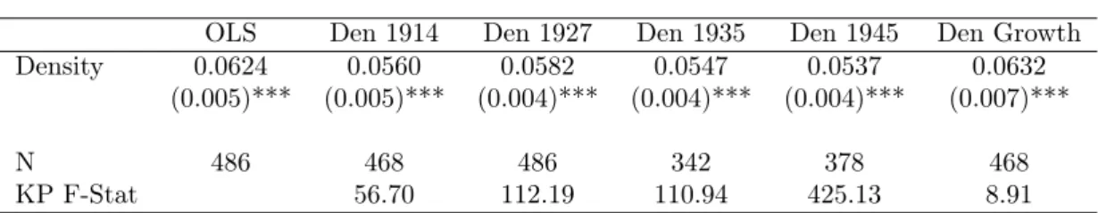
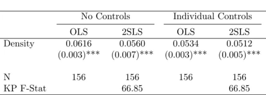
Table 3 presents the results for the estimation of Equation 2.23 As explained previously, the parameter
β1 corresponds to the effect of employment density on the productivity levels of the provinces.
[Table 3 about here.]
In the first column, I report the elasticity obtained through OLS estimation. In the following columns, I present 2SLS results where the density is instrumented with lagged densities that are reported in the header of each column. In the final column, I use the change in the population density between 1914 and 1927 as an additional instrument.
Few results stand out. First, regardless of the instrument, the elasticities remain stable and highly significant around 0.056-0.06. This suggests that the OLS estimates suffer from a positive bias around 10%, which is in line with the literature (Combes and Gobillon, 2015). Second, all of the instruments have strong first-stages, proving to be good predictors. It also shows that the results are not dependent on the use of a specific instrument and are thus robust. Third, the standard errors are very small, indicating high precision of the estimates. Finally, the elasticities are very similar to that found in the
22The number of observations in Columns 4 and 5 is lower due to differences in the number of provinces. Between 1923
and 2008, the number of provinces went from 57 to 81. The historical data in 1914 and 1927 were at district level, which allowed me to combine them according to the province boundaries in 2008. The data for 1935 and 1945, however, were only available at province-level. This made it impossible to distribute them according to the current number of provinces.
final column of Table 1 indicating that valid instruments can take care of both the bias due to reverse causality and missing variables.
Table 3 shows that once instrumented elasticity of productivity to density is between 0.056-0.06. This means that doubling the worker density increases the average productivity by 3.8 - 4%. This elasticity is comparable to those found in other countries that use similar specifications with aggregate data. It is similar to 0.06 found in Combes et al. (2008) for French employment areas over the period 1976-1998, 0.05 in Ciccone (2002) for the five largest EU-15 countries at the end of the 1980s, 0.06 found in Ciccone and Hall (1996) for American counties in 1988. These numbers are much higher than the estimates using individual level data and individual fixed effects, which find elasticities between 0.01 and 0.03 (Combes et al., 2008; Ahrend et al., 2017; De la Roca and Puga, 2017).
Compared to estimates in other developing countries, the elasticity of density is higher than 0.035 found in Ecuador (Matano et al., 2020) or 0.05 found in Colombia (Duranton, 2016), but lower than 0.09–0.12 found for India (Chauvin et al., 2017) or 0.10-0.12 found for China (Combes et al., 2015).
Given the level of urbanization in Turkey, this elasticity fits precisely where it would be expected.24
5.1.2 Sorting By Ability
If workers sort across locations based on their observed and unobserved abilities, the estimates can be biased up to 100% as shown in Combes et al. (2008) in the context of France. However, it is also possible for the bias not to exist if there is no correlation between individual characteristics (observed and unobserved) and local characteristics as found in China (?Combes et al., 2017). This section explores whether sorting exists in Turkey and, if so, measure its importance.
Given that SGK data lacks the individual complement, it is impossible to test the existence of such bias and net out its effect if it exists. As a way to detect the presence of such bias, I use Household Labor Force Survey (LFS). The survey is conducted every quarter to measure the state of the economy. It covers around 500 000 individual observations annually, including all ages and both genders. It is sampled to be reflective of the Turkish population but also of the state of the economy, as it is used for calculating unemployment rate and other labor market measures.
The main shortcoming of this data, given the objective of this paper, is that it is aggreagated at NUTS-2 region level. This means that the locations of individuals can be identified only at one of the 26 regions which is a shortcoming as smaller geographical units are better for capturing benefits of
interactions that decay with distance (Combes and Gobillon, 2015).25 Still, using larger local units may
24Due to absence of panel data in the developing countries, these papers use individual-level cross-sectional data, which
allows them to net out the endogeneity bias due to only the sorting effects based on observable characteristics. Thus their elasticities present gains that are due to agglomeration economies generated by the higher densities (and possible sorting effects based on unobservables).
2526 regions correspond to the NUTS-2 level. These regions have different geographical and population sizes. NUTS-2
regions such as Istanbul (TR10), Izmir (TR31) and Ankara (TR51) are identical to the NUTS-3 provincial borders. Other regions are formed by combining multiple provinces. See Appendix for a map.
not be an important issue. According to Briant et al. (2010) using consistent empirical strategies (i.e. accounting for individual selection) largely reduces issues related to shape and size of the unit of analysis, and allow the estimation of unbiased estimates.
Different waves of the LFS are repeated cross-sections with no individual identifiers which makes it impossible to use individiual fixed-effects. To examine the existence of a possible selection, I carry out two tests following follow Combes et al., 2015 and Combes et al. (2020).
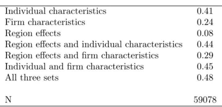
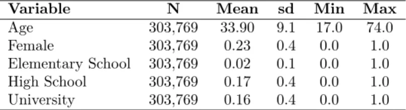
As a first test, I examine the sources of spatial variations in wages. I begin by estimating the first step estimation including different sets of explanatory variables (location effects, individual characteristics, and firm characteristics) to understand their relative contribution to the log of the monthly wage. Table
4 reports the adjusted R2 of each regression using observations from 2009.26
Individual characteristics (i.e., education, age, and sex) alone explain 41% of the variations in indi-vidual wages. The explanatory power of firm characteristics (i.e., firm size) is 24%. Region effects (i.e., region dummies and specialisation) explain only 8%. These results suggest that individual characteristics are the main factors explaining individual wage disparities, followed by firm effects. The location effects and specialisation matter very little.
[Table 4 about here.]
These results reveal that three sets of effects are fairly orthogonal. Region effects and individual
characteristics together explain 44% of the wage disparities while the sum of their individual R2is 0.49.
Similarly, while region and firm effects explain 29% of the variation, the sum of their individual R2 is
0.32. Finally, individual and firm characteristics explain only 45% of the differences in wages, the sum of
their individual R2 is equal to 0.65. These results suggest that differences in observed wages cannot be
attributed to differences in the composition of the labor force or the type of firms present. The absence of correlation between the effect of individual characteristics and region dummies suggest that workers do not sort across regions according to their observable characteristics.
To further examine the absence of sorting in Turkey, I carry out a second exercise. If individuals sort across regions according to their abilities, some local variables, especially the density, should be correlated with individual observables such as education or occupation. It is possible to test this by estimating the region-year fixed-effects with and without individual characteristics in the first step of
the estimation.27 If workers sort across locations by their observable characteristics, these estimated
fixed-effects should absorb them, and thus provide different results in the second step.
I combine multiple waves of the Household Labor Force survey for the period 2008 and 2013, and
create a sample that matches the SGK data.28 This leaves me with 412 137 individual observations over
26Full estimation results are available if requested. 27See Appendix Table E1 for the results.
28Similar to the SGK sample, I keep all male and female workers, who are between 18-65 years of age, with positive
the 6 year period which I use in a two-step procedure with individual level data similar to Combes et al. (2008). The procedure consists in estimating the following specification:
logwirst= α + δlogSperst+ φZit+ γs+ γrt+ εirst (3)
γrt = ν + β1logDenrt+ γt+ εrt (4)
The first step estimation of equation 3 evaluates the impact of individual i’s wage at year t, wirst, of
region-time fixed-effects, γrt, for region r where worker i is employed at year t and region r’s specialisation
in sector s where i is employed (for 88 Nace 2 industries), and a set of individual characteristics Zit,
such as age, age squared, sex, education (7 groups), occupation (39 ISCO 88 categories). In the second
step, I use the estimated region-year fixed effect, γrt, as the dependent variable and regress it on region’s
employment density (logDenrt) and time fixed-effects, γt.29
[Table 5 about here.]
Table 5 reports OLS and 2SLS results for the second step.30 In Columns 1 and 2, I regress the
region-year fixed-effects which are estimated in the first step which includes only region-year dummies and specialisation control. In Columns 3 and 4, I regress region-year fixed-effects, which are estimated in the first step where I include also a set of individual characteristics. While the first-step is weighted with survey weights, the second-step is weighted with the number of workers used to estimate the region year fixed-effects in the first-step. All regressions include year fixed-effects and errors are clustered at the region-level. In Columns 2 and 4, I instrument the current employment densities with the population density in 1914.
The elasticity of density remains stable across specifications, regardless of whether individual controls are included or not in the first step. Although inclusion of individual controls improves the precision of
condition. First, I drop workers in the informal sector to match it with SGK data in terms of coverage. Second most of the evidence in the literature use data in the formal sector (e.g., Combes et al., 2008; D’Costa and Overman, 2014; De la Roca and Puga, 2017). By focusing on formal employment allows me to provide numbers that are comparable with the literature. Still, in Appendix Section G, I provide estimates including also workers in the informal sector. I drop self-employed as it could mean a large set of occupations (e.g., street vendors, shop owners) in a context like Turkey and are also not included in the SGK data. Although not reported, I also tested the robustness of the results to make sure that they are not dependant on the sample selection. Inclusion of public sector employees slightly reduces the elasticity of density to 0.047-0.053, while the inclusion of self-employed does not change elasticities. Results are available if requested.
29I measure density using the survey data for consistency. In Appendix Table E1, I test the robustness of my estimate
by measuring employment density using the SGK employment data. Results are almost identical.
30First-stage results are presented in the Appendix Section E.1. All the variables have the expected signs and are
statistically significant. One result that is worth pointing is that the estimated elasticity of (log) specialisation is much smaller (0.0279) than the elasticities found in the main results using data aggregated at industry-location-year (0.06). The individual-level LFS data allow accounting for the individual characteristics (e.g. education, occupation) and estimating the effect of specialisation net of education and occupation. As sectoral choice and individual ability are highly correlated with industry characteristic, the estimated elasticity of specialisation using the aggregate data attributes part of the positive effect of ability on specialisation (and other variables that are measuring local characteristics). It is important to note, however, that part of the drop can also potentially be explained by the larger geographical scale. If localization benefits suffer from geographical decay, then it is reasonable to expect externalities due to specialisation to be weaker and the estimated coefficient to be smaller.
the estimates by reducing the standard errors, in both instances, the elasticities remain the same which shows that workers in Turkey do not sort across locations based on their observables.
Both tests indicate the absence of sorting based on observable characteristics across Turkish provinces. While the sorting can also be based on the unobservable characteristics of the individual, it is very unlikely for a sorting based on unobservables to take place in the absence of sorting based on observables (Combes et al., 2015, 2020). These results are in deep contrast with what is observed in developed countries where a significant fraction of the explanatory power of region effects arises from the sorting of workers (Combes and Gobillon, 2015). However, they are very similar to the findings of Combes et al., 2015 and Combes et al. (2020) for China.
The similarity between these findings and those found in China (Combes et al., 2015, 2020) could be indicative of some significant differences between developed and developing countries in terms of sources of productivity differences. While sorting based on individual abilities seems to be an important determinant of spatial wage differences in developed countries, this pattern does not seem to hold in Turkey or China. To explain the lack of sorting in China, Combes et al., 2015 argue that mobility restrictions due to the Hukou system could be preventing workers to sort across urban areas based on their ability. Such mobility restrictions do not exist in Turkey. On the other hand, Turkey has seen experienced massive rural-urban migration since the 1950s. These migrations waves were triggered by the mechanization of agriculture across Anatolia and ethnic conflict that has hit the southeast of Turkey since 1985. These massive migration moves were directed to bigger cities but mainly to the three big cities. For instance, between 1950 to 2008, Istanbul’s population increased from 1.2 to 18 million. The arrival of such big waves of low-skilled workers originating from agricultural regions may have broken the link between urban externalities and the sorting.
5.2
Multivariate Approach: A Unified Framework
As discussed in Section 1, spatial wage disparities can be explained in three broad categories (i.e., skills, endowments and interactions). Combes et al. (2008) propose a “unified framework” which includes all of these explanations to have a sense of the magnitudes of each contributing factor. Understanding the contribution of each factor is especially important to inform policy.
I estimate the Equation 2, including a set of controls that capture all of the explanations. Naturally, this exercise is demanding in terms of data and requires instrumenting of multiple variables simultane-ously. As the exogeneity of economic geography variables is debatable, one needs to be cautious when including them. In my analysis, I introduce five local variables (Density, Domestic Market Potential, Human Capital, Land Area and Diversity). Similar to Combes et al. (2020) I instrument at most three of them simultaneously (Density, Domestic Market Potential, Human Capital), as more than that is de-manding in terms of identification power. I start with estimating only with these instrumented variables
and then include the other non-instrumented variables (Land Area, Diversity) and show that the results are consistent in both cases.
Specifically, I instrument logDenp,t with population density in 1914 (logDenp1914) and growth in
population density between 1914 and 1927 (DenGrowthp); domestic market potential (logDM Ppt) with
domestic market potential in 1945 (logDM Pp1945); and human capital (HumanCapitalpt) with number
of enrolled male students in 1927 (EnrolledM alep1927).31 In order to test the statistical relevance of these
instruments, I report Cragg–Donald F-Statistic weak instrument test. I also report Shea’s partial R2
to examine how much of the variation of the instrumented variables are explained by instruments, once potential inter-correlations among instruments have been accounted for. Finally, the Hansen J-Statistic tests over-identifying restrictions.
[Table 6 about here.]
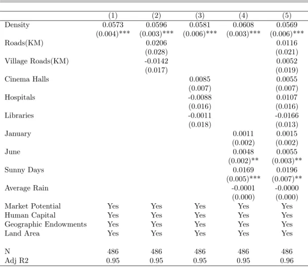
Table 6 presents the 2SLS results.32 For comparability, I start by presenting the OLS and 2SLS
results where density is the only explanatory variable. Column 1 presents OLS results for all provinces. Column 2 presents OLS results where 3 provinces for which instrument is not available are excluded. The elasticity hardly changes. Column 3 presents 2SLS results where density is instrumented with population density in 1914 and growth in population density between 1914 and 1927. In Column 4 and 5, I add domestic market potential, which I instrument using the domestic market potential in 1945. Introduction of this additional variable does not change the elasticity of density. In Columns 6 and 7, I include the human capital control which lowers the magnitude of both density and domestic market potential. This points to the relatively unequal distribution of the share of high skilled individuals, and a relatively strong correlation between employment density and human capital (Pearson’s R ≈ 0.44). In addition to the instruments used in the previous regressions, I add the number of enrolled male students in 1927 as an additional instrument. This positive and significant effect is expected as it captures both the private gains due to skills and the externalities generated by the presence of higher skilled individuals in an
agglomeration.33
In Columns 8 and 9, I further control for the land area and diversity of the local economic activity. Although the former can be considered exogenous to density, the latter is correlated. The coefficient of the land area is statistically significant, and suggests that for a given level of density, an increase in the land area increases the average productivity. If, for example, the land size of a province doubles, the
31I have a broader set of possible instruments, and I experimented with multiple combinations. I have a broader set of
possible instruments, and I experimented with many combinations, all of which yielded broadly consistent results with one another and with the OLS. I report estimations using the same sets of instruments to allow for reliable comparisons. I also try to be restrictive about the number of instruments and use just enough to carry out over-identification tests. Results using other sets of instruments are availabe if requested.
32Appendix H1 table reports the first-stage results.
33The coefficient on the share of high skilled workers will also capture complementarities between skilled and unskilled
labor in the production function. Also, as more educated workers flock to cities with higher wages, it also adds to the identification issues. Controlling for human capital make progress towards the identification of the true elasticity of density but also make it possible to compare it with the findings in the literature.
wages increase around 3%. The diversity, on the other hand, is insignificant which is quite common in the literature (Combes and Gobillon, 2015).
Finally, I account for endowments. As discussed earlier, many productive endowments (such as
airports, high-speed train lines, highways) can increase wages. However, given the endogeneity concerns in using such controls, I consider only four (exogenous) endowment variables that are related to the geography and thus are less concerning in terms of endogeneity. In Columns 10 and 11, I include controls to account for differences in length of seashores within the provincial boundaries (Shores), access to sea
coast (Coast ), mean annual temperature (Climate) and presence of rivers (Rivers).34 Compared to the
previous columns, the inclusion of these controls does not impact the other coefficients. The coefficient
of Coast is positive and significant, suggesting that having access to the shore improves productivity.35
While the Shores and Rivers do not seem to have any effect, the Climate seems to decrease productivity.
Overall, the inclusion of these variables do not increase the explanatory power of the regressions (R2)
which is already high.
The last column (11) is my preferred specification, as it is the most comprehensive one. It includes controls that account for skills-based endowments (Human Capital), between-industry interactions (Den-sity, DMP, Human Capital and Land Area) and amenities (Shore, Coast, Climate and Rivers). Den(Den-sity, domestic market potential, and human capital are instrumented with long-lagged variables. The results pass all the relevant statistical test, and the model has high explanatory power.
The elasticity of density is 0.057, which is exactly the same as those found in Table 3. The domestic market potential remains positive and highly significant. The estimated coefficient (0.1) is a little less than the double of density, suggesting that having access to other markets is the most important deter-minant of the productivity differences across Turkish provinces. If the market potential of a province doubles (e.g., employment density doubles in all other provinces), the wages increase by 6.5%. This number is more than the triple of the 0.02 found for France in Combes et al. (2008), but smaller than
0.13-0.22 found for China in Combes et al. (2020).36 Once instrumented, human capital spillovers
be-comes statistically insignificant. When the same regression is estimated without density, the coefficient on human capital is high and significant. Given the high correlation between the two variables (Pearson’s
R ≈ 0.44), it is possible that the effect of human capital is captured by density.37
34I drop diversity as it is insignificant and generates unnecessary endogeneity.
35It is important to note that this variable captures the walking distance to the closest seashore. It does not imply having
access to a port, which would be highly endogenous.
36The impact of market size on wages has been studied for China (Au and Henderson, 2006), India (Lall et al., 2004),
and Colombia (Duranton, 2016). Theses studies also find that market size has a larger effect than in developed countries.
37The mixed results regarding human capital externalities is not unusual for developing countries (Duranton, 2016). Still,
to check whether these results are driven by any of the choices made when estimating the regression, I make several tests: First, I instrument human capital with alternative instruments such as the number of enrolled female students in 1927, schools to population ratio in 1927, schools to students ratio in 1927, share of high school in 1985. Second, in case the share of educated population in province population is not used with an appropriate functional form, I use the log of human capital variable. Third, I use alternative human capital measures which go from the more restrive (university degree) to the least restrictive (post-secondary education). In all instances, results and elasticities for all variables hold while the human capital remain positive yet statistically insignificant. Results are available if requested.
5.3
Additional results: Infrastructure and other amenities
In this section, I extend the number of controls used in the previous section and add three sets of variables that can impact the wages: transport infrastructure, cultural and additional set of climatic amenities. The infrastructure amenities (e.g., road infrastructure, train-lines or airports) can improve the productivity by affecting the growth of urban areas, increasing trade and lowering cost of transportation
(Redding and Turner, 2015). Although better infrastructures can improve overall productivity and
increase wages, it can also reduce them through improving market access (thus lowering the prices of inputs and goods). The final effect on the wages is therefore, ambiguous. The literature on the effects of infrastructure is limited, mainly due endogeneity issue making it difficult to establish a causal effect. Cultural amenities such as cinema halls, theaters or parks, can also impact the wages as they may increase the willingness of consumers to pay for land and thus imply higher local land rents (Roback, 1982). When the local prices increase, firms use relatively less land, which in turn can decrease the marginal product of labor, especially if the latter and land are not perfect substitutes. Similarly, amenities related to climate can also have a similar effect as it may increase the cost of land and living through higher housing prices and lower wages (Glaeser and Gottlieb, 2009).
[Table 7 about here.]
Table 7 reports the OLS results where I augment the model in Section 5.2 with additional controls. In all of the regressions I control for market potential, human capital, geographic endowments, land area and include time fixed-effects.
Column 1 replicates the results from Table 6 for comparison. In Column 2, I account for the length of provincial road network (Roads) and village roads (Village Roads). The results suggest that a denser
road network does not impact the wages.38 As discussed earlier, better road networks can impact both
positively and negatively the average wages. The non-significance of the results could be due to two
opposing effects canceling each other out, and does not prove the absence of an effect.39 It should also
be noted that these coefficients capture the effects that remain when controlling for domestic market potential.
In Column 3, I control for cultural amenities and health facilities. The number of cinema halls and libraries have the expected negative sign, although only the former is weakly significant (at 20% signif-icance level). Hospitals, on the other hand, have a positive sign yet is insignificant. The interpretation of this sign is also should be done with caution. While better hospitals can increase the demand for the
location, it can also be the consequence of higher levels of local income.40
38It should be noted that provincial and village roads are inferior to highways. While village roads are correlated with
lower densities and rural economic structure, the relationship between provincial roads and density follows an inverse U-shape. That is why attempts to establish a linear relationships should be addressed with caution. Although not reported here, the highway network, which was very limited in the period of analysis, does not change results and remain insignificant.
39For more on the issue, see Duranton (2016).
40Although not reported, I also tested for other amenities such as the number of theaters, museums, doctors, clinics, the


![[PDF] Le mécanisme d’exception du langage Java | Cours informatique](data:image/gif;base64,R0lGODlhAQABAIAAAP///wAAACH5BAEAAAAALAAAAAABAAEAAAICRAEAOw==)