HAL Id: hal-00488716
https://hal.archives-ouvertes.fr/hal-00488716
Preprint submitted on 2 Jun 2010
HAL is a multi-disciplinary open access
archive for the deposit and dissemination of sci-entific research documents, whether they are pub-lished or not. The documents may come from teaching and research institutions in France or abroad, or from public or private research centers.
L’archive ouverte pluridisciplinaire HAL, est destinée au dépôt et à la diffusion de documents scientifiques de niveau recherche, publiés ou non, émanant des établissements d’enseignement et de recherche français ou étrangers, des laboratoires publics ou privés.
concentrations for the early universe reconstruction
problem
Yann Brenier
To cite this version:
Yann Brenier. A modified least action principle allowing mass concentrations for the early universe reconstruction problem. 2010. �hal-00488716�
CONCENTRATIONS FOR THE EARLY UNIVERSE RECONSTRUCTION PROBLEM
YANN BRENIER
Abstract
We address the early universe reconstruction (EUR) problem (as considered by Frisch and coauthors in [24]), and the related Zeldovich approximate model [39]. By substi-tuting the fully nonlinear Monge-Amp`ere equation for the linear Poisson equation to model gravitation, we introduce a modified mathematical model (”Monge-Amp`ere gravi-tation/MAG”), for which the Zeldovich approximation becomes exact. The MAG model enjoys a least action principle in which we can input mass concentration effects in a canonical way, based on the theory of gradient flows with convex potentials and some-what related to the concept of self-dual Lagrangians developped by Ghoussoub [27]. A fully discrete algorithm is introduced for the EUR problem in one space dimension.
Introduction
This paper addresses the early universe reconstruction (EUR) problem discussed by Frisch and coauthors in [24, 17]. We refer to these papers for the detailed physical back-ground of this important problem in cosmology. Here is a simplified mathematical for-mulation.
We consider (for simplicity) a smooth closed bounded 3D domain D ⊂ R3 and denote
the space variable by x ∈ D. We are given two times t1 > t0 > 0, two probability
mea-sures ρ0(dx), ρ1(dx) on D. We look for a time-dependent family of probability measures
ρ(t, dx) on D (depending continuously on the time variable t, with respect to the weak convergence of measures), interpolating ρ0 and ρ1, at t = t0 and t = t1 respectively, and
minimizing the following action
(0.1) Z t1 t0 dt Z D α(t)2ρ(t, dx)|v(t, x)|2+ β(t)2|∇ϕ(t, x)|2 dx ,
where v = v(t, x) ∈ R3 is a vector-field and ϕ = ϕ(t, x) a scalar field, respectively subject
to:
(0.2) ∂tρ + ∇ · (ρv) = 0 , ρ = 1 + ∆ϕ .
Here ∆ = ∇2 is the Laplace operator. In the definition of the action, α and β are
time-dependent scaling parameters related to general relativity (GR). Following [24, 17] (case of an Einstein-de Sitter universe), we set:
(0.3) α(t) = t3/4, β(t) = t−1/4p3/2 .
The formal optimality conditions read (0.4) v = v(t, x) = ∇θ(t, x) α(t)2 , ∂tθ + |∇θ|2 2α2 + β 2ϕ = 0 ,
which can be also (still formally) written:
(0.5) ∂t(α2v) + α2(v · ∇)v = −β2∇ϕ , ∇ × v = 0 ,
or
(0.6) ∂t(α2ρv) + ∇ · (α2ρv ⊗ v) = −β2ρ∇ϕ , ∇ × v = 0 .
These equations, namely (0.2,0.6) are (up to the scaling factors α, β which come from general relativity) nothing but the Euler-Poisson equations for a pressure-less, curl-free, self-gravitating gas subject to classical Newton gravitation. These equations can also be written, using ”material coordinates” ,
(0.7) ∂t(α(t)2∂tX(t, a)) = −β(t)2(∇ϕ)(t, X(t, a)),
where a denotes the material coordinate, X(t, a) the position at time t of the mass particle with label a. In the case of coefficients (0.3), we find
(0.8) 2t 3∂ 2 ttX(t, a) + ∂tX(t, a) = −(∇ ˜ϕ)(t, X(t, a)), where ˜ϕ(t, x) = ϕ(t, x)/t satisfies ρ = 1 + t∆ ˜ϕ.
Remarkably enough, at early stage t << 1, the density field must be uniformly equal to 1 (otherwise solutions are unbounded) and, even more surprisingly, the acceleration term is dominated by the velocity term, due to general relativity! (In some sense, Newton modified by Einstein returns to Aristoteles.) As a consequence, an amazingly simple approximate formula was proposed by Zeldovich [39]:
(0.9) X(t, a) = a − t∇ ˜ϕ0(a),
where ˜ϕ0 is related to the behavior of the density field ρ(t, ·) at early stages
ρ(0, x) = 1, ∆ ˜ϕ0 = lim t↓0
ρ(t, x) − 1 t .
The Zeldovich approximate formula suggests possible mass concentrations in finite time. Indeed, denoting by Λ the largest eigenvalue of the Hessian matrix D2ϕ˜
0(a), for all a, we
see that, whenever Λ > 0, the map a → X(t, a) is no longer invertible at t = Λ−1. Beyond
the concentration time, there are many possibilities of extending the formula and this is still a controversial issue from the physical viewpoint. It depends very much on whether or not we want to prevent interpenetration of particles. If we do so, we are naturally lead to the model of adhesion dynamics, where particles merge after collisions, which is the most possible dissipative behavior beyond concentrations. (See [5, 23, 24].) This issue can be simply addressed in terms of nonlinear hyperbolic PDEs [22]. Indeed, given a Zeldovich solution X defined by (0.9), let us introduce the field u(t, x) implicitly defined by:
(0.10) u(t, X(t, a)) = a − X(t, a)
as long as a → X(t, a) stays smooth and invertible. Then, we see that u solves the multidimensional ”invisicid Burgers” equation
(0.11) ∂tu + (u · ∇)u = 0.
In one space dimension, if we want a global solution for all times, the monotonicity condition ∂aX(t, a) ≥ 0 exactly corresponds to “Oleinik’s entropy condition” ∂xu ≤ 1/t,
which guarantees both global existence and uniqueness for solutions of the inviscid Burgers equation (0.11), written in ”conservation form”
(0.12) ∂tu + ∂x(
u2
2 ) = 0.
Going back to the least action principle, it is remarkable that action (0.1) is (strictly) convex in the variables (ρ, ρv, ϕ), while the differential constraints (0.2) are linear in these variables. With classical tools of convex and functional analysis, Loeper [30] was able to prove the existence of a unique minimizer in the class of probability measures ρ(t, dx) which have no singular part with respect to the Lebesgue measure, i.e. without concentrations, provided the data ρ0 and ρ1 are themselves concentration-free. [He also
rigorously derived optimality conditions (0.6).] This existence and uniqueness result is quite remarkable. However, it provides only solutions to the Euler-Poisson system with-out concentrations. This is a major defect, since the initial value problem (as both ρ and v are prescribed at initial time t0) is expected to have solutions with concentrations
appearing in finite time, for most initial conditions. So, minimizing action (0.1) under constraints (0.2) is not a fully satisfactory way to recover solutions of the EP system from the knowledge of ρ0 and ρ1. The goal of the present paper is to investigate how the action
can be modified so that its minimizers are not necessarily concentration-free. A similar problem, in the framework of adhesion-fragmentation processes, has been recently solved by Wolansky [38]. (See also the pioneering work of Shnirelman [35] for sticky particles and adhesion dynamics.) Our approach is different and more reminiscent of the recent theory of self-dual lagrangians by Ghoussoub [27]. Unfortunately, it does not apply to the desired Euler-Poisson system but rather to the modified system obtained by substi-tuting the fully nonlinear Monge-Amp`ere equation ρ = det(I + tD2
xϕ), for the Poisson˜
equation ρ = 1 + t∆ ˜ϕ (in case of coefficients (0.3)). Notice that these systems agree for solutions depending only on one spatial coordinate (i.e. with sheet structure) and are asymptotically close for t << 1. Of course, changing the model is not a satisfactory approach, without further justification. Our main argument is the following remarkable property of the resulting Euler-Monge-Amp`ere system: it admits as exact solutions the Zeldovich approximate solutions (0.9). As a secondary justification, let us recall that the Euler-Poisson system is, after all, itself an approximation of the full Einstein equations and it might be, from this viewpoint, equally good to use the Monge-Amp`ere equation and the Poisson equation. [A similar situation occurs in fluid mechanics when comparing the quasi-geostrophic and the semi-geostrophic approximations of the Euler equations for ocean and atmosphere dynamics, as discussed in [21]. See also [18].] However, there will be no attempt in the present paper to justify this last statement.
In the first section, we introduce a family of infinite dimensional dynamical systems, in a rather abstract (but straightforward) framework, requiring a limited amount of classi-cal functional analysis (Hilbert spaces) and elementary convex analysis (sub-differential calculus). Then, the ”Monge-Amp`ere” gravitation (MAG) model is introduced as a par-ticular case. The model is first described in ”material variables” and then translated into ”Eulerian variables”, leading to a pressure-less Euler-Monge-Amp`ere system of PDEs. In section 2, we return to the abstract framework and observe that the potential part of the action has the very special property to be a squared distance function. This allows a rewriting of the action as an exact square and we find as special minimizers all the solutions of the gradient flow equation associated to the potential. [This special solutions play more or less the same role as ”instantons” in Yang-Mills theory [27].] It turns out that this gradient flow belongs to a very well-studied class of evolution equations, linked to the theory of ”maximal monotone operators” [19]. This suggests a somewhat canonical modification of the action.
In section 3, we adapt the previous discussion to Monge-Amp`ere gravitation and get a modified action that takes into account concentrations. Then, we observe that the solu-tions of the gradient flow equation exactly are the Zeldovich approximate solusolu-tions (0.9) of the Euler-Poisson system, which, in some sense, justifies the MAG model as a reason-able approximate model.
In section 4, we introduce a fully discrete algorithm to compute the EUR problem with Monge-Amp`ere gravitation.
In section 5, we introduce a numerical scheme for the initial value problem and, finally, in section 6, we provide numerical results in the very special case of one space variable.
1. The abstract framework
Let H be a (separable) Hilbert space H equipped with its norm denoted || · || and the corresponding inner product ((·, ·)). We first consider the general dynamical system
(1.13) d
2X
dt2 = (∇HΦ)[X],
where t → X(t) is valued in H, ∇H denotes the gradient operator in H, and Φ is a given
”potential” defined on H. (Observe that we do not follow the usual sign convention for the potential, for notational convenience.) As well known, such a system admits a least action principle, at least at a formal level. Indeed, for a curve t → X(t) valued in the Hilbert space H, we may define its action between times t0 and t1, t1 > t0 by:
(1.14) A[t0,t1][X] = Z t1 t0 1 2|| dX dt || 2+ Φ[X(t)] dt.
Then, the dynamical equation (1.13) can be seen as the formal optimality equation ob-tained by minimizing the action (1.14) as the end points X(t0) and X(t1) are fixed.
Next, we crucially assume the potential to be of form:
(1.15) Φ[X] = inf{||X − s||
2
2 ; s ∈ S},
where S is a given bounded subset of H. Then, when it makes sense, X − ∇HΦ[X] is just
X has several distinct closest points, which may happen unless S is a convex set. In some cases, X may have no closest point in S!) As a consequence, (1.13) formally means:
(1.16) d
2X
dt2 = X − π[X],
where π[X] is the closest point to X on S. With this formulation, we can guess a large class of explicit solutions. Indeed, let us assume that X(0) = X0 has a unique closest
point π[X0] = π0 on S. Then the linear (but not convex) combination of X0 and π0 given
by:
(1.17) X(t) = π0+ et(X0− π0)
solves (1.16) as long as π0 stays the unique projection of X(t). Intuitively, X(t) gets
repelled from its initial position in the opposite direction of its closest point on S, keeping for a while π0 as its closest point on S until a new point in S gets even closer. Whenever
S is a convex set, this repulsion mechanism provides an obvious global solution. Indeed, all points contained in the infinite segment {π0+ r(X0− π0), r ≥ 0} admits π0 as their
unique closest point on S. In the case of a non-convex set S, this is not true in general and formula (1.17) is able to provide no more than a local solution. The situation is very clear in the elementary case when S is the unit sphere in H. Then, 0 is the unique point where Φ is not differentiable. We get as special solution
X(t) = r0−1(1 + (r0− 1)et)X0,
where X0 6= 0 and r0 = ||X0||. We see that, if r0 < 1, then the solution reaches 0 at time
T = − log(1 − r0) and its continuation beyond T gets ambiguous.
Miscellaneous mathematical remarks. 1) The potential Φ given by (1.15) is a smooth perturbation of a Lipschitz concave function; indeed:
(1.18) Φ[X] = ||X||
2
2 − Π[X], where Π is the Lipschitz convex functional defined by:
(1.19) Π[X] = sup{((X, s)) − ||s||
2
2 ; s ∈ S}.
A classical result of convex analysis [4] asserts that, for every Lipschitz convex function defined on a Hilbert space, the set ˜H where the function is differentiable is always ”fat” in the topological sense of Baire: namely ˜H is dense and contains a countable intersection of dense open subsets of H [4]. In the particular case of Π, the set of differentiabliity
˜
H is contained in the set of all points X in H for which there is a unique closest point s = π[X] on S. Thus, the potential Φ defined by (1.15) is everywhere differentiable on ˜H and its gradient in H is given by:
(1.20) ∇HΦ[X] = X − π[X], ∀X ∈ ˜H.
2) In the case when H is the finite-dimensional Hilbert space Rn, for such a
poten-tial (namely a smooth perturbation of a concave Lipschitz function), the dynamical system (1.13) has a unique global solution for Lebesgue almost every initial condition (X(0), X′
[8, 1]. To the best of our knowledge, there is no similar theory in infinite dimension and the well-posedness of (1.13) is then a challenging open. (A somewhat related attempt is the theory developed by Ambrosio and Gangbo for some infinite dimensional hamiltonian systems [2]. See also [18, 25, 26].)
1.1. Monge-Amp`ere gravitation.
Definition. Since the dimension 3 does not matter in the definition of the MAG model, we consider a smooth bounded closed domain D ⊂ Rd. We assume D to be of unit Lebesgue
measure. The MAG model is defined by choosing for H the Hilbert space of all Lebesgue square-integrable maps from D to Rd,
(1.21) H = L2(D, Rd),
and for S the subset of all Lebesgue measure-preserving maps s of D: (1.22) S = { s ∈ H , Z D f (s(a))da = Z D f (a)da, ∀f ∈ C(Rd) } .
In addition, with respect to the abstract framework, we input coefficients α, β given by (0.3) and substitute (1.23) β−2(t)d dt(α 2(t)dX dt ) = (∇HΦ)[X] = X − π[X], for (1.13).
Eulerian formulation. We now want to write the MAG model in ”Eulerian coordinates”. Given a solution t → X(t) ∈ H, we introduce the pair of measures (ρ, ρv), respectively valued in R and Rd and defined by:
ρ(t, dx) = Z Dδ(x − X(t, a))da, v(t, x)ρ(t, dx) = Z D ∂tX(t, a)δ(x − X(t, a))da. (1.24)
Using the tools of ”optimal transportation theory” [11, 12, 37] (cf. Appendix), we (for-mally) get for (ρ, v) the following system of partial differential equations:
∂tρ + ∇ · (ρv) = 0, ∂t(α2ρv) + ∇ · (α2ρv ⊗ v) = −β2ρ∇ϕ , ρ = det(I + D2xϕ), (1.25) where (ρ, v, ϕ)(t, x) ∈ R+× Rd× R, (t, x) ∈ R × Rd, I = (δij), D2x= (∂x2ixj).
Thus our model can be seen as a nonlinear correction of the classical pressure-less Euler-Poisson system (EP), obtained by substituting the fully nonlinear Monge-Amp`ere equa-tion
(1.26) ρ = det(I + Dx2ϕ). for the linear Poisson equation
For this reason, we call Monge-Amp`ere gravitation (MAG) the model defined by either (1.16,1.21,1.22) or (1.25). Notice that the MAG model coincides with the conventional Euler-Poisson model in dimension d = 1.
2. Modified action in the abstract framework
In this section, we go back to the abstract framework of a potential Φ defined as the squared distance to a bounded subset S of a general Hilbert space H, according to (1.16,1.18,1.19).
2.1. The self-dual form of the action. Since potential Φ is a squared distance to some subset S inside H, it solves, at least formally, the stationary Hamilton-Jacobi equation:
(2.28) Φ = ||∇HΦ||
2
2 ,
where ∇H denotes the gradient operator in H. This suggest to rewrite, at least formally,
the action (1.14) as Z t1 t0 1 2|| dX dt || 2+||∇HΦ[X(t)]||2 2 dt = Z t1 t0 1 2|| dX dt − ∇HΦ[X(t)]|| 2+ ((dX dt , ∇HΦ[X(t)])) dt = Φ[X(t1)] − Φ[X(t0)] + Z t1 t0 1 2|| dX dt − ∇HΦ[X(t)]|| 2 dt. (2.29)
Under this ”self-dual” form (see [27] for a systematic study of ”self-dual lagrangians”), it is obvious that any solution of
(2.30) dX
dt = (∇HΦ)[X] = X − (∇HΠ)[X]
is always a minimizer of the action as X(t0) and X(t1) are fixed (just like instantons in
euclidean Yang-Mills theory, cf.[27]).
2.2. A gradient flow equation. As already mentioned, in spite of the rather nice struc-ture (1.18) of Φ, as a quadratic perturbation of a convex Lipschitz function, the corre-sponding second-order equation (1.16) is not so well understood. In sharp contrast, the first-order equation (2.30) is a standard ”gradient flow ” equation (GF), that can be solved by classical ”maximal monotone operator” theory [19].
In the framework of maximal monotone operator theory, equation (2.30) is usually written as a sub-differential inclusion:
(2.31) −dX
dt + X ∈ ∂Π[X],
which is well-posed in H since Π is Lipschitz and convex. Here, we use standard notations of convex analysis, for which ∂ denotes the sub-differential of a convex function [19]: (2.32) ∂Π[X] = {Z ∈ H; Π[Y ] ≥ Π[X] + ((Z, Y − X)), ∀Y ∈ H}.
A remarkable property [19] of each solution X(t) ∈ H is to be not only a Lipschitz continuous function of t but also right-differentiable at each t with
(2.33) −dX(t + 0)
dt + X(t) = d
0Π[X(t)],
∀ t
where d0Π[X], following [3], denotes the element of ∂Π[X] with minimal norm (which is
uniquely defined):
(2.34) ||d0Π[X]|| = min{||s|| ; s ∈ ∂Π[X]}.
Finally, notice that X(t) is a locally Lipschitz function of t with values in the separable Hilbert space H, X(t) is therefore almost everywhere differentiable in t by Rademacher theorem. Since X(t) is right-differentiable everywhere, we conclude that:
(2.35) −dX
dt + X(t) = d
0Π[X(t)],
holds true both in the almost everywhere sense and in the sense of distributions.
2.3. Proposals for a modified action. Our main point is now to introduce a modif ied action. There are two possible ways to do it. First, we may introduce the modified potential ˜Φ:
(2.36) Φ[X] =˜ 1
2||X − d
0
Π[X]||2 and the corresponding modified action
(2.37) ˜A[t0,t1][X] = Z t1 t0 1 2|| dX dt || 2+ ˜Φ[X(t)] dt = Z t1 t0 1 2|| dX dt || 2+1 2||X − d 0 Π[X]||2 dt. Alternately, sticking more closely to the self-dual formulation, we may directly modify the action by setting
(2.38) Aˆ[t0,t1][X] = Z t1 t0 1 2|| dX dt − X + d 0 Π[X]||2 dt.
It is not clear to us that these modified actions coincide (up to boundary terms). Nev-ertheless, we will take the second option, mostly for numerical purposes, because it leads to simpler algorithms.
3. Application to the EUR problem with Monge-Amp`ere gravitation We now address the Monge-Amp`ere gravitation (MAG) model and the EUR problem. This means, with respect to the abstract framework, that H and S are now defined by (1.21,1.22) and (1.23) substitutes for (1.13).
3.1. A modified action for the EUR problem. In order to take into account coeffi-cients (α, β) (given by (0.3)), we first rewrite the action as:
(3.39) A = Z t1 t0 α(t)2||dX dt || 2+ β(t)2 ||∇HΦ[X(t)]||2 dt .
As in the homogeneous case α = β = 1, we keep in mind that 1
2||∇HΦ[X(t)]||
2
= Φ[X(t)]| and look at the cross-term:
J = Z t1 t0 α(t)β(t)((dX dt , ∇HΦ[X(t)]))dt = Z t1 t0 α(t)β(t)d dt(Φ[X(t)])dt By integration by part, we get
J − α(t1)β(t1)Φ[X(t1)] + α(t0)β(t0)Φ[X(t0)] = − Z t1 t0 Φ[X(t)] d dt(α(t)β(t))dt = −1 2 Z t1 t0 ||∇HΦ[X(t)]||2 d dt(α(t)β(t))dt = − λ 2 Z t1 t0 β(t)2||∇ HΦ[X(t)]||2, provided we assume (3.40) d dt(α(t)β(t)) = λβ(t) 2,
for some constant λ, which is is consistent with data (0.3) if we choose λ = 1/√6. From this calculation of the cross-term J, we deduce that the action A defined by (3.39) can be written: A = BT + Z t1 t0 ||α(t)dX dt − µβ(t)∇HΦ[X(t)]|| 2 dt .
where BT is a boundary term depending only on X(t1) and X(t0), provided µ2+ µλ = 1.
For data (0.3), we get λ = 1/√6 and µ =p2/3. Therefore, all solutions of the gradient-flow equation
(3.41) α(t)dX
dt = µβ(t)∇HΦ[X(t)]
automatically are minimizers of the action (3.39). For data (0.3), this gradient-flow equa-tion reduces to:
(3.42) t dX
dt = ∇HΦ[X(t)] = X(t) − ∇HΠ[X(t)].
The gradient-flow equation should be understood in the more precise sense:
(3.43) t dX(t + 0)
dt = X(t) − d
0Π[X(t)],
which takes concentration into account, globally in time. In some sense, formulation (3.43) not only allows concentrations but guarantees the largest possible dissipation of kinetic energy during the concentration process (which is of course questionable from the
physical viewpoint.) Accordingly, we suggest, for the EUR problem with Monge-Amp`ere gravitation, the following modified action:
(3.44) A =ˆ Z t1 t0 t−1/2||tdX dt − X + d 0 Π[X]||2 dt.
3.2. Zeldovich solutions. Special solutions of (3.42) can be obtained thanks to the concept of ”rearrangements with convex potential” as follows. By definition, the MAG model relies on the set S of all Lebesgue measure-preserving maps (1.22). This set contains the identity map Id as an obvious element. The set K ⊂ H of all points X which admits Id as a closest point on S plays a crucial role. It can be characterized (cf. Appendix on optimal transportation theory), as the convex cone of all maps X ∈ H with a convex potential, which means that there is a convex function ψ defined on Rd and valued in
] − ∞, +∞] which is almost everywhere differentiable on D with ∇ψ(a) = X(a), a.e. on D. It turns out that any map X ∈ H has a unique rearrangement X♯ in K, which means
Z Dδ(x − X ♯(a))da = Z Dδ(x − X(a))da (cf. Appendix).
Therefore, special solutions of (3.42) can be obtained, by looking for solutions X(t) valued in the convex cone K of all maps with convex potential. Indeed, for such solutions, we have:
∇HΦ[X(t)] = X(t) − ∇HΠ[X(t)] = X(t) − π[X(t)] = X(t) − Id,
and (3.42) reduces to the linear ODE
(3.45) t dX
dt = X − Id
as long as X(t) belongs to K, i.e. X(t, a) = ∇ψ(t, a), with ψ(t, a) convex in a. This leads to the explicit formula:
(3.46) X(t, a) = ∇ψ(t, a) = a + t t0(∇ψ(t 0, a) − a) = a + t t0 (X(t0, a) − a) ,
as long as ψ stays convex in a. This exactly coincides with Zeldovich formula (0.9) dis-cussed in the introduction. Remarkably enough, for Monge-Amp`ere gravitation, Zeldovich approximation (0.9) is just exact!
3.3. Modified action in one space dimension. Let us focus on the one space di-mension case when: D = [−1/2, 1/2]. Then, the modified potential ˜Φ can be explicitly computed in the case of a piecewise smooth map Y valued in K. Indeed, in one space dimension, maps in K, with convex potential are just increasing maps. So, there is a finite number of plateaux [aj, bj] on which Y is constant with values Yj and outside of
which Y is a piecewise smooth strictly increasing function. Notice that the corresponding image-measure ρ(dx) defined by
ρ(dx) = Z
has a singular part ρs given by:
ρs(dx) =
X
j
(bj− aj)δ(x − Yj).
Then d0Π[Y ] (the element of the sub-differential ∂Π[Y ] with minimal L2 norm) coincides
with the identity map outside of the plateaux and takes value (aj + bj)/2 inside [aj, bj].
After elementary calculations, we find
||Y − d0Π[Y ]||2 = ||Y ||2− 2((Y, Id)) + ||Id||2−X
j Z bj aj (a −aj + bj 2 ) 2da = ||Y − Id||2−121 X j (bj− aj)3.
Here we very clearly see the discrepancy between the original potential Φ and the modified potential ˜Φ: (3.47) Φ[Y ] = Φ[Y ] −˜ 1 24 X j (bj − aj)3.
Remark. Specialists of nonlinear hyperbolic conservation laws will recognize in the second term of this expression the very expression of the so-called ”entropy production” term for the inviscid Burgers equation (0.12), written in material coordinates [6, 22].
3.4. Eulerian formulation of the gradient flow equation. The gradient flow equa-tion (3.41) has an Eulerian version. Indeed, the corresponding measures (ρ, ρv), defined by (1.24), are (formal) solutions of the following system of PDE:
(3.48) ∂tρ − ∇ · (ρ∇ ˜ϕ) = 0, ρ = det(I + tDx2ϕ),˜
where ˜ϕ(t, x) = ϕ(t, x)/t. This model can be seen as a fully nonlinear counterpart of vari-ous models popular in biology (chemotaxis) or astronomy, involving the Poisson equation -or other linear equations involving a singular Green function- rather than the Monge-Amp`ere equation. A common feature of all these models is their ability at describing concentration phenomena [29, 28, 33, 20].
4. The discrete EUR problem with Monge-Amp`ere gravitation
4.1. A time-discrete scheme for the gradient flow equation. In view of numerical calculations, our first step is to get a time-discrete version of the modified action. Instead of directly getting a discrete version of (3.44), it seems wiser to us to start from a time-discrete version of the gradient flow equation (3.42).
A natural candidate is:
(4.49) Xn+1 = Xn(1 + θn) − ∇HΠ[Xn]θn+ ηn
where Xn is an approximation of X(t) at the nth time-step Tn, for n = 0, · · ·, N, T0 = t0,
TN = t1, with θn = Tn+1Tn − 1 ↓ 0. Here ηn is a small perturbation added to the discrete
solution so that, for every n, Xnis a point of differentiablity of Π. Thus, ∇HΠ[Xn] is well
defined and is also the closest point π[Xn] to Xn in S. Indeed, as a smooth perturbation
of a Lipschitz concave function on H, Π is differentiable on a ”fat” dense subset ˜H of H (i.e. containing a countable intersection of dense open sets). Thus, we may choose a
perturbation term ηn, arbitrarily small, so that Xn falls in the ”good” set ˜H where ∇HΠ
is well defined. By doing so, we do not generate a big error. Indeed, we keep control on the cumulated error thanks to the following stability estimate for two distinct solution Xn,
˜
Xn of (4.49) (where we neglect the perturbation terms ηn, ˜ηn for notational simplicity),
(4.50) ||Xn+1− ˜Xn+1||2 ≤ (1 + θn)2||Xn− ˜Xn||2+ c0θ2n,
where c0 is the squared diameter of S. [Indeed, we get form (4.49)
||Xn+1− ˜Xn+1||2 = (1 + θn)2||Xn− ˜Xn||2− 2(1 + θn)θn((Xn− ˜Xn, ∇HΠ[Xn] − ∇HΠ[ ˜Xn]))
+θn2||π[Xn] − π[ ˜Xn]||2
and observe that the second term in the right-hand side is less than zero since Π is convex, and the third one is dominated by c0θn2.]
As a matter of fact, this stability estimate is also essentially sufficient to prove the conver-gence of the scheme as θn↓ 0 to the continuous model (3.43), for the uniform convergence
in time with respect to the strong topology of H. (See [13, 14] for examples of similar results for various nonlinear hyperbolic conservation laws.) Notice that concentration phenomena, which are present at the continuous level, are correctly taken into account by the time discrete scheme, in spite of the fact that the discrete scheme never involves the computation of d0Π, which is a big advantage in practice!
4.2. The time-discrete EUR problem with Monge-Amp`ere gravitation. From the time-discrete scheme (4.49) for the gradient-flow equation, we define a time discrete version of modified action (3.44) just by setting:
(4.51) N −1 X n=0 rn||Xn+1− Xn(1 + θn) + π[Xn]θn||2, with rn = T 3/2 n
Tn+1−Tn. Nevertheless, minimizing the time-discrete action (4.51), as both X0
and XN are fixed, is not really consistent with the original EUR problem, where the data
are not X0 and XN but rather the corresponding probability measures ρ0 and ρN defined
by: ρ0(dx) = Z Dδ(x − X 0(a))da, ρN(dx) = Z Dδ(x − X N(a))da.
So there is a big loss of information (since the same probability measure can be generated by a continuum of maps). This problem can be addressed in terms of rearrangements with convex potentials. As a matter of fact, fixing ρ0 and ρN is equivalent to fixing the
rearrangements with convex potentials X0♯ and XN♯ , rather than X0 and XN themselves.
It is very fortunate that, one can rewrite the discrete scheme (4.49) as a self-consistent scheme for the rearrangement Yn = Xn♯ with convex potential. Indeed, let us assume,
for simplicity, that, at each n, the solution of the scheme Xn has a polar factorization
Xn = Yn ◦ sn (cf. Appendix), where Yn = Xn♯ ∈ K is the unique rearrangement with
convex potential of Xn and sn = π[Xn] ∈ S is the closest point in S to Xn. Then, we can
rewrite (4.49) as:
But, this implies that Yn+1is the unique rearrangement of Yn(1 + θn) −θnId with a convex
potential. In other words, we have a well defined self-consistent scheme for Yn ∈ K,
namely:
(4.52) Yn+1 = (Yn(1 + θn) − θnId)♯.
Accordingly, the time discrete EUR problem with Monge-Amp`ere gravitation can be seen, in ”polar coordinates” (Yn, sn) ∈ K × S, as the minimization of
(4.53) N −1 X n=0 rn||Yn+1◦ sn+1− (Yn(1 + θn) − θnId) ◦ sn||2, with rn= T 3/2 n
Tn+1−Tn, as Y0 and YN are fixed in K.
Following ”optimal transport” theory, we may introduce on H the quadratic Monge-Kantorovich (MK2) (or ”Wasserstein”) distance,
(4.54) dM K2(X, ˜X) = inf{||X ◦ s − ˜X ◦ ˜s||, s, ˜s ∈ S },
which is nothing but the quotient distance in H with respect to the action of the semi-group S. Then the discrete EUR problem is just the minimization in Yn∈ K of
(4.55) N −1 X n=0 rndM K2(Yn+1, Yn(1 + θn) − θnId)2, with rn= T 3/2 n
Tn+1−Tn, as Y0 and YN are fixed in K.
(Equivalently, we could work on the so-called ”Wasserstein” or ”MK2” space as, for instance, in [34, 3, 2].)
4.3. The fully discrete least action principle. Let us now introduce a fully discrete scheme, for which not only the time variable but also the space variable is discrete. The domain is divided into L disjoints subdomains Diof Lebesgue measure 1/L, for i = 1, ···, L,
with barycenter ai and vanishing diameter as L → ∞. In our abstract framework, it is
enough to substitute for the spatial domain D, the discrete set {ai, i = 1, · · ·, L }.
Accordingly, H can be seen as the euclidean space (Rd)L of all finite sequences of L
points in Rd {X = (X
i ∈ Rd)i=1,L} with the natural euclidean norm || · || induced by Rd.
Meanwhile the set S can be viewed as the set of all permutations s of the L first integers and K is the corresponding cone of all sequences Yi such that
X
i
Yi· (ai− asi) ≥ 0,
for all permutations s. In one space dimension, K is just the convex cone of all increasing sequences of L real numbers.
The time-discrete EUR problem (4.53) makes sense at the fully discrete level without modification. In this discrete setting, S is a group (which is untrue at the continuous level) and each s can be inverted in S. Thanks to the group property of S and the invari-ance of || · || with respect to S, the minimization problem can be further reduced to the
minimization of (4.56) N −1 X n=0 rn||Yn+1− (Yn(1 + θn) − θnId) ◦ σn+1||2,
in Yn∈ K, σn∈ S, as Y0 and YN are fixed in K (just by setting σn+1 = sn◦ s−1n+1 ∈ S).
To solve this minimization problem, a crude strategy is to use Gauss-Seidel type iterations. We denote by (Yk
n, σnk) the approximation of (Yn, σn) at iteration k and time step n. Let
us fix k and n. To get the updated values σk+1
n and Ynk+1, we inductively suppose that
we already know (Yj
m, , σmj ) for all m if j ≤ k and for all m < n if j = k + 1. Then, we
perform the two following steps: i) First step: we get s = σk+1
n by solving the combinatorial optimization problem
(4.57) inf
s∈S||Y k
n+1− (Ynk(1 + θn) − θnId) ◦ s||.
This step is particularly simple in one space dimension and just amounts to sorting in increasing order the finite sequence (Yk
n(1 + θn) − θnId)i, i = 1, · · ·, L. It is much more
challenging in higher dimensions. The best known optimization methods need 0(L3)
elementary operations, which is not satisfactory (see a related discussion in [17]). ii) Second step: we get Y = Yk+1
n by minimizing in Y ∈ K:
rn||Yn+1k − (Y (1 + θn) − θnId) ◦ σn+1k ||2+ rn−1||Y − (Yn−1k+1(1 + θn−1) − θn−1Id) ◦ σnk+1||2,
where the first term can also be written
rn||Yn+1k ◦ (σkn+1)−1− (Y (1 + θn) − θnId)||2,
using the inverse permutation (σk
n+1)−1 and the invariance of || · || with respect to
per-mutations. After reorganizing squares, we see that Y is just the least-square projection H → K of:
V = rn(1 + θn)W + rn−1Z rn(1 + θn)2+ rn−1
,
W = Yn+1k ◦ (σn+1k )−1+ θnId, Z = (Yn−1k+1(1 + θn−1) − θn−1Id) ◦ σk+1n .
So, we have obtained an effective algorithm. It is particularly simple in one space dimen-sion (and much more challenging in higher dimendimen-sions!). Let us observe that, in one space dimension, computing the least-square projection Y = PK[V ] is different from sorting the
sequence V in increasing order. However, still in one space dimension, this projection can be approximately computed after a sequence of sorting steps, according to the asymptotic formula (which is a byproduct of the ”transport-collapse method” [10]):
(4.58) PK[V ] = lim M →∞V M M , VmM = (Vm−1M + 1 MV ) ♯, VM 0 = 0, m = 1, · · ·M.
In practice, we already get a good accuracy for moderate values of M (say M = 10).
5. Solution of the initial value problem
In order to validate the reconstruction scheme, we would like to solve the initial value problem (IVP) consistently with the modified least action problem, and get a discrete scheme for the IVP. Ideally, such a scheme should be derived directly from the modified discrete least action principle. Unfortunately, we have not been able to do so, and we are
just going to suggest a simple scheme for the IVP which seems, in practice, consistent with the modified action, at least in one space dimension.
5.1. A time-discrete scheme for the IVP. Our idea to get a time-discrete solution of the IVP is to alternate the solution of the linear ODE
(5.59) d dt(α
2(t)V ) = β2
(t)(Y − Id), dY
dt = V, Y (Tn) = Yn, V (Tn) = Vn,
with coefficients (α, β) given by (0.3), on each time interval [Tn, Tn+1[ and the
rearrange-ment of the result at time step Tn+1:
Yn+1 = Y (Tn+1)♯, Vn+1= V (Tn+1).
Using a plain explicit discretization of (5.59), we get:
Yn+1= (Yn+ (Tn+1− Tn)Vn)♯,
α2(Tn+1)Vn+1 = α2(Tn)Vn+ β2(Tn)(Tn+1− Tn)(Yn− Id)
(5.60)
The convergence analysis of this time-discrete scheme can be done in two different ways.
5.2. The multidimensional case. In the multidimensional case, our strategy for the convergence analysis of scheme (5.60) is inspired by our recent work [15], where a similar scheme is analyzed. We essentially use the fact that all maps with convex potential are of locally bounded variations, which provides enough compactness with respect to space variables. Time compactness is, as usual, directly obtained from the evolution scheme. We notice that V can be easily integrated out from Y by ODE (5.59).
Theorem 5.1. For every fixed initial condition (Y0, V0) ∈ Y ×H, the approximate solution
(Yn) admits at least a limit t → Y (t) ∈ K valued in C0([t0, +∞[, H) as the time step goes
to zero. This limit satisfies:
V (t, a)α2(t) = V0(a)α2(t0) + Z t t0 β2(τ )(Y (τ, a) − a)dτ, d dt Z D f (Y (t, a))da = Z
D(∇f)(Y (t, a)) · V (t, a)da,
(5.61)
for all C1 function f on Rd (with |∇f| growing at most linearly at infinity).
Notice that, since Y is valued in K, the knowledge of ”observables” R
Df (Y (t, a))da
for all test-functions f is enough to determine Y (t) which makes formulation (5.61) self-consistent. (However this does not guarantee uniqueness of solutions to the IVP.) So, we have a proposal to solve the IVP, and a corresponding discrete scheme, but we are not able to prove that formulation (5.61) is actually consistent with our modified least action principle.
5.3. The one-dimensional case. In the special case of one space variable, we get a much more precise information, following the analysis developed in [13] for similar problems (see also [14]):
Theorem 5.2. For every fixed initial condition (Y0, V0) ∈ Y × H, as the time step goes
to zero, the approximate solution (Yn) converges to the unique solution t → Y (t) ∈ K,
valued in C0([t
0, +∞, H), of the mixed integral-sub-differential system:
−∂tY + V ∈ ∂Θ[Y ], V (t, a)α2(t) = V0(a)α2(t0) + Z t t0 β2(τ )(Y (τ, a) − a)dτ, (5.62)
where Θ[Y ] = 0 whenever Y = Y (t, a) is monotonically increasing in a and Θ[Y ] = +∞ otherwise.
System (5.62) is well-posed in the L2 sense and can be shown (as in [13]) to be the limit
(in the sense of maximal monotone operator theory) as ǫ ↓ 0 of the perturbed system (5.63) −∂tY + V = −ǫ∂a(log(∂aY )), ∂t(α2(t)V ) = β2(t)(Y − Id),
which, in Eulerian variables (1.24), reduces to: ∂tρ + ∂x(ρv) = 0,
∂t(α2(t)ρv) + ∂x(α2(t)ρv2) = −β2(t)ρ∂xϕ + ǫ∂xxv,
ρ = 1 + ∂x2ϕ, (5.64)
and is just a pressure-less Navier-Stokes-Poisson system with vanishing viscosity (as in [9, 36]). As mentioned above, an interesting open question is to show that this approach (vanishing viscosity (5.64), subdifferential formulation (5.62) or scheme (5.60)) is actually consistent with the modified least action principle!
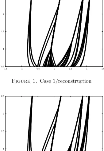
6. Numerical simulations in one space dimension Our data are
t0 = 1/2, t1 = 5/2, N = 60, L = 51, ai = −1 + (2i − 1)/L, i = 1, · · ·L,
Y0 = X0♯, (X0)i = aiωi, ,
where ωi is a random number uniformly distributed between 1 and 2. Thus, Y0 looks like
a devil’s staircase.
Concerning the final data YN ∈ K, either:
(Case 1) the associate probability ρN is the barycenter of four Dirac’s measures:
ρN(dx) = δ(x + 0.7) + 4 δ(x − 0.2) + 3 δ(x − 0.9) + δ(x − 1.1)
9 .
or (Case 2) YN is the solution at time t1 of the initial value problem generated by the
discrete gradient flow equation starting from Y0 = X0♯ at time t0.
In our plots, we draw the trajectories of the 51 particles during the 60 time steps of the time interval (the vertical axis corresponding to time and the horizontal one to space).
Case 1: we first plot the reconstructed solution (fig. 1). Then, with the reconstructed initial velocity we solve the initial value problem for the MAG equations with scheme (5.60) and plot the result (fig.2). We observe a nearly perfect match between figures 1 and 2.
Case 2: we first solve the IVP for the gradient flow equation with scheme (5.60) (fig. 3). Then, we reconstruct the solution from the initial and final data of the gradient flow solution (fig 4). (Here we observe some limited discrepancy.) Finally, with the recon-structed initial velocity we solve the initial value problem for the MAG equations (fig.5), again with scheme (5.60) and get a nearly perfect match.
0.5 1 1.5 2 2.5 -1.5 -1 -0.5 0 0.5 1 1.5
Figure 1. Case 1/reconstruction
0.5 1 1.5 2 2.5 -1.5 -1 -0.5 0 0.5 1 1.5
Figure 2. Case 1/initial value problem (IVP) after reconstruction
7. Discussion
We have revisited the early universe reconstruction problem and suggested a modifica-tion of classical Newton gravitamodifica-tion by what we called Monge-Amp`ere gravitamodifica-tion. The main drawback of our approach is the lack of physical justification for such a modification. The main mathematical advantage is the obtention of a modified least action principle in which we can easily include mass concentration effects in an almost canonical way, using ideas from gradient flow theory. In addition, the well-known Zeldovich approximate solutions turn out to be exact solutions of the modified model, which provides an indirect validation of the model as a reasonable approximation for the early universe reconstruc-tion (EUR) problem. According to these ideas, an algorithm has been designed in the 1D case. Our plan for the future includes: i) analysis of the initial value problem, consistently with the modified least action principle; ii) design of an efficient multidimensional algo-rithm; iii) study of the relative accuracy of the Newton and Monge-Amp`ere gravitation models with respect to general relativity.
0.5 1 1.5 2 2.5 -1.5 -1 -0.5 0 0.5 1 1.5
Figure 3. Case 2/gradient flow solution -IVP before reconstruction
0.5 1 1.5 2 2.5 -1.5 -1 -0.5 0 0.5 1 1.5
Figure 4. Case 2/gradient flow solution -reconstruction
0.5 1 1.5 2 2.5 -1.5 -1 -0.5 0 0.5 1 1.5
8. Appendix
8.1. Some useful results from optimal transport theory. The set S defined by (1.22) has a semi-group structure for the composition rule and has the identity map Id as neutral element. It is, in some sense, in duality with its ”polar cone” K ⊂ H:
(8.65) K = {Y ∈ H ; ((Y, Id − s)) ≥ 0, ∀s ∈ S} .
Let us recall few basic results of optimal transport theory [11, 12, 37] concerning S and K. First, the set K can be characterized as the closed convex cone of all maps Y with a convex potential, which means that there is a convex function ψ defined on Rdand valued
in ] − ∞, +∞] which is almost everywhere differentiable on D with ∇ψ(x) = Y (x), a.e. on D.
Next, every map admits a unique rearrangement in K. More precisely
Theorem 8.1. ([11]) Every X ∈ H admits a unique ”rearrangement” X♯ in K, which
means: Z D f (X♯(a))da = Z Df (X(a))da, ∀f ∈ C(R d), sup x |f(x)|(1 + |x| 2)−1 < +∞.
In addition, X → X♯ is continuous in H (for the strong topology).
Moreover, there is a ”polar factorization” of the Hilbert space H by S and K. More precisely:
Theorem 8.2. ([11]) Let X ∈ H be a non degenerate map, in the sense that the measure ρ(dx) = R
Dδ(x − X(a))da has no singular part with respect to the Lebesgue measure.
Then X admits a unique ”polar factorization”
(8.66) X = Y ◦ s, Y ∈ K, s ∈ S.
In addition, the second factor s is characterized as the unique closest point π[X] to X in S and can be written
(8.67) π[X] = ∇ψ ◦ X,
where ∇ψ is the unique map T : Rd → D with convex Lipschitz potential such that the
Lebesgue measure restricted to D is the image of ρ by T :
(8.68) Z Rdf (∇ψ(x))ρ(dx) = Z Df (a)da, ∀f ∈ C(R d).
Let us finally observe as in [11, 12] that (8.68) can be seen as a ”weak formulation” (not in the sense of distributions!) of the Monge-Amp`ere problem on Rd with range condition:
(8.69) ρ = det(Dx2ψ), (∇ψ)(Rd) = D.
8.2. Formal derivation of the MAG system. Let us first notice that the measures (ρ, ρv) defined by (1.24) automatically satisfy the mass conservation equation in the sense of distributions:
Next, let us assume that X is non degenerate at time t (which exactly means that ρ(t, dx) has no singular part with respect to the Lebsegue measure).
Then
∇HΦ[X(t)] = X(t) − π[X(t)] = (Id − ∇ψ(t, ·)) ◦ X(t),
as in Theorem 8.1 and we can write the MAG equation (1.23):
(8.71) β−2(t)d dt(α
2(t)dX
dt ) = (Id − ∇ψ) ◦ X,
where ∇ψ(t, ·) is the unique ”weak solution” of the Monge-Amp`ere problem (8.69). In terms of (ρ, v), (8.71) formally means
(8.72) ∂t(α2ρv) + ∇ · (α2ρv ⊗ v) = −ρβ2(t)(x − ∇ψ),
which, combined with (8.69), coincides with the Eulerian formulation (1.25) of the MAG model, with ϕ(t, x) = ψ(t, x) − |x|2/2. Of course, this derivation is purely formal: not
only concentrations have not been taken into account, but the derivation of (8.72) from (8.71) is far from being legitimate.
Acknowledgments. The author acknowledges the support of ANR contract OTARIE ANR-07-BLAN-0235. He warmly thanks the hospitality of the Forschunginstitut Mathematik of the ETHZ that he visited in the fall of 2009.
References
[1] L. Ambrosio, Transport equation and Cauchy problem for BV vector fields, Invent. Math. 158 (2004) 227-260.
[2] L. Ambrosio, W. Gangbo, Hamiltonian ODE in the Wasserstein spaces of probability measures, Comm. Pure Appl. Math. 61(2008) 18-53.
[3] L. Ambrosio, N.Gigli, G. Savar´e Gradient flows in metric spaces and the Wasserstein spaces of probability measures, Lectures in Mathematics, ETH Zurich, Birkh¨auser, 2005.
[4] J.-P. Aubin, Mathematical methods of game and economic theory, Studies in Mathematics and its Applications, 7. North-Holland 1979.
[5] E. Aurell, U. Frisch, J. Lutsko, M. Vergassola, On the multifractal properties of the energy dissi-pation derived from turbulence data, J. Fluid Mech. 238 (1992) 467-486.
[6] M. Blaser, T. Rivi`ere, A Minimality Property for Entropic Solutions to Scalar Conservation Laws in 1 + 1 Dimensions, arXiv:0907.4215v1 [math.AP], preprint 2009.
[7] F. Bouchut, Advances in Kinetic Theory and Computing, Ser. Adv. Math. Appl. Sci. 22, World Scientific, 1994.
[8] F. Bouchut, Renormalized solutions to the Vlasov equation with coefficients of bounded variation, Arch. Ration. Mech. Anal. 157 (2001) 75-90.
[9] L. Boudin, A solution with bounded expansion rate to the model of viscous pressureless gases, SIAM J. Math. Anal. 32 (2000) 172-193.
[10] Y.Brenier, Averaged multivalued solutions for scalar conservation laws, SIAM J. Numer. Anal. 21 (1984) 1013-1037.
[11] Y. Brenier, D´ecomposition polaire et r´earrangement monotone des champs de vecteurs, C. R. Acad. Sci. Paris I Math. 305 (1987) 805-808.
[12] Y. Brenier, Polar factorization and monotone rearrangement of vector-valued functions, Comm. Pure Appl. Math. 44 (1991) 375-417.
[13] Y. Brenier, Order preserving vibrating strings and applications to electrodynamics and magneto-hydrodynamics, Methods Appl. Anal. 11 (2004) 515-532.
[14] Y. Brenier, L2 formulation of multidimensional scalar conservation laws, Arch. Rational Mech. Anal. 193 (2009) 1-19.
[15] Y. Brenier, Optimal Transport, Convection, Magnetic Relaxation and Generalized Boussinesq equa-tions, Journal of Nonlinear Sciences, 19 (2009) 547-570.
[16] Y. Brenier, E. Grenier, Sticky particles and scalar conservation laws, SIAM J. Numer. Anal. 35 (1998) 2317-2328.
[17] Y. Brenier, U. Frisch, M. H´enon, G. Loeper, S. Matarrese, Mohayaee, Sobolevskii, Reconstruction of the early universe as a convex optimization problem, Mon. Not. R. Astron. Soc. 2002.
[18] Y. Brenier, G., Loeper, A geometric approximation to the Euler equations: The Vlasov-Monge-Amp`ere equation, Geom. Funct. Anal. 14(2004) 1182-1218.
[19] H. Brezis, Op´erateurs maximaux monotones et semi-groupes de contractions dans les espaces de Hilbert, North-Holland Mathematics Studies, No. 5. 1973.
[20] J.Carrillo, M.Di Francesco, A. Figalli, T. Laurent, D. Slepcev, Global-in-time weak measure solu-tions and finite-time aggregation for nonlocal interaction equasolu-tions, to appear in Duke Math. J., CVGMT preprint 2010.
[21] M.Cullen, J. Purser, An extended Lagrangian theory of semigeostrophic frontogenesis, J. Atmo-spheric Sci. 41 (1984) 1477-1497.
[22] C. Dafermos, Hyperbolic conservation laws in continuum physics, Springer, Berlin, 2000.
[23] W. E, Y.Rykov,Y. Sinai, Generalized variational principles, global weak solutions and behavior with random initial data for systems of conservation laws arising in adhesion particle dynamics Comm. Math. Phys. 177:2 (1996) 349-380.
[24] U. Frisch, S. Matarrese, R. Mohayaee, A. Sobolevski, A reconstruction of the initial conditions of the Universe by optimal mass transportation, Nature 417 (2002) 260-262.
[25] W. Gangbo, T. Nguyen, A. Tudorascu, Hamilton-Jacobi equations in the Wasserstein space, Meth-ods Appl. Anal. 15 (2008) 155-183.
[26] W. Gangbo, T. Nguyen, A. Tudorascu, Euler-Poisson systems as action-minimizing paths in the Wasserstein space, Arch. Ration. Mech. Anal. 192 (2009) 419-452.
[27] N. Ghoussoub, Self-dual partial differential systems and their variational principles, Springer, New York, 2009
[28] W. J¨ager, S. Luckhaus, On explosions of solutions to a system of partial differential equations modelling chemotaxis, Trans. Amer. Math. Soc. 329 (1992) 819-824.
[29] E. Keller, L. Segel Model for chemotaxis, J Theor Biol 30 (1971) 225-234.
[30] G. Loeper, The reconstruction problem for the Euler-Poisson system in cosmology, Arch. Ration. Mech. Anal. 179 (2006) 153-216.
[31] L. Natile, G. Savar´e A Wasserstein approach to the one-dimensional sticky particle system, SIAM J. Math. Anal. 41 (2009) 1340-1365.
[32] T. Nguyen, A. Tudorascu, Pressureless Euler/Euler-Poisson systems via adhesion dynamics and scalar conservation laws, SIAM J. Math. Anal. 40 (2008) 754-775.
[33] J. Nieto, F. Poupaud, J. Soler, High-field limit for the Vlasov-Poisson-Fokker-Planck system, Arch. Ration. Mech. Anal. 158 (2001) 29-59.
[34] F. Otto, The geometry of dissipative evolution equations, CPDE 26 (2001) 873-915.
[35] A. Shnirelman, On the principle of the shortest way in the dynamics of systems with constraints, Global analysis studies and applications, II, 117-130, Lecture Notes in Math 1214, Springer, 1986. [36] A. Sobolevskii, The small viscosity method for a one-dimensional system of equations of gas
dy-namic type without pressure, Dokl. Akad. Nauk 356 (1997) 310-312.
[37] C. Villani, Topics in optimal transportation, Graduate Studies in Mathematics, 58, AMS, Provi-dence, 2003.
[38] G. Wolansky, On time reversible description of the process of coagulation and fragmentation, Arch. Ration. Mech. Anal. 193 (2009) 57-115.
[39] Y. Zeldovich, Gravitational instability: An approximate theory for large density perturbations, Astron. Astrophys. 5, 84-89 (1970).
CNRS, FR 2800, Universit´e de Nice Sophia, Parc Valrose, FR06108 Nice, France E-mail address: [email protected]