HAL Id: hal-02348417
https://hal-iogs.archives-ouvertes.fr/hal-02348417
Submitted on 17 Apr 2020HAL is a multi-disciplinary open access archive for the deposit and dissemination of sci-entific research documents, whether they are pub-lished or not. The documents may come from teaching and research institutions in France or abroad, or from public or private research centers.
L’archive ouverte pluridisciplinaire HAL, est destinée au dépôt et à la diffusion de documents scientifiques de niveau recherche, publiés ou non, émanant des établissements d’enseignement et de recherche français ou étrangers, des laboratoires publics ou privés.
Quasinormal mode solvers for resonators with dispersive
materials
Philippe Lalanne, W. Yan, A. Gras, Christophe Sauvan, Jean-Paul Hugonin,
Mondher Besbes, Guillaume Demésy, M. D. Truong, B. Gralak, F. Zolla, et al.
To cite this version:
Philippe Lalanne, W. Yan, A. Gras, Christophe Sauvan, Jean-Paul Hugonin, et al.. Quasinormal mode solvers for resonators with dispersive materials. Journal of the Optical Society of Amer-ica. A Optics, Image Science, and Vision, Optical Society of America, 2019, 36 (4), pp.686-704. �10.1364/JOSAA.36.000686�. �hal-02348417�
Quasinormal mode solvers for resonators with dispersive
materials
P. Lalanne1*, W. Yan1, A. Gras1,10, C. Sauvan2, J.-P. Hugonin2, M. Besbes2, G. Demésy3, M. D. Truong3, B. Gralak3, F. Zolla3, A. Nicolet3, F. Binkowski4, L. Zschiedrich5, S. Burger4-5, J. Zimmerling6, R. Remis6, P. Urbach7, H. T. Liu8, T. Weiss9
1LP2N, Institut d’Optique Graduate School, CNRS, Univ. Bordeaux, 33400 Talence, France
2Laboratoire Charles Fabry, Institut d’Optique Graduate School, CNRS, Université Paris-Saclay, 91127 Palaiseau Cedex, France
3Aix Marseille Univ, CNRS, Centrale Marseille, Institut Fresnel, Marseille, France 4Zuse Institute Berlin, 14195 Berlin, Germany,
5JCMwave GmbH, 14050 Berlin, Germany
6Circuits and Systems, Delft University of Technology, Mekelweg 2, 2628 CD Delft, The Netherlands 7Optics Research Group, Delft University of Technology, Mekelweg 2, 2628 CD Delft, The Netherlands
8Tianjin Key Laboratory of Optoelectronic Sensor and Sensing Network Technology, Institute of Modern Optics, College of Electronic Information and Optical Engineering, Nankai University, Tianjin 300350, China
9Physics Institute and Research Center SCoPE, University of Stuttgart, Pfaffenwaldring 57, 70550 Stuttgart, Germany * E-mail: [email protected]
Abstract
Optical resonators are widely used in modern photonics. Their spectral response and temporal dynamics are fundamentally driven by their natural resonances, the so-called quasinormal modes (QNMs), with complex frequencies. For optical resonators made of dispersive materials, the QNM computation requires solving a nonlinear eigenvalue problem. This rises a difficulty that is only scarcely documented in the literature. We review our recent efforts for implementing efficient and accurate QNM-solvers for computing and normalizing the QNMs of micro- and nano-resonators made of highly-dispersive materials. We benchmark several methods for three geometries, a two-dimensional plasmonic crystal, a two-two-dimensional metal grating, and a three-two-dimensional nanopatch antenna on a metal substrate, in the perspective to elaborate standards for the computation of resonance modes.
KEYWORDS: electromagnetic resonance, quasinormal mode, microcavity, nanoresonator, nanoantenna, plasmonic crystals.
1. Introduction
Optical resonances play an essential role in current developments in nanophotonics. By providing an eagle view of the resonant features of nanostructures, they are at the heart of the design of artificial materials, integrated photonic resonators, optical sensors, and nanoparticle traps for instance, and find use in many areas of science and technologies.
source-free Maxwell’s equations [Lal18] [ 0 𝑖𝜺−1(𝐫,𝜔̃ 𝑚)∇× −𝑖𝝁−1(𝐫,𝜔̃ 𝑚)∇× 0 ] [ 𝐄̃𝑚(𝐫) 𝐇̃𝑚(𝐫)] = 𝜔̃𝑚[ 𝐄̃𝑚(𝐫) 𝐇̃𝑚(𝐫)], (1)
where the electromagnetic field satisfies the far-field outgoing wave conditions at infinity (Sommerfeld conditions for instance in uniform media), 𝜺(𝐫, 𝜔) and 𝝁(𝐫, 𝜔) are the position and frequency-dependent permittivity and permeability tensors of the resonator and its surrounding background. Equation (1) takes the form of an eigenproblem, with 𝜔̃𝑚 and [𝐄̃𝑚(𝐫), 𝐇̃𝑚(𝐫)]𝑇 being the eigenvalues and eigenvectors, respectively.
There are different types of modes in optics. For optical (lossless) dielectric waveguides, truly-guided modes have a real (angular) frequency 𝜔, implying that the mode lifetimes are infinite. These modes that live forever in the waveguide are not considered in this work, since efficient mode solvers already exist for their computation. In the presence of leakage or material Joule losses, the eigenvalue problem of Eq. (1) becomes non-Hermitian and its eigenvalues lie in the complex plane (lower half plane, in the case of the 𝑒−𝑖𝜔𝑡 time dependence that is assumed throughout the paper)
𝜔̃𝑚= 𝛺𝑚− 𝑖𝛤𝑚/2, (2)
where the real and imaginary parts give the resonance frequency and the damping rate, or the mode lifetime 𝜏𝑚 = 1/𝛤𝑚. In a spectrum, small (resp. large) values of 𝛤𝑚 therefore correspond to narrow (resp. broad) resonances. The damping has two origins, absorption (Joule loss) or leakage into the claddings for open systems. Realistic resonant systems usually consist of resonators connected to the outside world through one or several radiative channels and thus, even in the absence of absorption, 𝛤𝑚 ≠ 0. To emphasize their difference with the normal modes of Hermitian systems (without any damping), the modes of non-Hermitian systems with complex eigenfrequencies are called quasinormal modes (QNMs) [Cha96,Lal18]. These modes are also known in the literature as decaying states [Mor71], resonant states [Mor73,Mul10], leaky modes [Sny83], scattering modes…
QNMs are initially loaded by a driving field and then decay exponentially with time due to power leakage and absorption. In general, one expects that the electromagnetic field [𝐄(𝐫, 𝑡), 𝐇(𝐫, 𝑡)] scattered by a resonator driven by an external source can be expanded over the QNMs of the system, [𝐄(𝐫, 𝑡), 𝐇(𝐫, 𝑡)] = Re{∑ 𝛽𝑚 𝑚(𝑡)exp(−𝑖𝛺𝑚𝑡) exp(−𝛤𝑚𝑡/2)[𝐄̃𝑚(𝐫), 𝐇̃𝑚(𝐫)]} , with 𝛽𝑚 the modal excitation coefficient. Recovering the resonator response in the modal basis is called the reconstruction problem. Modal methods are important as they help interpreting experimental results and highlighting the physics [Lal18]. In this paper, we do not consider the reconstruction problem but focus on the first essential step: the computation of normalized QNMs. We benchmark different techniques by considering three different examples.
It is convenient to consider step by step the impact of damping on the mode computation. When the damping is only due to absorption (there is no leakage), the system is closed. This case is the simplest one and is studied in the first benchmarked structure, a two-dimensional (2D) plasmonic crystal composed of a periodic array of metallic wires. The complexity of this example comes from the dispersive nature of the resonator material, which makes the eigenproblem of Eq. (1) a nonlinear one. Note that for non-dispersive materials, the eigenproblem is linear and efficient QNM solvers already exist in several commercial software packages.
For the second benchmark, we are again concerned by a 2D geometry, but an open one that is periodic in one direction only: a grating composed of an array of slits etched into a metal membrane suspended in air. QNMs now have
to fulfill the outgoing-wave boundary conditions for |𝒓|→ ∞ to ensure that the QNM energy leaks away from the resonator. The open nature of the eigenproblem results in an unusual yet critical feature of QNMs, being that the field distributions [𝐄̃𝑚(𝐫), 𝐇̃𝑚(𝐫)] diverge outside the resonator as |𝒓|→ ∞. Indeed, the temporal response imposes an exponential decay for exp[−𝑖𝜔̃𝑚(𝑡 − 𝑟/𝑐)] and thus a negative imaginary part for 𝜔̃𝑚. As a consequence, an outgoing wave of the form exp[−𝑖𝜔̃𝑚(𝑡 − 𝑟/𝑐)]/𝑟 , as encountered in the far field of the resonator, grows exponentially as exp[ 𝛤𝑚𝑟/(2𝑐)]/𝑟 because of the necessary minus sign of the causal propagation term (𝑡 − 𝑟/𝑐). The exponential divergence has raised problems and even debates in the past for normalizing the QNMs, but this issue is solved nowadays, even for complicated 3D geometries [Lal18]. Normalization is a key point of QNM computation, since only normalized fields can be used to define the modal excitation coefficients of the reconstruction problem. Hereafter, all the computed QNMs are normalized and the convergence of the methods towards the normalized fields is systematically considered in the benchmarks.
The last benchmark is related to a 3D geometry, a silver nanocube deposited on a gold substrate. With a tiny dielectric gap separating the two metals, the geometry offers deep-subwavelength confinements at visible frequencies, for which we compute the fundamental magnetic-dipole mode. With two different metals, this is the most challenging test case. As a simpler version, we also consider an axisymmetric geometry with a nanocylinder.
The article is divided into four additional sections. Section 2 provides a short theoretical background on the normalization of QNMs and an overview of the different techniques used to compute QNMs in electromagnetism. The purpose of this section is to provide the reader with sufficient background in order to obtain a basic understanding of the numerical approaches used by the different research groups involved in the benchmarks. In Section 3, we summarize the main results obtained for the three benchmarks and compare the numerical results obtained by the different groups. We additionally discuss the discrepancies between the results of the different methods. Details concerning the implementations of the methods are described in Section 4 together with additional data and related literature. We include, however, a description of all specific modifications made in order to improve the performance of the methods for the considered geometry. Wall times and memory requirements are likewise provided in this section. We conclude this paper in Section 5 with a summary of the derived insights.
2. Quasinormal mode normalization and mode volume
2.1 Reconstruction
An important objective, not comprehensively discussed in this article, of QNM theories consists in reconstructing the field [𝐄S(𝐫, 𝜔), 𝐇S(𝐫, 𝜔)] exp(−𝑖𝜔𝑡) scattered by a resonator (at least in a compact subspace of ℝ𝟑) under a driving field at a real frequency 𝜔 with a QNM expansion of the form
[𝐇𝐄S(𝐫, 𝜔)
S(𝐫, 𝜔)] = ∑ 𝛼𝑚 𝑚(𝜔)[ 𝐄̃𝑚(𝐫)
𝐇̃𝑚(𝐫)], (3)
in the frequency domain, or [𝐇𝐄S(𝐫, 𝑡)
S(𝐫, 𝑡)] = Re (∑ 𝛽𝑚 𝑚(𝑡)[ 𝐄̃𝑚(𝐫)
𝐇̃𝑚(𝐫)]), (4)
in the time domain, provided that the excitation pulse can be Fourier transformed. In Eqs. (3) and (4), the 𝛼𝑚’s and 𝛽𝑚’s are complex modal excitation coefficients, which measure how much the QNMs are excited. There are different
analytical formulas to compute the 𝛼𝑚’s and the 𝛽𝑚’s, see [Lal18] for a review. Note that throughout the manuscript, we will use a tilde to differentiate the QNM fields from other fields, for instance the scattered or driving fields. Consistently, we will also use a tilde to denote the QNM complex frequency 𝜔̃𝑚, 𝑚 = 1,2 …, in contrast with the real excitation frequencies that will be denoted by 𝜔. The intrinsic strength of QNM expansions is to provide important clues towards understanding the physics of the resonator response. Since the modes are explicitly considered, their impact on the resonance is readily available and unambiguous, in sharp contrast with classical scattering theories.
2.2 Mode normalization
The modal excitation coefficients contained in expansions such as those of Eqs. (3) or (4) are functions of normalized QNMs [Lal18]. Normalization has been a long standing issue because of the spatially exponential divergence of the QNM field. Initial works on QNM normalization [Leu94] focused on simple geometries for which the field is known analytically in the whole space, i.e., 1D Fabry-Perot cavities and spheres. For resonators with complex shapes and materials, analytic solutions are not available and the continuous Maxwell’s operator of Eq. (1) has to be approximated and expressed using a numerical discretization scheme, which preserves the outgoing-wave condition at |𝒓| → ∞. For a long time, the norm
∭ (𝜀|𝐄̃Ω 𝑚|2+ 𝜇|𝐇̃𝑚|2)𝑑3𝐫, (5)
which comes from Hermitian (closed) systems and represents the field energy, has been used [Ger03] to normalize QNMs of resonators with a high quality factor 𝑄. In practice, the integration domain Ω has to be truncated to some appropriate volume, which is large enough to include most of the physically-reasonable field energy and small enough not to feel the spatial divergence of the QNM field. This approximate way is only valid in the limit of infinitely large 𝑄’s. However, for low-𝑄 resonators such as plasmonic antennas, Eq. (5) becomes incorrect, and the classical energy normalization must be replaced by [Sau13]
∭ [𝐄̃Ω 𝑚∙∂(𝜔𝛆)∂𝜔 𝐄̃𝑚− 𝐇̃𝑚∙∂(𝜔𝛍)∂𝜔 𝐇̃𝑚]𝑑3𝐫 = 1. (6)
The replacement of modulus-squared terms, e.g. |𝐄̃𝑚|2in Eq. (5), by unconjugated scalar products, e.g. 𝐄̃𝑚∙ 𝐄̃𝑚 in Eq. (6), enable convergence, as we replace a positive exponentially diverging quantity by an oscillating exponentially diverging quantity that is alternatively positive and negative in space. However, convergence is not guaranteed and, without any particular precautions being taken, the integral defined by Eq. (6) is also diverging if the integration is performed over the entire space [Mu16b].
Actually, it is possible to show that Eq. (6) defines a normalization by surrounding the resonator with perfectly-matched layers (PMLs) [Sau13]. PMLs are often seen as a numerical trick, but they are mainly a mathematically powerful tool: complex coordinate transforms implemented by changing material parameters. The PML mapping offers a precious advantage. The mapped QNMs do not grow exponentially away from the resonator; instead they are even exponentially damped inside the PMLs, and thus become square-integrable and easy to normalize. In practice, this means that QNMs can be easily normalized by integrating over the whole numerical space including the PML regions [Sau13].
PMLs are very convenient, but they are not necessarily required. Another approach to normalize QNMs relies on the fact that QNMs are poles of the scattering operator. With any modern frequency-domain Maxwell’s equation
software, the scattered field can be computed for complex frequencies very close to the pole. Since for 𝜔 ≈ 𝜔̃𝑚, the scattered field of any resonator is proportional to the normalized QNM field 𝐄̃𝑚(𝒓) with an analytically known proportionality factor [Bai13,Lal18], the normalized mode can be obtained just by computing scattered fields at complex frequencies with or without PMLs.
Periodic structures deserve special care. The normalization relies on two QNMs with opposite Bloch wavevectors [Lec07]. For illustration, let us consider a grating that is periodic in the 𝑥-direction, translationally symmetric in the 𝑧-direction, and aperiodic in the 𝑦-direction. Denoting by 𝑘𝑥 the 𝑥-component of the Bloch wavevector, we may write the QNM field as [𝐄̃𝑘𝑥(𝐫), 𝐇̃𝑘𝑥(𝐫)] = [𝐞̃𝑘𝑥(𝐫), 𝐡̃𝑘𝑥(𝐫)] exp(𝑖𝑘𝑥𝑥 + 𝑖𝑘𝑦𝑦), 𝐞̃𝑘𝑥and 𝐡̃𝑘𝑥 being periodic. If the
constitutive materials are reciprocal, as it is assumed in the benchmarks, there always exists a QNM with an opposite propagation constant −𝑘𝑥[Lec07], [𝐄̃−𝑘𝑥(𝐫), 𝐇̃−𝑘𝑥(𝐫)] = [𝐞̃−𝑘𝑥(𝐫), 𝐡̃−𝑘𝑥(𝐫)] exp(−𝑖𝑘𝑥𝑥 + 𝑖𝑘𝑦𝑦), and the
normalization becomes ∭ [𝐄̃𝑘𝑥∙ ∂(𝜔𝛆) ∂𝜔 𝐄̃−𝑘𝑥− 𝐇̃𝑘𝑥∙ ∂(𝜔𝛍) ∂𝜔 𝐇̃−𝑘𝑥] Ω 𝑑3𝐫 = 1, (7)
where the integral runs over the unit cell for periodic crystals (example 1) or a unit cell including PMLs for gratings (example 2). Note that (𝐄̃−𝑘𝑥, 𝐇̃−𝑘𝑥) can be deduced from (𝐄̃𝑘𝑥, 𝐇̃𝑘𝑥) for symmetric gratings. For instance, in the grating example 2, 𝜀(𝑥) = 𝜀(−𝑥) and we have 𝐱̂ ∙ 𝐄̃−𝑘𝑥(−𝑥, 𝑦) = 𝐱̂ ∙ 𝐄̃𝑘𝑥(𝑥, 𝑦) , 𝐲̂ ∙ 𝐄̃−𝑘𝑥(−𝑥, 𝑦) = −𝐲̂ ∙ 𝐄̃𝑘𝑥(𝑥, 𝑦) and 𝐳̂ ∙ 𝐇̃−𝑘𝑥(−𝑥, 𝑦) = 𝐳̂ ∙ 𝐇̃𝑘𝑥(𝑥, 𝑦). Otherwise, two QNMs have to be computed, one with 𝑘𝑥 and
the other one with −𝑘𝑥 [Lec07]. Figure 1 illustrates the symmetry and the absence of symmetry between (𝐄̃−𝑘𝑥, 𝐇̃−𝑘𝑥) and (𝐄̃𝑘𝑥, 𝐇̃𝑘𝑥) for symmetric and symmetric gratings, respectively. Note that in the non-symmetric case, two different calculations will in general yield two different values for the normalized field 𝐄̃𝑘𝑥, but the product 𝐄̃𝑘𝑥. 𝐄̃−𝑘𝑥 is uniquely defined [Wei17].
Figure 1. Normalized magnetic field distributions for 𝑘𝑥 and −𝑘𝑥 and for a symmetric grating (a-b), 𝜀(𝑥) =
𝜀(−𝑥), and a non-symmetric one (c-d), 𝜀(𝑥) ≠ 𝜀(−𝑥). The symmetric case corresponds to Example 2 (see Section 3.2 for any details on the geometry, polarization …). Note that 𝐳̂ ∙ 𝐇̃−𝑘𝑥(𝑥, 𝑦) = 𝐳̂ ∙ 𝐇̃𝑘𝑥(−𝑥, 𝑦). A dielectric inclusion (𝜀 = 2.25) has been added to break the symmetry in (c-d). In that case, there is no symmetry relation between 𝐇̃𝑘𝑥 and 𝐇̃−𝑘𝑥. The normalized field maps are computed with the FMM3. Note that the colorbars in (c) and (d) are different.
2.3 Mode volume
Just like the quality factor in the temporal domain, the mode volume is an important parameter of resonators in the spatial domain [Rig97]. Initially used by the cavity quantum electrodynamics community for high-𝑄 microcavities, the mode volume was considered as a real quantity, 𝑉(𝒓0) =∭[𝛆|𝑬̃|
2
+𝜇0|𝑯̃ |2]𝑑3𝒓
2𝜀(𝒓0)|𝐄̃(𝒓0)⋅𝒖|2
, which gauges the coupling strength of an emitting dipole located at 𝒓0 and parallel to the direction 𝐮 (|𝐮| = 1) with the cavity mode [Lal18,Ger03]. The mode volume is usually defined for dipoles placed at the field-intensity maximum, where the coupling is also maximum, but it may also be considered as spatially-dependent to directly take into account the dependence of the coupling strength with the dipole position. As one escapes from the Hermitian limit 𝑄 → ∞, the definition of a mode volume through energy consideration has obvious shortcomings and is largely inaccurate for low-𝑄 resonators [Lal18]. The real mode volume 𝑉 should then be replaced by a complex one 𝑉̃ =∭(
∂𝜔𝛆
∂𝜔𝑬̃2−𝜇0𝑯̃𝟐)𝑑3𝒓
2𝜀(𝒓0)(𝐄̃(𝒓0)⋅𝒖)2
, which tends towards the classical one in the limit of 𝑄 → ∞. For a normalized mode, 𝑉̃ is inversely proportional to the square of the normalized modal electric field at the emitter position 𝒓0 and takes the simple expression
𝑉̃ = [2𝜀(𝐫0)(𝐄̃(𝐫0) ⋅ 𝐮) 2
]−1. (8)
Complex 𝑉̃s are rooted in important phenomena of light-matter interactions in non-Hermitian open systems [Lal18]. For instance, the ratio Im 𝑉̃−1⁄Re 𝑉̃−1 quantifies the spectral asymmetry of the mode contribution to the modification of the Lorentizan shape of the spontaneous-emission-rate spectrum (Purcell effect) of an emitter weakly coupled to a cavity [Sau13]. For strong coupling, it modifies the usual expression of the Rabi frequency by blurring and moving the boundary between the weak and strong coupling regimes [Lal18,Las18], and for cavity perturbation theory, the ratio Im 𝑉̃−1⁄Re 𝑉̃−1 also directly impacts the narrowing or broadening of the resonance linewidth due to the perturber [Lal18,Cog18]. The third 3D example benchmarks 𝑉̃ for a plasmonic antenna.
2.4 Overview of QNM solvers
For resonators with complex shapes and materials, analytic solutions for QNMs are not available and the continuous Maxwell’s operator has to be approximated using a numerical discretization scheme, which preserves the outgoing-wave condition at |𝒓| → ∞. It is not the purpose of this Section to review all the methods that can be used to compute QNMs. The literature is so vast that we restrict the discussion to methods that have been used, not only to compute, but also to normalize QNMs.
In practice, the numerical discretization of the Maxwell’s operator is correctly implemented only for a finite spectral interval. Thus only a sub-set of the true QNMs is accurately recovered, namely the states for which the outgoing-wave conditions and discretization are well implemented, and other discrete numerical eigenmodes, the so-called PML modes [Vi14a,Vi14b,Yan18], emerge as a direct consequence of the truncation of the open space. Unlike QNMs, PML-modes depend on the PML material and geometric parameters.
QNMs are preferentially computed by solving Eq. (1) with frequency domain methods operating at a complex frequency. A first option is to calculate the QNMs from a Fredholm type integral equation [Las13,Ber16,Pow17,Pow14, Zhe14,Kri12], in which case the outgoing-wave condition is perfectly fulfilled by construction. However, since the QNM resonance frequency (i.e., the unknown) enters in the outgoing-wave condition, the integral equation defines a nonlinear problem even for nondispersive materials, thereby requiring particular care.
An alternative way is to surround the resonator by PMLs. For nondispersive materials with frequency-independent permittivities and permeabilities, Eq. (1) defines a linear eigenvalue problem and various mode solvers, including commercial ones such as COMSOL Multiphysics [COMSOL], are available to compute many QNMs very efficiently. Normalization is then performed by evaluating the integral of Eq. (6) (or Eq. (7) in the case of periodic structures) over the whole numerical space including the PML regions. For the general case of resonators made of dispersive materials, for which Eq. (1) defines a nonlinear eigenvalue problem, one needs to know the analytic continuation of the permittivity and permeability tensors, 𝜺(𝜔) and 𝝁(𝜔), at complex frequencies. This strict requirement is usually met by using physical models, which provide fully-analytic expression for the material parameters. This is for instance the case for the Drude electrical conduction for free carriers in metals or highly-doped semiconductors. Alternatively, one may fit material parameters measured at real frequencies to ad hoc analytic expressions, such as multiple-pole Lorentz-Drude expansions [Zha13,Pow17,Ram10], which guarantee causality and the frequency symmetry (𝜀(−𝜔∗) = 𝜀∗(𝜔)) resulting from the real nature of the susceptibility. Systematic and effective procedures for fitting experimental data exist, see for instance the procedure developed with Hermitian functions in the form of polynomial fractions and proposed in [Gar17].
Three general approaches to compute and to normalize QNMs are used in general. Pole-search approach
The pole-search approach is probably the simplest and most general method. It relies on the fact that the resonator response to any driving field diverges as the driving frequency approaches a QNM eigenfrequency. Thus the QNMs can be computed by searching poles in the complex frequency plane for some representative quantities that are complex functions of the frequency, such as the electromagnetic field response to a driving source or some elements of the discretized scattering matrix [Pow14,Zhe14]. Some iterative algorithms, such as the Newton method, are well suitable for the pole searching [Kra00]. They usually require an initial guess value as close as possible to the actual QNM eigenfrequency for fast numerical convergence, and compute QNMs one by one by iteratively exploring the complex plane around every QNM pole. Pole-search approaches are particularly relevant when only a few QNMs need to be computed.
Alternatively, a non-iterative method, the so-called Cauchy Integration Method, has also been developed [Zol05,Del67]. This method is capable to find all the poles in a closed predetermined region of the complex frequency plane, but it needs an extra computational cost associated with the contour integration over the outer boundary of the closed region to invert the discretized Maxwell’s matrix [Byk13,Pow14]. For a better accuracy, the pole found with the Cauchy Integration Method can be further refined with the Newton’s method [Pow14].
A pole-search QNM-solver freeware, QNMPole, which computes and normalizes QNMs for arbitrary resonators by approximating the inverse of the electric field response with a Padé approximant is available since 2013 [Bai13]. The freeware can be used with any Maxwell’s equations solver, including commercial software such as COMSOL Multiphysics.
Auxiliary-field eigenvalue formulation
A different approach consists in computing all the QNMs “at one time” by solving a linearized version of the eigenvalue problem, for which a myriad of efficient and stable numerical methods exists. A general approach consists in transforming the nonlinear eigenvalue problem into a linear one by introducing auxiliary fields to account for material dispersion. Several variants exist, but for the sake of simplicity, we will just provide a generic presentation of auxiliary-field techniques [Ram10,Zha13,Luo10,Che06,Taf13,Zi16a,Zi16b,Bru16,Yan18]. The latter have been initially used for computing band diagrams of dispersive photonic crystals[Ram10,Zha13,Luo10,Che06,Bru16] and in time-domain for
modelling wave propagation in dispersive media [Taf13,Yan18].
For the sake of illustration, we consider an isotropic (to simplify) medium with a dispersive permittivity described by the single-pole Lorentz model, 𝜀(𝜔) = 𝜀0𝜀∞(1 − 𝜔𝑝2
𝜔2−𝜔 0
2+𝑖𝜔𝛾), and a nondispersive permeability 𝜇 = 𝜇0. We introduce two auxiliary fields, the polarization 𝐏 = −𝜀0𝜀∞ 𝜔𝑝
2
𝜔2−𝜔 0
2+𝑖𝜔𝛾𝐄 and the current density 𝐉 = −𝑖𝜔𝐏. With
elementary algebraic manipulations, we can reformulate Eq. (1) into an extended eigenvalue problem
[ 0 −𝑖𝜇0−1𝛁 × 𝑖(𝜀0𝜀∞)−1𝛁 × 0 0 0 0 −𝑖(𝜀0𝜀∞)−1 0 0 0 𝑖𝜔𝑝2𝜀0𝜀∞ 0 𝑖 −𝑖𝜔02 −𝑖𝛾 ][ 𝐇̃𝑚(𝐫) 𝐄̃𝑚(𝐫) 𝐏̃𝑚(𝐫) 𝐉̃𝑚(𝐫) ] = 𝜔̃𝑚 [ 𝐇̃𝑚(𝐫) 𝐄̃𝑚(𝐫) 𝐏̃𝑚(𝐫) 𝐉̃𝑚(𝐫) ] , (9)
The approach can be straightforwardly extended to multiple-pole Lorentz models by increasing the number of auxiliary fields. It is worth mentioning that the support of both auxiliary fields 𝐏 and 𝐉 is not necessary in the whole computational domain but only in the subdomains that contain the dispersive material. Note that the Drude model, a particular case for which 𝜔0= 0, requires a single auxiliary field 𝐉.
QNM eigensolvers based on an auxiliary-fields method have been initially implemented with finite-difference methods [Zi16a,Zi16b]. The latter may introduce inaccuracies for complex geometries, which may lead to the prediction of spurious modes when discretizing curved metallic surfaces on a rectangular grid for instance. QNM solvers based on finite element methods may be preferable. In [Yan18], a general freeware using the COMSOL Multiphysics platform is tested.
Polynomial eigenvalue formulation
A purely algebraic linearization is possible, in which the auxiliary fields are no longer related to physical quantities such as the polarization vector and the current density, but to successive time derivatives of the electric or magnetic field. Consider for instance a non-magnetic dispersive medium with a dielectric permittivity described by the same single-pole Lorentz model as in the previous paragraph, 𝜀𝑟(𝜔) = 𝜀∞(1 − 𝜔𝑝
2
𝜔2−𝜔
02+𝑖𝜔𝛾). The source free propagation
equation for the electric field 𝑐2𝛻 × 𝛻 × 𝐄 + 𝜔2 𝜀
𝑟(𝜔)𝐄 = 0 can be written as a polynomial eigenvalue problem 𝜔4ℳ
4𝐄 + 𝜔3ℳ3𝐄 + 𝜔2ℳ2𝐄 + 𝜔ℳ1𝐄 + ℳ0𝐄 = 0 , where the operators ℳi are given by ℳ4 = 𝜀∞, ℳ3= 𝑖γ𝜀∞ , ℳ2= 𝑐2𝛻 × 𝛻 × (⋅) − 𝜀
∞(𝜔𝑝2+𝜔02), ℳ1= 𝑖γc2∇ × ∇ × (⋅) and ℳ0 = −𝜔02𝑐2∇ × ∇ × (⋅). Introducing three extra fields 𝐄1= 𝜔𝐄, 𝐄2= 𝜔𝐄1, and 𝐄3= 𝜔𝐄2, a generalized linear eigenvalue problem of the form 𝐋𝐕 = 𝜔𝐑𝐕 is obtained: [ −ℳ0 −ℳ1 0 1 −ℳ2 −ℳ3 0 0 0 0 0 0 1 0 0 1 ] [ 𝐄 𝐄1 𝐄2 𝐄3 ] = 𝜔 [ 0 0 1 0 0 0 ℳ04 0 1 0 0 0 0 1 0 ] [ 𝐄 𝐄1 𝐄2 𝐄3 ]. (10)
As opposed to the physically-meaningful auxiliary fields 𝐏 and 𝐉, the supplementary fields 𝐄1, 𝐄2, and 𝐄3 have the same support as the electric field 𝐄, i.e., the whole computational domain. Hence, both linearization schemes clearly lead to distinct discrete systems.
3. Numerical results and comparison
Several groups in Europe and in China have been contacted to participate in the benchmark using their in-house developed software. In the following sections, three different numerical exercises are benchmarked in relation with the computation and normalization of QNMs.
In Table 1we present the twelve different implementations of fully-vectorial methods that have been benchmarked. We have classified these implementations into three general categories: modal methods (MM), finite- difference (FD) methods, finite-element methods (FEM). The methods represent a selection of the most popular numerical methods used nowadays in computational electrodynamics.
Clearly, they do not cover all existing methods, but nevertheless the results of the benchmark may be used with confidence by other researchers in the field to test their in-house or commercial software.
Numerical method Affiliation Completed
Benchmark
Acronym
Finite difference Delft-TU 3 FD
Finite element ZIB, Berlin 1-3 FEM1
a-Fourier Modal Method Nankai Univ. 1-3 FMM1
Finite element (COMSOL) LP2N, Bordeaux 1-3 FEM3
a-Fourier Modal Method Finite element
LCF, Palaiseau 1-3
1-3
FMM3 FEM2
Fourier Modal Method Stuttgart Univ. 1-2 FMM2
Finite element Institut Fresnel, Marseille 1-3 FEM4
Table 1. Benchmarked methods. The last column presents the acronyms used throughout the article. All methods are performed with in-house developed software, except FEM1 and FEM3 that rely on JMCSuite and COMSOL Multiphysics.
3.1 Example 1: plasmonic crystals
We consider as the first example the case of a two-dimensional (2D) plasmonic crystal composed of a periodic array of metallic squares in air. The structure is depicted in Fig. 2(a). It was previously studied by Raman et al. with a finite difference frequency domain method [Ram10], and then by Brûlé et al. with a finite elements method [Bru16]. In both studies, the dispersion diagram and modes of this absorbing and dispersive system have been computed by implementing an auxiliary-field formulation with a finite difference frequency domain method, but different results have been reported. The period of the square lattice is denoted by a and the size of the square metallic inclusions is 𝑤 = 0.25𝑎. The relative permittivity of the metal is described by a Drude model of the form 𝜀(𝜔) = 1 − 𝜔𝑝2/(𝜔2+ 𝑖𝜔𝛾), with 𝜔𝑝𝑎/(2𝜋𝑐) = 1 and 𝛾 = 0.01𝜔𝑝.
We first present the dispersion diagram of the plasmonic crystal (complex eigenfrequencies as a function of the wavevector) and then we compare the results given by seven different numerical methods. The benchmark consists of the calculation of one mode (complex eigenfrequency and normalized field) for a given value of the wavevector. 3.1.1 Dispersion diagram
We have computed the QNMs of the plasmonic crystal in TE polarization (magnetic field along the z direction) for different values of the wavevector 𝑘𝑥 and 𝑘𝑦= 0. Figure 2(b) displays the real part of the eigenfrequencies 𝜔̃𝑚 as
a function of the wavevector 𝑘𝑥 and Fig. 2(c) shows the distribution of the eigenfrequencies in the complex frequency plane. The calculations have been performed with the FEM2.
Figure 2. Band diagram of a 2D plasmonic crystal. (a) The structure consists of a 2D array of metallic inclusions
in air. The size of the square Drude inclusions is 𝑤 = 0.25𝑎. (b) Real part of the QNMs eigenfrequencies as a function of the wavevector 𝑘𝑥 for 𝑘𝑦= 0. (c) Distribution of the eigenfrequencies in the complex frequency plane
for the same wavevector values. (d) 𝑎|𝐻𝑧| distribution for the normalized QNM with the lowest frequency for
𝑘𝑥 = 0.5𝜋/𝑎 (red arrow in (b)).
A remarkable feature of the dispersion diagram is the existence of many flat bands. The latter correspond to slow high-order surface-plasmon QNMs [Yan18] with high parallel momenta and a strong degree of confinement at the metal/air interfaces. They are highly sensitive to the radius of curvature of the wire corners as we have shown by several computations performed by slightly rounding the corners, in particular in the spectral interval corresponding to −1/3 < Re[𝜀(𝜔)] < −3 [Bon14a,Bon14b,Bon18,Dem18].
It is noticeable that the spectral positions of these bands are significantly different from those reported in Fig. 2 in [Ram10], although they are computed exactly for the same geometry. To check the numerical results, we have computed the dispersion diagram with three other numerical methods, FEM3 and FEM4 and one in-house FD method specifically implemented at LCF for this benchmark. An excellent agreement between the four numerical methods has been obtained, providing virtually the same spectra for the flat bands. Since the four methods have been implemented independently, we are inclined to think that the results reported in [Ram10] suffer from numerical inaccuracies. 3.1.2 Numerical benchmark for a single mode
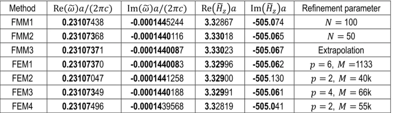
We have benchmarked several methods for computing the eigenfrequency and the normalized field of the QNM with the lowest frequency at 𝑘𝑥= 0.5𝜋/𝑎, red arrow in Fig. 2(b). Its magnetic-field modulus is shown in Fig. 2(d). The field is calculated at the center of the metallic inclusion and normalized according to Eq. (7). Table 2 summarizes the most accurate results obtained by each method.
To improve the numerical accuracy, the three FMM implementations increase the number of Fourier harmonics 2𝑁 + 1 retained in the computation. The four FEM implementations rely on different strategies. FEM1 increases the FE order 𝑝 from 1 to 6, whereas FEM2-4 increase the number 𝑀 of mesh elements for a fixed FE order. FEM2 and
FEM4 are based on a second order FE and FEM3 is using a fourth order. These results correspond to the data obtained with the highest number of Fourier harmonics, the largest FEM order or the finest mesh, except for FMM3, for which the data in Table 2 are obtained by an extrapolation of the convergence curve, see Section 4.4.
Method Re(𝜔̃)𝑎/(2𝜋𝑐) Im(𝜔̃)𝑎/(2𝜋𝑐) Re(𝐻̃𝑧)𝑎 Im(𝐻̃𝑧)𝑎 Refinement parameter
FMM1 0.23107438 -0.0001445244 3.32867 -505.074 𝑁 = 100 FMM2 0.23107368 -0.0001440116 3.33018 -505.065 𝑁 = 50 FMM3 0.23107371 -0.0001440087 3.33023 -505.067 Extrapolation FEM1 0.23107370 -0.0001440083 3.32996 -505.062 𝑝 = 6, 𝑀 =1133 FEM2 0.23107047 -0.0001441258 3.32900 -505.130 𝑝 = 2, 𝑀 = 40k FEM3 0.23107349 -0.0001440188 3.32991 -505.061 𝑝 = 4, 𝑀 = 66k FEM4 0.23107496 -0.0001439568 3.32819 -505.041 𝑝 = 2, 𝑀 = 55k
Table 2. Most accurate numerical values obtained for the complex eigenfrequency and the normalized magnetic field 𝐻̃𝑧𝑎. The last column summarizes the values of the refinement parameter used to obtain the data. Note that 𝐻̃𝑧𝑎 is not
a dimensionless quantity and is expressed in A. s. m−1/2. kg−1/2. For FMMs, 𝑁 represents the truncation rank, and
for FEMs, 𝑝 is the FE order and 𝑀 is the number of mesh elements. Bold digits (in the present Table and in following ones) are believed to be correct.
Figure 3 shows how the different numerical methods converge towards their best values. The convergence is displayed as a function of the CPU time (or wall time) in seconds. We have represented the relative difference between the data and a reference. For the reference, we chose the mean value of the results given by the three FMM1,2,3 that provide the largest number of common digits in Table 2. Figure 3 evidences that all seven methods converge towards the same values both for the eigenfrequency and for the normalized field. Remarkably, the real and imaginary parts of the eigenfrequency are obtained with at least six significant digits, see the bold numbers in Table 2. The real and imaginary parts of the field are obtained with two and four significant digits, respectively.
For this 2D problem, the wall times required to reach such an excellent accuracy span between a few seconds and one hundred for the slowest. The three FMM implementations converge faster than the FEM implementations. Note that the FEM is generally fast at extracting a large number of the eigenvalues spectrum at once, whereas the benchmark concerns a single eigenvalue. Note also that increasing the FEM order instead of refining the mesh leads to a faster convergence.
Figure 3. Convergence performance obtained for the QNM with the lowest frequency at 𝑘𝑥= 0.5𝜋/𝑎. Data are
displayed as a function of the CPU time in seconds. We present the relative difference between every calculation and a reference value obtained by averaging the results of FMM2, FMM3, and FEM1. (a) Real part of the eigenfrequency. (b) Imaginary part. (c) Real part of the normalized magnetic field. (d) Imaginary part. Black squares: FMM1. Magenta x-marks: FMM2. Green dots: FMM3. Red triangles: FEM1. Blue circles: FEM2. Brown pluses: FEM3. Cyan diamonds: FEM4.
3.2 Example 2: metal grating
3.2.1 General overview of the structure
The second benchmark considers an open structure: a 1D grating, made of a periodic slit array etched in a free-standing gold membrane, see Fig. 4(a). The geometry is based on [Col10]. The period is 𝑎 = 482.5 nm, the rod width 𝑤 = 347.5 nm and the rod height ℎ =130 nm. A Drude gold relative permittivity is considered, 𝜀𝑟(𝜔) = 1 − 𝜔𝑝2/(𝜔2+ 𝑖𝛾𝜔) with 𝜔𝑝= 1.15e16 𝑠−1 and 𝛾 = 0.0078 𝜔𝑝. This model agrees well with experimental ellipsometric data in the near infrared, but fails to describe the response of gold in the blue region of the spectrum.
The grating exhibits a valuable bandpass filtering behavior in transmission [Col10]. The specular transmission 𝑇0 and absorption A are shown in Figs. 4(b) and (c) for 3 in-plane wavevector 𝑘𝑥 values and for TM polarization (i.e. 𝐻𝑧 component parallel to the wires). The spectra are obtained using a collection of direct FE computations by iterating over the wavelength and the parallel momentum of the incoming plane wave [Dem07]. Note that in the frequency domain, handling the frequency dispersion of materials is trivial since the permittivity can be updated from tables as the frequency is swept. The goal of the second benchmark is to retrieve with accuracy the QNMs accounting for the main resonant transmission peaks in Figs. 4(b) and 4(c).
Figure 4 (a) Geometry of the free-standing 1D grating. (b) Specular transmission 𝑇0 for three values of 𝑘𝑥,
𝑘𝑥𝑎 𝜋⁄ = 0.05, 0.4,0.6. (c) Absorption 𝐴 (fraction of the incident energy absorbed) spectra. The dotted vertical
lines represent the Rayleigh anomalies. The dashed lines represent the real parts of the grating QNM eigenfrequencies 2𝜋𝑐/𝜔̃ taken from Fig. 5. The widths of the rectangular patches centered around each dashed line are set to be 2Im(2𝜋𝑐/𝜔̃), encoding the quality factor of each resonance. The inset is a zoom with the same color conventions, showing near normal incidence sharp resonances and the corresponding QNMs labelled C1 and D1 in Fig. 5.
3.2.2 Dispersion relation
The dispersion relation of the grating is shown in the right panel of Fig. 5. It has been computed using FEM4 (crosses) and a pole search method based on FMM3 (small dots forming a seemingly continuous line). The real parts of the normalized eigenvalues 𝜔̃/𝜂 with 𝜂 = 2𝜋𝑐/𝑎 are represented in ordinate. The abscissa represents the normalized Bloch wavevector in the first reduced Brillouin zone. The imaginary part of the normalized eigenvalues is encoded into a jet color scale of the dots and crosses that form the dispersion curves. For Re(𝜔̃)/𝜂 < 1.2, the dispersion relation exhibits six branches, labeled “A”, “B” … “F” and standing below the folded light line shown with dashed gray lines. The insets show the QNM fields |𝐇̃|.
Figure 5 Dispersion relation of the gold grating. Crosses represent the real parts of the eigenvalues obtained with
FEM4. Dots forming an almost continuous curve represent the real parts of the eigenvalues found using a complex pole search. The insets represent the modulus of the magnetic field distribution of the QNM corresponding to the eigenvalue indicated by a black line. The left panel shows a zoom close to the center of the Brillouin zone.
With the help of the dispersion curves, we may interpret the main features of the transmission and absorption spectra of Fig. 4(b)-(c). Let us begin with band B, for which Re(𝜔̃)/𝜂 lies between 0.493 and 0.83, corresponding to wavelengths in the interval [581; 979] nm. The QNMs can be directly linked to the absorption spectrum, when superimposing to the absorption peaks of Fig. 4(c) with rectangular patches centered at Re(2𝜋𝑐/𝜔̃) with widths 2Im(2𝜋𝑐/𝜔̃). In particular, the real parts shown with dashed vertical lines exactly match the maxima of the absorption spectrum for the three values of 𝑘𝑥.
Now, let us move to higher frequencies with the two high sharp absorption peaks (𝐴 ≈ 50%) observed for 𝑘𝑥 = 0.05𝜋/𝑑 and shown in the zoom Fig. 4(c). Again, when superimposing patches corresponding to 𝜔̃𝐷1 and 𝜔̃𝐶1, it appears again that these high peaks are attributable to the excitation of the QNMs D1 at 495 nm and C1 at 497 nm (see the zoom in the left panel in Fig. 5). Note that in the inset of Fig. 4(c), the central peak Re(2𝜋𝑐/𝜔̃𝐷1) is almost superimposed with the Rayleigh anomaly corresponding to the first diffraction order. This is consistent with the fact that band D meets the first folded light line for 𝑘𝑥≳ 0.05𝜋/𝑑 as it can be clearly seen on the zoom of the dispersion relation in Fig. 5. Theses QNMs cannot be excited at normal incidence for symmetry arguments and they cannot be excited either for large 𝑘𝑥 values since branches C and D both reach the folded light line for 𝑘𝑥≈ 0.05𝜋/𝑑.
In conclusion, all the resonant features of the absorption spectrum are understood from the dispersion relation. Note that, to recover all the features of the transmission spectra (not only the peaks, but also the zeros of 𝑇0 on the blue side of every peak), one needs to compute many QNMs [Gra18].
3.2.3 Numerical results for one selected eigenmode
The grating benchmark concerns the numerical computation of a single QNM (labelled B3 in Fig. 5) responsible for the absorption peak centered at 650 nm in Fig. 4(c). Two numerical values are benchmarked: The complex eigenfrequency 𝜔̃𝐵3𝑎/(2𝜋𝑐) and the normalized eigenfield at one point 𝐻̃𝑧,𝐵3(0, ℎ), the origin being chosen at the center of the rod and ℎ being the height of the rod. The results are shown in Table 3 and Fig. 6 for seven different numerical codes. The real and imaginary parts of the normalized eigenfield 𝑎𝐻̃𝑧,𝐵3 are shown in Fig. 6(e-f). The refinement parameter for each method is indicated in the right column. All methods show remarkable agreement, with at least four significant digits for the eigenvalue and three for the eigenfield.
parameter FMM1 0.74303−0.012662𝑖 101.358+761.312𝑖 𝑁 = 100 FMM2 0.7430756−0.0126𝑖 101.91+761.305𝑖 𝑁 = 50 FMM3 0.74307571−0.012660590𝑖 101.867+761.313𝑖 Extrapolationa FEM1 0.74307569−0.012660593𝑖 101.887+761.304𝑖 𝑝 = 6, 𝑀 = 1256 b FEM2 0.74305−0.0126644𝑖 101.99+761.93𝑖 𝑀 = 123k FEM3 0.74304−0.0126608𝑖 101.46+761.64𝑖 𝑀 = 67k FEM4 0.74310−0.0126553𝑖 101.89+760.79𝑖 𝑀 = 281k
Table 3. Most accurate numerical values obtained for the complex eigenfrequency 𝜔̃𝐵3𝑎/(2𝜋𝑐) and the normalized
magnetic field 𝐻̃𝑧,𝐵3(0, ℎ)𝑎. The refinement parameter for each method is indicated in the upper right column. a The convergence curve is calculated up to 𝑁 = 201 and extrapolated, see Section 4.4.
b Refinement by the element polynomial degree 𝑝, see Section 4.3.
As previously, we have represented in Fig. 6 the relative difference between the data and a reference. For the reference, we chose the mean value of the results given by FMM2,3, and FEM1. These methods are the ones that have the largest number of common digits, see Table 3. The conclusions regarding convergence are very similar to those made for the first benchmark. However, the convergence speed appears to depend significantly on the implementation, with some implementations of the FMM converging slower than the faster implementations of the FEM, see the convergence-rate results of Figs. 6(a)-(d). Among the FEM codes, FEM2-4 have the same refinement parameter, the number 𝑀 of mesh elements, whereas for the FEM1, the refinement parameters are the element polynomial orders 𝑝 (up to 𝑝 = 6) and of the mesh refinement around the corners that is predefined with a refinement length ℎ proportional to 10−𝑝/2.
Figure 6 – Convergence performance obtained for the QNM labelled B3 in Fig. 5 (second lowest eigenfrequency
for 𝑘𝑥= 0.4𝜋/𝑎). Data are displayed as a function of the CPU time. We present the relative difference between
every calculation and a reference value obtained by averaging the results of FMM2, FMM3, and FEM1. (a) and (b) Relative difference for real and imaginary parts of 𝜔̃𝐵3𝑎/(2𝜋𝑐). (c) and (d) Relative difference for real and
imaginary parts of 𝐻̃𝑧,𝐵3(0,h). The color convention is the same as in Fig. 3: Black squares: FMM1. Magenta
x-marks: FMM2. Green dots: FMM3. Red triangles: FEM1. Blue circles: FEM2. Brown pluses: FEM3. Cyan diamonds: FEM4. (e) and (f) Maps of the normalized QNM 𝐻̃𝑧,𝐵3.
3.3 Example 3: Nanocube antenna
The third benchmark is related to a 3D geometry, a nanocube antenna that belongs to the family of nanoresonators relying on slow gap-plasmons [Lal18a]. This geometry has recently attracted much attention for various applications and fundamental studies, from biochemical sensors, photodetectors, metamaterials, non-linear switches or light sources [Mor12,Aks14], to the test of spatial dispersion (non-locality) in metals [Cir12]. The geometry is directly inspired by the experimental work in [Aks14], see Fig. 7(a). A 8-nm-thick polymer spacer is sandwiched between two metals, a silver nanocube and a gold substrate. We use a bi-pole Drude model for silver and a quadruple-pole Drude-Lorentz model for gold, to accurately take into account the material dispersion, see details in the caption of Fig. 7(a).
Figure 7. Ag nanocube antenna of size 65 nm deposited on a 8-nm-thick polymer film (refractive index 1.5) coated
on an Au substrate. (a) Silver is modeled as a Drude metal, with 𝜆𝑝= 2𝜋𝑐 𝜔⁄ 𝑝= 138 nm and 𝛾 = 0.0023𝜔𝑝.
For gold, we use a Drude-Lorentz model, with 𝜔1= 1.317 × 10¹⁶ rad/s, 𝛾1= 6.216 × 10¹³ rad/s, 𝜔2=
4.572 × 10¹⁵ rad/s, and 𝛾
2= 1.332 × 10¹⁵ rad/s. The cube corners are rounded with a 4-nm radius. The left
panel shows the fine tetrahedral mesh used with FEM1, see Section 4.3. (b) The red point, located in the median plane of the polymer (𝑧 = 4 nm), shows the point 𝒓0 where the mode volume is computed. (c) Electric field
distribution of the fundamental magnetic-dipolar mode that resonates in the red. Owing to the symmetry, another QNM exists at the same complex eigenfrequency with a field distribution rotated by 90° around the 𝑧-axis. The distributions are computed with the FD method for a 1-nm discretization-grid.
The nanocube geometry offers deep-subwavelength field confinements and enhancements. In the visible spectral range, the response is governed by two dominant QNMs, the fundamental magnetic-dipole-like mode in the red spectrum and an electric-dipole mode in the green spectrum. Only the magnetic mode will be considered hereafter. Its resonance mechanism can be understood from a Fabry-Perot model with a slow gap-plasmon bouncing back and forth between gap extremities, and its resonance linewidth results from several contributions, photon radiation in air,
surface-plasmon launching around the nanocube, and metal absorption mainly around the nanogap in the metal. The respective impacts of each contribution on the QNM lifetime have been analyzed comprehensively in [Fag15].
We focus on two quantities related to the fundamental mode, the complex resonance wavelength 𝜆̃ and the complex mode volume 𝑉̃ of the magnetic-dipole-like mode for the benchmark. Figure 7b shows the precise position 𝒓0 of the 𝑧-polarized dipole source located in the median plane of the polymer film, which is used for the computation of 𝑉̃. Figure 7(c) displays the electric-field distribution of the magnetic-dipole mode. The fundamental mode is degenerate, meaning that there are two fields with the same eigenvalue due to the C4v symmetry of the configuration. Any linear combinations of these two modes are again eigenmodes, which renders the selected cases particularly interesting. Only one mode is shown in the Figure, the other mode being obtained by a 90° rotation around the 𝑧-axis. Table 4 summarizes the main results obtained for 𝜆̃ and 𝑉̃ by the five partners. The numbers correspond to the most accurate results obtained for “sampling grids” with the highest resolution. Concerning the resonance wavelength and setting aside the results obtained with FD-TU, an excellent agreement is obtained between the two other methods. Probably due to the rounded corners, the FD scheme suffers from inaccuracies compared to the two FEMs that provide nearly identical results. This explains the 15 nm shift-difference for Re(𝜆̃) between the second column and others. This shift is rather expected. Because of the tiny modal volume (𝑅𝑒(𝑉̃) ≈ 4 × 10⁻⁵𝜇𝑚3), it is inevitable that numerical inaccuracies such as those related to sampling result in large shifts of the resonance frequency (the nanocube is an excellent sensor in the real world, and thus a sensitive testcase for numerics). The five methods rely on the normalization of Eq. (6). They provide very similar mode volumes. Overall, we conclude that a good agreement is achieved; the peak deviations being < 2% for Re 𝜆̃, Im 𝜆̃ and Re 𝑉̃, and 2.4% for Im 𝑉̃.
We conclude that, even for a complicated 3D geometries made of two different metals, a very good accuracy (a few percent for 𝜆̃) which is often largely enough for analyzing experimental data can be reached with modest computational efforts (CPU time < 1 min), and this by all methods. We conclude that 3D QNM solvers are available on the shelves.
Methods 𝜆̃ [𝜇𝑚] 𝑉̃ [𝜇𝑚3] × 104 Refinement type
FD 0.6810+0.0159𝑖 0.392+0.030𝑖 1 nm mesh size FEM1 0.66585+0.015574𝑖 0.38449+0.02926𝑖 𝑝 = 4, 𝑀 = 40k
FEM2 0.66559+0.015362𝑖 0.386+0.0283𝑖 𝑝 = 1, 𝑀 = 276k
FEM3 0.66517+0.015468𝑖 0.384+0.0287𝑖 𝑝 = 2, 𝑀 = 220k
FEM4 0.66501+0.015395𝑖 - 𝑝 = 2, 𝑀 = 51k
Table 4. Nanocube with rounded corners.
Three partners have additionally performed the same computations by considering a perfectly cubic nanocube with sharp corners and edges. The results computed for the highest numerical resolution or extrapolated are show in Table 5. The mean value is λ̃ = 0.6996+0.143𝑖 with a standard deviation 0.0034+0.0004𝑖. A slightly larger deviation is obtained for 𝑉̃. Again the agreement is quantitative between all the methods.
Methods 𝜆̃ [𝜇𝑚] 𝑉̃ [𝜇𝑚3] × 10−4 Refinement type
FMM1 0.6974+0.01412𝑖 0.40987+0.02515𝑖 𝑁 = 55
FD 0.7053+0.0148𝑖 0.4217+0.0260𝑖 1 nm mesh size Table 5. Nanocube with 90° corners.
The benchmark geometry initially proposed was a 3D nanocube with rounded corners, see Fig. 7(a). For simplicity, we have also considered a nanocylinder geometry with exactly the same materials, the cube being just replaced by a silver cylinder with a 70-nm diameter and 65-nm height. For the mode volume, a 𝑧-polarized electric dipole placed at a distance 25√2 nm from the cylinder axis is considered. With the axisymmetry, the implementation is easier and more methods have been tested. In addition the computational results are more accurate than for the cube case, as shown by the data in Table 6.
Methods 𝜆̃ [𝜇𝑚] 𝑉̃ [𝜇𝑚3] × 10−4 Refinement type
FMM1 0.66369+0.01480𝑖 0. 645+0.0427𝑖 𝑁 = 50
FMM3 0.663557+0.0146866𝑖 0.63898+0.04616𝑖 𝑁 = 385 + extrapol. FEM1 0.66356+0.014687𝑖 0.6420+0.045631𝑖 𝑝 = 4, 𝑀 = 1086
FEM3 0.6644+0.01452𝑖 0.58+0.0400𝑖 𝑝 = 2, 𝑀 = 5k
FD 0.6753+0.0150𝑖 0.523+0.040𝑖 1 nm mesh size Table 6. 2D axisymmetry cylinder nanoantenna.
4. Method implementation and discussion
This Section provides details that each participant judge important for the readership. It does not include a full presentation of the methods, which have been published elsewhere. However we include all specific modifications made in order to improve the performance.
The FMM (also known as the RCWA) [Moh95,Lal96,Li98] relies on an analytical integration into one (longitudinal) direction of the space and on Fourier series expansions in the two (transversal) others. In the direction of integration, the system is sliced into several layers that have translational symmetry. Maxwell’s equations are transformed in each layer into an equivalent algebraic eigenvalue problem, whose eigenmodes propagate or decay within the layers. By using these eigenmodes as a basis for the expansion of an arbitrary field, no discretization is needed in the direction of translational symmetry, making the FMM rather efficient for a restricted numbers of layers. Due to the use of Fourier expansions in the transversal directions, the FMM is restricted to periodic geometries. By incorporating absorbing boundaries or PMLs in the transverse directions, the FMM can be also used for non-periodic structures as well [Sil01]. It is known as the aFMM (“a” for “aperiodic”). The accuracy of the FMM or the aFMM increases with the truncation rank 𝑁 of the Fourier series, corresponding to a total number of retained Fourier harmonics of (2𝑁 + 1 ) in 2D or (2𝑁 + 1 )2 in 3D.
The FEM and FD methods are also well established methods that are used in many fields. The interested reader may refer to the textbook [Jin02] for a review in electromagnetism. Both methods rely on a full discretization of space and the accuracy increases with the number of unknowns that is proportional to the number 𝑀 of mesh elements and increases with the order 𝑝 of the FE scheme used.
4.1 LP2N, Bordeaux
GB RAM and an Intel(R) Xeon(TM) CPU X5660 @ 2.80GHz processor.
The first freeware, QNMEig, has been launched in 2018. It includes a QNM-solver [Yan18] to compute and normalize QNMs and PML-modes and, in a second step, to reconstruct the field scattered by the micro and nanoresonators in the QNM basis. In general, accurate reconstructions are obtained with tens or hundreds of QNMs retained in the expansion, depending of the geometry, see details in [Yan18].
QNMEig relies on the eigenfrequency solver of the electromagnetic radio frequency (RF)/optics module of COMSOL Multiphysics [Comsol]. The COMSOL solver computes a large number (set by the user) of QNMs only for non-dispersive media and does not normalize the field. For dispersive media, it approximately transforms nonlinear eigenvalue problems to linear ones by performing second-order Taylor expansion of complex material parameters with respect to some frequency set by user, the so-called linearization point. Thus, such approximate approach cannot accurately find modes away from the linearization point.
QNMEig is in fact an extension of the COMSOL solver that accurately handles dispersive media by coupling the build-in (RF)/optics module and the weak-form module, so that it can be very easily operated by COMSOL users. It relies on the auxiliary-field formulation, see Section 2.4 and [Yan18]. QNMEig normalize the modes by computing the volume integral of Eq. (6). It has been used for the three benchmarks. The CPU-time for solving 3D problems such as the present nanocube antenna of Example 3 or a photonic crystal cavity [Cog18], is typically 2 min with a standard desktop computer, see more details in [Yan18]. Two minutes are in general enough to get accurate results for the QNM field and eigenvalue, to challenge experimental data. QNMEig and the companion MATLAB Tooboxes are available at the group webpage [http]. The package includes the four COMSOL model sheets of the benchmarked geometries, the plasmonic crystal, the grating and the nanocube and nanocylinder antennas, and also one tutorial example, a metal sphere in air, for which a document, presenting step by step details on how starting a QNMEig simulation, is offered from the perspective of new users.
The second freeware, QNMPole, is based on the pole-search algorithm described in [Bai13]. It calculates and normalizes the modes of plasmonic or photonic micro/nanoresonators by successive iterations, starting from an initial guess value. The pole-search approach is completely general and can be used with arbitrary geometries and materials, and with a large variety of frequency-domain Maxwell’s equations solvers. It has been tested for instance with FMM1, FMM3, FMM2 and FEM3, and could have been used with the other methods as well. For researchers that use COMSOL Multiphysics as a standard Maxwell equation solver operating at real frequencies (electromagnetic RF and optics modules), QNMPole includes a few MATLAB programs that operate under MATLAB-COMSOL livelink and allow the user to compute and normalize QNMs, and customize their specific demands with MATLAB programming. The use of QNMPole is recommended if one just needs to compute a few modes, or if the permittivity of some constitutive materials cannot be cast into a N-pole Lorentz-Drude model (required for QNMEig), or if the material is not reciprocal.
When QNMPole and QNMEig are both used with the same mesh, they provide exactly the same eigenfrequencies and normalized fields. The coincidence has been checked for each benchmark, and for many other examples. This is why only one set of data is shown for the LP2N results. In addition to the QNM-solver, QNMPole and QNMEig also include pedagogical MATLAB toolboxes to reconstruct the scattered field in the QNM bases, to calculate the absorption/extinction cross-sections or the Purcell factor. Finally note the QNMs computed for the grating case are eigenvectors with a complex 𝜔̃ for a fixed in-plane real wavevector 𝑘𝑥, implying that the QNMs are the pole that would be revealed in experiments by varying the frequency of the incident beam, while maintaining for each frequency the product 𝜔 sin 𝜃 constant. This implies that the angle of incidence 𝜃 be tuned between every spectrum measurement. In reality, however, 𝜃 is usually fixed during the acquisition of the spectrum data. Thus, considering the
exact experimental protocol, further investigations into QNM computation and normalization for fixed 𝜃 shall be investigated [Gra18].
4.2 TU-Delft
The reduced-order modal solver FD used to determine QNMs in arbitrarily-shaped dispersive 3D structures on open domains is based on a Lanczos-type reduction method that exploits a particular symmetry property of Maxwell's equations. The approach consists in casting the Maxwell equations and the second-order dispersive relations into first-order form using auxiliary field variables and discretize the resulting system in space. Outgoing wave propagation is taken into account via a particular realization of the perfectly matched layer technique in which complex spatial step sizes match the layer PML to the computational domain on a subset of the complex-frequency plane [Dru16,Dru13]. The order of the resulting discretized first-order system is typically very large (millions of unknowns in 3D) so that a direct computation of the QNMs is usually not feasible. Fortunately, the system is symmetric with respect to the discrete counterpart of the bilinear form of Eq. (6) [Lal18] and allows us to efficiently compute the QNMs via a three-term Lanczos-type recursion relation. Only three vectors defined on the total computational domain need to fit into the computational memory due to this three-term relation. Finally, the scattered field of the resonator can be efficiently reconstructed as well without any significant additional computational costs [Zi16a,Zi16b].
The FD solver uses finite-differences to come to a symmetrizable dynamic system which depends nonlinearly on the frequency because of either the dispersive PML used or the dispersion of the material. We stress that FD solver can be used for other types of discretizations that are symmetrizable. In practice, we use a linearized PML that is matched to the frequencies of QNMs of interest, to get rid of the nonlinearity introduced by the PML. Using auxiliary fields, we then obtain a linear shifted system that is symmetric in the bilinear form. The QNMs can then efficiently be computed as the Lanzos-Ritz pairs of this system using short term recurrence relations [Zi16a,Zi16b]. The current implementation of the FD solver relies on a MATLAB prototype implementation with a simple gridding routine for the geometries.
For the 3D nanoantenna geometry, we use second-order finite-differences and consider seven different discretization meshes to study the convergence performance of the FD solver for the geometry with sharp corners and edges with a MATLAB 2016 implementation run on 4 of the 14 cores of a single Intel Xeon E5-2695 v3 CPU at 2.30GHz. The accuracy of the computational results increases quadratically as the discretization step decreases. The computation time behaves linear with the number of degrees of freedom, which themselves increase cubically with the discretization step. Thus, the error expressed in computation time approximately scales as O(time-2/3).
Currently the FD method relies on a simple gridding algorithm with straightforward medium averaging to obtain the finite-difference system. Compared to the FEMs, meshing of complex geometries with round corners and edges with finite-difference methods is challenging. We experienced some difficulties while gridding the rounded corners of the nanocube benchmark and therefore only computed the QNMs for the two finest meshes, and our values deviate by approximately 2% from the FEM results in Table 6. Although the error made remains reasonably low for a nanoresonator that is ultrasensitive to fabrication or numerical imperfections, this motivates us to further develop the solver by using more advanced homogenization and averaging schemes to better capture the geometry in the future.
Due to the Lanczos algorithm, 99% of the wall time of the FD-TU method is spent on sparse matrix-vector and vector-vector products. This shows the potential of the method for GPU implementations to obtain faster runtimes. Concerning memory requirements, our algorithm needs to store three double precision complex vectors of the size of the number of degrees of freedom. For a 2-nm discretization, this means that 579 MB of storage is required. In the
current implementation the runtime of our algorithm is roughly 1/6000 s/#core/#degree-of-freedom as the runtime scales close to linear with the number of degrees of freedom.
4.3 Zuse Institute Berlin
FEM1 relies on the FEM software package JCMsuite, which is developed by JCMwave at ZIB and which is also commercially available. JCMsuite includes solvers for time-harmonic Maxwell eigenvalue [Zsc06] and scattering [Pom07]problems, as well as for further problem classes. The implementation includes higher-order finite elements, with ℎ- and 𝑝-adaptivity, mesh generators for tetrahedral, prismatoidal and mixed meshes, and adaptive PMLs, which allows to handle also resonance problems with structured exterior domains [Ma13].
For benchmarks 1 and 2, we have used the resonance mode solver included in JCMsuite which solves the nonlinear eigenvalue problem using an auxiliary field approach. For computing QNMs with increasing resolution, we use a MATLAB script which defines the physical and numerical project parameters, invokes the solver for QNM computation and for post-processing. In a loop, numerical accuracy is increased stepwise by increasing the polynomial order 𝑝 of the used finite elements, 𝑝 = 1 …6, and by simultaneously increasing the mesh resolution at the metal corners. The initial guesses for the eigenfrequency is chosen as 2𝜋𝑐𝜔𝑎 = 0.231 (Benchmark 1) and 2𝜋𝑐𝜔𝑎 = (0.74−0.013𝑖) (Benchmark 2). In each step of the loop, the guess is updated with the prior result. Computation of the normalized field values is performed by computing solutions with Bloch vectors 𝑘𝑥 and 𝑘−𝑥 and applying Eq. (7). Figure 8(a)-(b) shows the relative error of the real and imaginary parts of 𝜔̃ and 𝑉̃. Here, the relative error δA of quantity A is defined as deviation from a quasi-exact solution AQE, i.e., δA = |𝐴 − AQE|/|AQE| . As quasi-exact solution for the eigenfrequency and normalized field, we use results obtained with the highest numerical accuracy setting, 𝑝 = 6.The relative errors are displayed as function of number of unknowns of the discrete problem which increases with increased finite element degree 𝑝 and with increased mesh resolution.
For benchmark 3, we have used a recently developed contour integral method based on Riesz projections [Zsc18]. We solve scattering problems along a complex contour around the eigenfrequency of interest instead of solving the nonlinear eigenproblem directly. The resulting Riesz projection is normalized within a post-process.
We increase the numerical resolution by increasing the finite element degree up to p=5. Figures 8(c)-(d) show the relative error (see above) of 𝜔̃ and 𝑉̃ for the nanocube and nanocylinder. The relative errors are plotted over the number of unknowns for the scattering solver. We choose three integration points for the contour integration, i.e., three scattering problems are solved for a given finite element degree 𝑝. The quasi-exact solution is the numerical result obtained with 𝑝 = 5. The unstructured mesh for the nanocube is shown in Fig. 7(a), it contains 40522 tetrahedrons with a minimal edge length of about 0.06 nm and a maximal edge length of about 36 nm. The fine meshing around the rounded corners and edges of the nanocube ensures that the geometry model error is sufficiently small. We have checked that further refinement of the corners changes the numerical results at 𝑝 = 4 (most accurate results in the plots in Fig. 8) only by amounts smaller than the obtained accuracy. E.g., the impact of further refining the mesh on Re (𝜔̃) is below 10−5. At a numerical resolution with 𝑝 = 4 we obtain a resonance wavelength of 𝜆̃= 665.8529 + 15.57386𝑖 nm ± 0.0184 + 0.00092𝑖 nm. At a numerical resolution with 𝑝 = 5 we obtain a resonance wavelength of 𝜆̃= 665.8510 + 15.57396𝑖 nm.
For the nanocylinder, we consider a two-dimensional cross section of a rotationally symmetric geometry. The unstructured mesh consists of 1086 triangles. At a numerical resolution with 𝑝 = 4 we obtain a resonance wavelength of 𝜆̃= 663.5622 + 14.68720𝑖 nm ± 0.0207 + 0.00197𝑖 nm. At a numerical resolution with 𝑝 = 5 we obtain