HAL Id: hal-02371337
https://hal.archives-ouvertes.fr/hal-02371337
Submitted on 19 Nov 2019
HAL is a multi-disciplinary open access
archive for the deposit and dissemination of
sci-entific research documents, whether they are
pub-lished or not. The documents may come from
teaching and research institutions in France or
abroad, or from public or private research centers.
L’archive ouverte pluridisciplinaire HAL, est
destinée au dépôt et à la diffusion de documents
scientifiques de niveau recherche, publiés ou non,
émanant des établissements d’enseignement et de
recherche français ou étrangers, des laboratoires
publics ou privés.
Ewelina Rupnik, Marc Deseilligny
To cite this version:
Ewelina Rupnik, Marc Deseilligny. More surface detail with One-Two-Pixel Matching. [Research
Report] IGN - Laboratoire MATIS. 2019. �hal-02371337�
More surface detail with
One-Two-Pixel Matching
Ewelina Rupnik, Marc Pierrot Deseilligny
Abstract—Photogrammetrically derived Digital Surface Mod-els have been widely adopted in geoscientific applications such as mapping and change detection across volcanic surfaces, glaciers, areas of seismic activity, forests, river landforms etc. Resolution of the reconstructed surface is crucial as more accurate information enables more profound understanding of the phenomena. With this objective in mind, the research presented here proposes a new matching cost function that produces surfaces of enhanced resolution with respect to the gold standard: the window-based semi-global matching technique. We evaluate the algorithm on different image datasets spanning various acquisition geometries, radiometric qualities and ground sample distance sizes. In par-ticular, results on Earth satellites (SPOT-7, Pl´eiades), extraterres-trial (Chang’E3 moon landing), aerial and terresextraterres-trial acquisitions are shown. The implementation of the method is available in MicMac – the free open-source software for photogrammetry.
I. INTRODUCTION
Digital surface model (DSM or photogrammetric DSM) gen-eration using dense image matching is an accepted technique across the geoscience communities. Next to other competitive techniques such as LiDAR or radar, image-based reconstruction produces denser 3D information, it is cost-effective and richer as it includes photometric observations that allow, for example, 3D change detection or classification. Photogrammetric DSMs in geoscience applications can be generated from terrestrial images, unmanned aerial vehicle (UAV) acquisitions or high-resolution optical satellite imaging.
a) Terrestrial and UAV applications: Modelling of sur-face roughness parameters [1]; mapping volcanic sursur-faces [2]; and measuring glaciers’ microrelief progression [3] are some of many examples of terrestrial applications carried out with consumer grade cameras and little expert knowl-edge. UAV-based surveys are increasingly presented as an alternative to terrestrial surveys due to their larger reach, their ease of deployment and reduced operational cost. With respect to resolution, UAV surveys are a compromise between high-resolution close-range and moderate-resolution satellite imaging. The success of the UAV technology is reflected in numerous publications which show that UAV-collected imagery can: enable modelling of forest canopy height [4]; determine the rate and extent of landslide movements [5]; quantify coastal erosion [6], [7] and deposition processes [8] in aeolian research; map ultrafine (i.e. centimetric) tectonic faults in tectonic research [9]; or be employed in repeated surveys of the ice-sheet masses in glaciology [10].
b) Earth satellite and extraterrestrial applications: With the available optical satellite data provided by modern (e.g. Pl´eiades 1A/B, SPOT-satellites, QuickBird, WorldView 2/3/4, CubeSat) or older satellites (e.g. CartoSat, ASTER), we can
capture the Earth’s surface at ground sampling distances (GSD) in the range of 0.3 metres to some metres, yielding DSMs of a similar resolution [11]. Coupled with daily revisit times, satellite images are a suitable tool for mapping the surface evolution. To take a few state-of-the-art examples, satellite images are used to: identify patterns and rates of sand dune migrations [12]; quantify seismic surface displacement [13], [14]; estimate timber volume in a densely forested area [15]; study the time-varying coastal shelf [16]; employ multi-temporal DSMs for elevation change studies across glaciers, volcanoes and river landforms [17]; or map other planets’ topographies [18].
In all of the mentioned applications, the resolution of the surface plays a significant role because it improves the observability of the phenomena. Following the principle that one can more easily spot a small change if one can see more detail, an image matching algorithm that furnishes better resolution surfaces allows possible change detection at finer detail. Put simply, techniques that enable finer resolution could allow earlier change detection. The research presented in this publication addresses fine resolution surface reconstruction by proposing a novel image matching technique.
A. Related work
a) Generalities: Photogrammetrically derived DSMs are typically found by solving an energy function with global, semi-global matching (SGM) or local methods.
Classically, local methods calculate the best correspon-dences in three steps: (i) calculate matching cost, (ii) aggregate cost over a support domain, and (iii) select the depth by the Winner-Takes-All [19] or the belief propagation [20], [21] schemes. The local character of the methods makes them computationally efficient, often at the expense of lower 3D precision and completeness.
Whether through a global or SGM approach, the best correspondences are found by minimizing a cost function that is the sum of the data and the regularity term. Global methods minimize the energy defined over all pixels in a MRF graph with techniques such as α-expansion moves [22], [23] or message passing [24]. Alternatively, definition over a continuous space and sub-pixelar reconstruction precision is possible with variational methods [25]. Such minimization is NP-hard, and does not allow for concave regularity terms. The first poses memory issues for large scale reconstructions, while the latter inhibits faithful reconstruction at discontinuities (e.g. buildings).
The SGM methods are solved with multi-directional dy-namic programming techniques, impose no constraint on the
regularity term and the optimization is resolved along indepen-dent lines of pixels [26], [27]. Therefore, the computational times remain reasonable as the image size grows. Since cost function is cumulative along a number of directions, the found optimal solution is close to the global solution.
b) Matching cost calculation: Independent of the algo-rithm, many different measures exist that describe the simi-larity (i.e. photo-consistency) between pixel correspondences. The very first and most straightforward measure compares the pixel intensity values [28], [29]. However, pixel intensity difference are unreliable for matching in real-world conditions (i.e. non-Lambertian surfaces or, radiometric differences due to illumination change) and in the presence of non-textured zones or repetitive patterns. In practice, photo-consistency measures, e.g. zero-mean normalized cross-correlation (NCC), Census, Rank [30], Mutual Information [31], are defined over a support domain (square windows ordinarily of 3x3, 5x5, etc. size) [32]. Including more context within the per-pixel matching is advantageous because it increases the uniqueness and the robustness of the matched points, as well as attenuates the noise caused by the low signal-to-noise ratio of the sensor. Note, however, that (i) it interpolates the image signal within the support and possibly misses the surface fine structures, as well as (ii) a pixel-wise cost aggregated over a support window assumes constant disparity within the aggregated neighbour-hood. The latter results in smoothness artefacts or mismatches if it happens to overlap a discontinuity, e.g. a building’s edge. Furthermore, if the support window is chosen to be a square region, it takes for granted that the square shape in one view will project to an exact square in another view. Therefore, this technique neglects the perspective transformations the shape undergoes once projected to 3D and subsequently back-projected to another view (the so-called window foreshortening problem).
Numerous approaches have been proposed to overcome the above shortcomings. To mitigate the mismatches at discontinuities, adaptive support windows avoiding discontinuities [33], adaptive windows minimising a cost, or intensity gradient cost aggregation [27] were proposed. Sweeping-planes [34], 3D slanted windows [20], or a fusion of slanted and adaptive windows (i.e. elongated windows with different orientations) [35] were adopted to account for different surface slopes. Initialisation of the surface planes is carried out by analysing the sparse reconstruction [34], dense reconstruction computed with square windows [33] or by random assignment [20]. Each option carries some risk of missing the correct surface slope or providing incomplete initialisation. For instance, sparse reconstruction can initialize only in places where 3D points exist, hence omits poorly textured areas; classical dense reconstruction may fail to provide good initial surfaces at discontinuities and slopes; and random selection gives no guarantee of assigning the suitable plane slope to either of the pixels belonging to a region underlying that plane.
B. Contributions
In this work we aim to develop enhanced precision depth reconstruction free from fronto-parallel artefacts and with good performance at surface discontinuities. To realise this goal we:
– formulate a new matching cost defined over a single pixel, – adopt a second pixel to add context and allow for slope testing with minimum information (a slope is defined by two points in 3D space and it is tested with exactly two pixels),
– embed the image dense matching in a semi-global match-ing framework which favours slope coherence in the neighbourhood of a point and ensures surface continuity in poorly textured areas.
To increase the robustness of the reconstruction, the matching cost is defined in a multi-view constraint.
II. METHODS
A. One-Two-Pixel cost function
With the objective of excelling the spatial resolution of re-constructed depths, we propose a reformulated energy function (1): C(D) = N X p=1 CI(p, dp)+ X q=N p CC(dp, dq) + X q=N p CT(dp, dq) (1)
where CI is the single-pixel term, CC is the two-pixel term, CT is the smoothing term, N is the number of all
pixels, dpis a disparity at position p and dq is the disparity at
position q belonging to the Np neighbourhood of p. C(D) is
the minimum cost of assigning the optimal depths D across all pixels. The minimum solution is found in the following three steps: cost assignment (see Alg. 1), cost aggregation (see Alg. 2) and the optimal depth selection. The described methods are implemented in MicMac – the free open-source software for photogrammetry [36].
a) Two-pixel data term: CC encodes the dissimilarity of
a two-pixel window across multiple views (N bV ), see Eq. (2). Ideally, the advantages of the minimum window are twofold: (i) it is more apt to reconstruct fine 3D scene structure than the usual square correlation window, and (ii) it is less susceptible to noisy data than as if only the single pixel term was used.
Employing the CC is equivalent to iterating over d q and
verifying the coherency of a given slope with the image data, the final cost of a slope assignment being an accumulation of the dissimilarities calculated independently for each stereo pair. Speaking in terms of the cost structure, the CC costs can be associated with arcs (in analogy to CT), rather than with nodes as is the case of CI (see Alg. 2 and Fig. 1). Note that the two-pixel term should not be confused with the smoothness term. The latter applies ”blind” penalization, without considering the pixel intensity values.
For a depth assignment dp, the CC cost will depend on
the differences of normalised intensity ratios at position p and q. The choice of ratios was made to guarantee a robust comparison in the presence of additive and multiplicative illumination changes across the views. The role of P dsC is
to control the relative influence of the CC term in the cost
function. In all of our tests, it was also set to 1.0.
CC(dp, dq) = P dsC· 1 N bV − 1· N bV X v=1 Iv dp I0 dp −I v dq I0 dq (2)
b) Single-pixel data term: CI is the cost of assigning a particular depth to the position p. It is implemented as a truly one-pixel measure and conveys the dissimilarity of two pixels in multiple views (N bV ), see Eq. (3). To match the dynamic range of the two-pixel term, it is expressed as a mean of all (1− intensity ratios) between the master I0and the secondary
Iv. The δv parameter is added to model the view-dependent
radiometric differences that may disturb the cumulative cost (this is unlike in the CC expression where the effect of the
radiometry change is fully modelled by the difference of ratios). The value of the parameter is a function of intensity ratios between the master image and a secondary image. It can be pixel-dependent – if non-constant radiometric corrections across the images are necessary (e.g. specular reflections) – or take a global value per image pair (i.e. master and secondary image couple; see Alg. 1 where δv is computed on a pixel
basis). When a pixel-dependent case is chosen, the ratios shall be first smoothed by simple averaging or by 2D polynomial function fit.
P dsI is a weighting factor and it plays the same role as
P dsC. In all of our tests, we set the value to 1.0.
c) Regularizing term: The standard regularization func-tion present in MicMac library has been adopted and it is not discussed hereafter (see [26] and [37] for more details on the subject). CI(p, dp) = P dsI· 1 N bV − 1· N bV X v=1 " 1 − I v dp δv· Id0p # (3) III. RESULTS A. Datasets
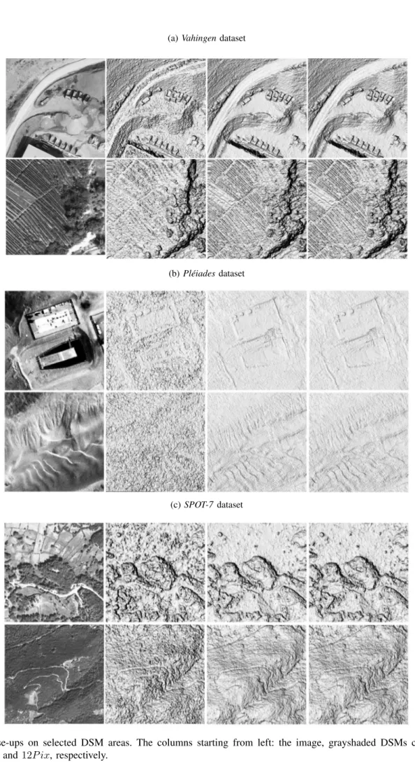
a) Aerial acquistion – Vaihingen dataset: A set of four aerial images acquired with the UltraCam-X camera at 0.2m GSD is used in this experiment. The images are part of the EuroSDR Matching benchmark [38]. The camera calibration and orientation parameters were also furnished with the bench-mark. The available ground truth (GT) data is a surface that is a median of several DSMs furnished by all of the participants of the benchmark. As a result, many surface details are discarded and the GT is considered unsuitable to evaluate the One-Two-Pixel matching algorithm. The evaluation was carried out on an alternative GT (cf. Section III-B) over an area of ≈ 5km x 3km (cf. Fig. 7a and Fig. 8a).
Figure 1: Top: One-Two-Pixel cost structure corresponding to a stereo pair. In grey is the surface to be inferred from the matching. Cp,dpI and Cq,dqI are the costs of taking disparity dp at p and dq at q , respectively. Cdp,dpC is the cost of assigning a given slope. Bottom: A stereo pair that feeds the cost structure. The cost structure is illustrated on a stereo pair in epipolar geometry, however, the implemented algorithm is not constrained by the number of views and, by default, operates in the original image geometry.
b) Satellite acquisition I – Pl´eiades dataset: This scene was acquired by a tri-stereo pair from the Pl´eiades 1B satellite. It is entirely covered by sand dunes of varying patterns, situ-ated in northern Chile. As a preliminary processing step, the satellite orientation parameters were refined in a RPC-bundle adjustment using methods described in [39]. The evaluation was carried out on an alternative GT (cf. Section III-B) over an area of ≈ 7.5km x 5.5km (cf. Fig. 7b and Fig. 8b).
c) Satellite acquisition II – Spot-7 dataset: A Spot-7 tri-stereo pair is used in this experiment. The scene represents a rural zone with rich vegetation and varying altitudes. Refined satellite orientation parameters in the form of a replacement grid were furnished with the dataset. Evaluation is carried out within a ≈ 2km x 2km region (cf. Fig. 7c and Fig. 9) on a GT described in Section III-B.
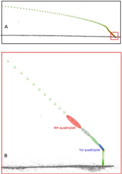
d) Extra-terrestrial acquisition – Chang’E 3 dataset: In late 2013, the People’s Republic of China launched a lunar surface exploration mission known as Chang’E 3. To calculate the explorer’s trajectory (cf. Fig. 2), over 150 conic images acquired at landing were downloaded1 and post-processed using Structure-from-Motion methods in MicMac. The images were available in a heavily compressed jpeg format.
Reference data in the form of a 1.5m orthophoto and a 30m resolution DSM produced from the Lunar Reconnaissance
Algorithm 1 Cost assignment
V Im[v].ImOrth(X, Y ) - intensity in image v at position (X, Y ); all images are orthorectified to the geometry of the master
ratio(int, int) - calculate ratios norm(int) - normalise to [-127,127] δ - radiometric calibration
Surf Opt - optimiser
. Assignment for Z = Zmin; Z < Zmax; Z + + do
for X = 0; X < Sz.x; X + + do for Y = 0; Y < Sz.y; Y + + do V0= V Im[0].ImOrth(X, Y ) CI = 0 for v = 0; v < N bV ; v + + do Vk= V Im[v].ImOrth(X, Y ) V al = ratio(V0, Vk) V al = norm(V al) r.push back(V al)
Vcor k = δvVk V alcor= ratio(V 0, Vkcor) CI+ = Abs(V alcor) end for
. Communicate the vector of ratios and the data term to the optimiser Surf Opt(X, Y, Z) = r Surf Opt(X, Y, Z) = CI end for end for end for
Orbiter Camera2 (LROC) images served to geo-reference the images. The provided reference data is of much lower resolution then the produced DSMs (i.e. 0.25m). Because of this, an alternative GT was created and is detailed in the following Section III-B.
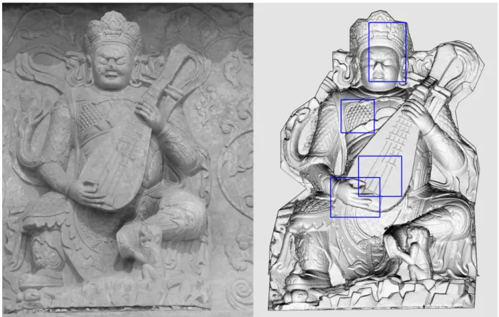
e) Terrestrial acquisition: The last dataset is a sequence of 5 images taken with a long focal length DSLR camera (i.e., f = 105mm), see Fig. IV. It does not undergo quantitative evaluation but is shown to demonstrate the performance of the One-Two-Pixel matching on large discontinuities (cf. Figs. 12 and 13).
B. Ground truth creation
Due to the lack of GT availability, we adopted a strategy where full resolution images serve to establish the GT surfaces, and are compared against surfaces calculated using lower resolution images. Following this concept, the GTs of the Vaihingen/ Pl´eiades / Spot-7 datasets are denoted with the Z1
2http://lroc.sese.asu.edu
Figure 2: Chang’E 3 explorer moon landing trajectory. (A) ≈ 150 images acquired before the landing. (B) Close-up of the end trajectory, the highlighted sets of images correspond to images used in the processing. The surface calculated with the 4thquadruplet is compared against a surface produced by
a fusion of all the quadruplets.
postfix corresponding to zoom 1, or the full resolution images. Analogously, the Z2 postfix signifies zoom 2, or half the full resolution images. In other words, the matching GSDs are as follows: GSDV aihingenZ1 = 0.2m, GSDV aihingenZ2 = 0.4m, GSDP leiades
Z1 = 0.5m, GSDP leiadesZ2 = 1.0m, GSD Spot−7
Z1 =
1.5m, and GSDZ2Spot−7= 3.0m. As there is no obvious choice
as to which reconstruction method to employ to create the GT, two sets of GTs are adopted: a GT calculated with cross-correlation similarity measure (CORRZ1) and a GT obtained
with the One-Two-Pixel measure (12P ixZ1).
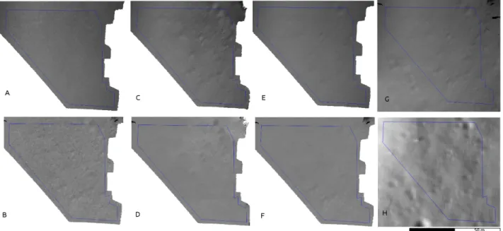
Because the Chang’E 3 dataset features a large number of images of varying scales, we have chosen to calculate the GT based on the images obtained with larger scales (i.e. those takes closer to the planet surface). Using this GT, we then evaluate surfaces obtained from images taken at higher altitudes. Nonetheless, the footprints of the images closer to the surface are smaller, and consequently, cover a smaller area than the surface under evaluation. To match the surface extent and further enhance the quality of the GT, we perform surface reconstruction from multiple sets of quadruplets, and subsequently fuse them in 3D as presented in [11]. In Fig. 2, the evaluated image set (i.e., 4th quadruplet) is highlighted in red, while the gray-green-blue sets (i.e., 1st–3rd q.) are used to produce the GT. All surfaces were re-sampled to a 0.25m grid which corresponded to the mean GSD of 4thquadruplet. See also Fig. 10 (G)-(H) for the output GT surface and the LROC orthophoto, respectively.
Algorithm 2 Cost aggregation
for each direction + do . forward
for each direction - do . backward
for X = 0; X < Sz.x; X + + do for Y = 0; Y < Sz.y; Y + + do
for DZ = Zmin; DZ < Zmax; DZ + + do
Cost = CostOf DZ(DZ) . get the value of concave cost function at DZ rk = Surf Opt.rOf k(k) . recover the vectors of ratios
rk+1= Surf Opt.rOf k(k + 1)
. calculate the two-pixel cost and add to cost Cost+ = T woP ixCost(rk, rk+1)
. communicate the two-pixel cost to the optimiser Surf Opt.U pdateCostOneArc(rk+1, Dir, Cost)
end for end for end for end for end for C. Evaluation strategy
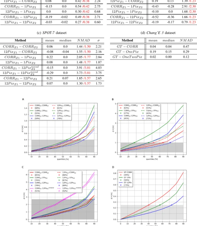
The results are interpreted in terms of accuracy measures suited to (i) normal distribution observations (i.e., mean, median, standard deviation) calculated on DSMs’ signed dif-ferences ∆h, as well as (ii) non-normal errors, insensitive to outliers and calculated on absolute differences |∆h| (i.e. Normalised Mean Absolute Deviation (NMAD) and sample quantiles) [40]. Sample quantiles enable us to infer the per-centage of errors that fall within a specified interval. The statistics are presented in Tab. I and Fig. 4.
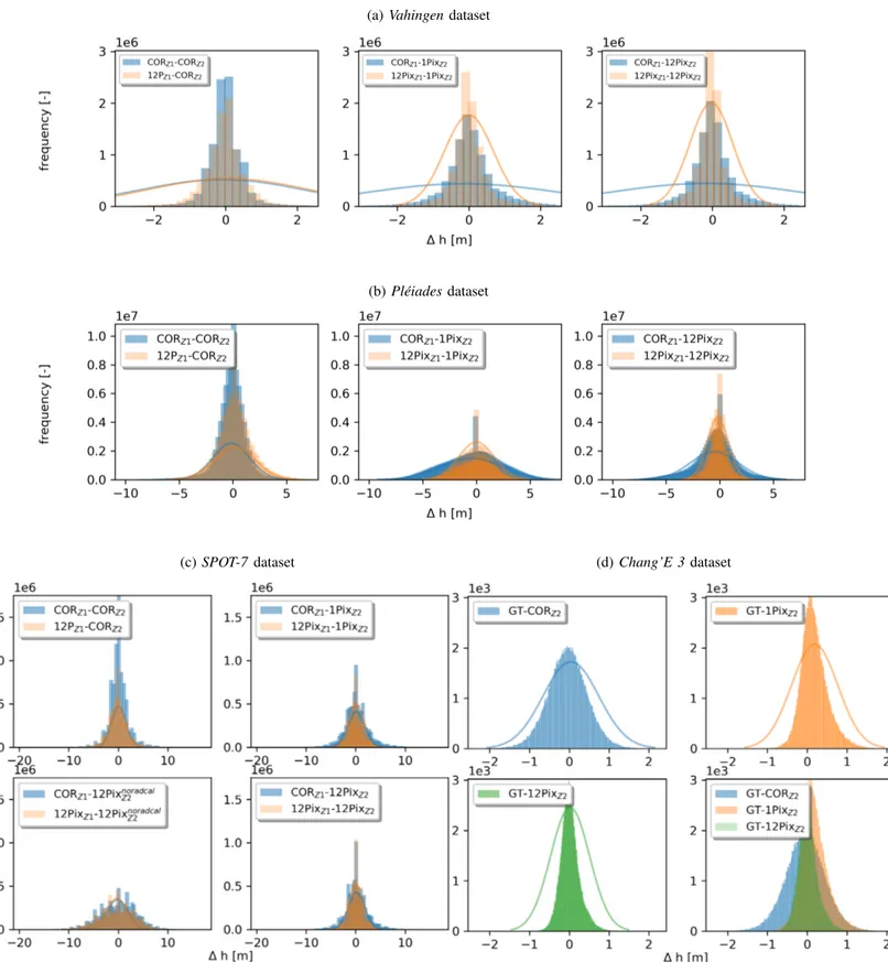
Additionally, theoretical histograms and histograms of ∆h are plotted in Fig. 5. In Fig. 6 height profiles are drawn, and in Figs. 7, 8, 9, 10, qualitative results in the form of gray-shaded DSMs are given.
D. Discussion
a) Aerial acquistion – Vaihingen dataset: Where the CORRZ1was considered the GT, all ∆h manifest a
system-atic shift of the DSM and a strongly non-normal distribution (compare the mean with the median and the σ and N M AD in Tab. Ia). Further evidence of the non-normality of the distribution is the mismatch between the theoretical histogram and the histogram calculated on the data, as is shown in Fig. 5a. The ≈ 2m standard deviations are probably due to the fact that the CORRZ2 DSM is incapable of discerning
the small vegetation rows which make up a lot of the area of interest. Furthermore, note the fidelity with which the 12P ixZ2 and 1P ixZ2 reconstruct at discontinuities, and in
flat, non-textured zones (cf. Figs. 6a, 7a and 8a).
According to the sample quantiles, there is a tendency for DSMs compared to 12P ixZ1 (cf. dashed lines in Fig. 4)
to perform better than those compared to CORRZ1. The
three best sample quantiles corresponding to the size of the
GSD are 76%, 71%, and 68% for 12P ixZ1 − 12P ixZ2,
12P ixZ1− 1P ixZ2and CORRZ1− CORRZ2, respectively.
In other words, 76%, 71%, and 68% of errors will be found within the interval of h0, GSDi.
b) Satellite acquisition I – Pl´eiades dataset: The dataset’s quantitative error metrics and the qualitative inter-pretation of the results are incoherent. The lowest mean and medianscores are observed for 12P ixZ1− 1P ixZ2, followed
by CORRZ1−CORRZ2and CORRZ1−12P ixZ2. However,
the standard deviations and N M AD follow the inverse order: the performance of 12P ixZ1 − 12P ixZ2 precedes that of
CORRZ1− CORRZ2 (cf. Fig. Ib). This could be partially
explained by the increased level of noise observed in the images. While 12P ix and CORR can attenuate the noise due to their support regions and the cost function smoothing term, the 1P ix has only the latter. However, this does not necessarily mean that more detailed surfaces are reconstructed with either – observe the surface details reconstructed with 12P ix and 1P ix yet invisible to CORR in Figs. 6b, 7b and 8b. This puts in question the chosen GT and the error metric used.
The spread between the N M ADs and the standard devia-tions signals, as previously, a non-normal error distribution.
c) Satellite acquisition II – Spot-7 dataset: The speci-ficity of the images is the changing illumination across the triplet pair (cf. Fig. 3 for image intensity ratios). To demon-strate the efficacy of the radiometric calibration proposed in the algorithm, the 12P ixZ2DSM is calculated twice: with and
without the calibration. Calibration using a global value per image pair turned sufficient to model the illumination effect. Note in Tab. Ic the significant improvement in accuracy with the correction applied.
The ∆h in all cases match the normal distribution errors relatively well (cf. Fig. 5c; except the non-calibrated result). The 12P ixZ2performs best of all (cf. Tab. Ic) and obtains the
lowest N M AD and σ measures, while its mean and medium scores are placed ex aequo with CORRZ2. All surfaces but
the CORRZ2exhibit a systematic shift when compared to the
CORRZ1 GT.
According to the sample quantile curves, when the CORRZ1 is considered GT, 85% of CORRZ2, 76% of
1P ixZ2 and 78% of 12P ixZ2 DSMs’ errors lay within the
h0, GSDi interval. When the 12P ixZ1 was used, the
pro-portions of DSMs’ errors are: 84% for CORRZ2, 87% for
1P ixZ2, and 89% for 12P ixZ2 DSMs.
d) Extra-terrestrial acquisition – Chang’E 3 dataset: 1P ix DSM comprises a systematic error revealed by the mean and median measures, while in contrast CORR and 12P ix DSMs reveal correspondingly insignificant or no bias (cf. Tab. Id). This behaviour can be explained by the fact that 1P ix cost function, defined on a single pixel, becomes too ambiguous to find the correct surface. On the other hand, CORR and 12P ix cost functions include more context therefore remain close to the true surface. Until now, this behaviour has not been observed, nonetheless, the quality of the images in other datasets was incomparably better and free from compression artefacts. Notice the different character of noise here and in Satellite acquisition I, having per pixel structure and arranged in blocks, respectively.
40% of the CORR DSM, 56% of the 1P ix DSM and 73% of the 12P ix DSM errors lay within the interval of h0, GSDi (cf. Fig. 4). The long tails of the theoretical histogram distri-bution in 12P ix and 1P ix DSMs suggest that some outliers are present in the data (cf. Fig. 5d). Irrespective of that, the 12P ix DSM is the unquestionable winner among other results for this dataset. The height profiles drawn over craters and on flat ground in Fig. 6d and the DSMs shown in Fig. 10 confirm the high fidelity of 12P ix DSM.
The evaluation is carried out within a region of interest marked in blue in Fig. 10.
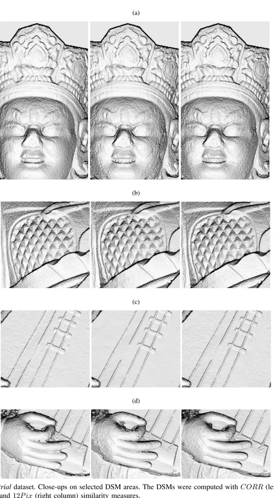
e) Terrestrial acquisition: Finally, in Fig. 13 several areas of interest of the reconstructed statue are shown. The evaluation metrics are (i) performance on slopes and (ii) the level of surface detail. The results are: the CORR surfaces are smoother than the 1P ix and 12P ix; the 1P ix produces artefacts at large slopes; the 12P ix performs best in terms of the level of detail and at discontinuities. In particular, note the following points of interest:
• in Fig. 13a, the band over the forehead and the cheek
close to the ear;
• in Fig. 13b, the repetitive pyramid pattern and upper left
image corner for directional matching artefacts;
• in Fig. 13c, the cords of the guitar as well as the level of
noise on the flat area; and
• in Fig. 13d, the separation of fingers, as well as the parts of the guitar.
IV. CONCLUSION
We have presented a new matching cost function that is embedded in a semi-global matching framework. The method was tested on 5 different datasets (1 aerial, 2 satellite, 1 extra-terrestrial and 1 extra-terrestrial dataset), 4 of which were evaluated
qualitatively and quantitatively. The quantitative assessment is twofold: based on comparing DSMs’ reconstructions calcu-lated with different similarity measures (i.e. cross-correlation, one-pixel and one-two-pixel); and by comparing to reference surfaces of higher resolution. During evaluation, normal and non-normal error distribution metrics are taken into account, as well as histograms, surface profiles and gray shaded surfaces. The normal surface metrics do not reveal a clear winner among all methods and suggest their inappropriateness for our experiments. The distribution-free error metrics (i.e., N M AD and sample quantiles) unanimously point to our method as the better performer. In all experiments the 12P ix sample quantile curves report the best measurement accuracies.
Similarly, the visual assessment of the surface quality indicates that both the 12P ix and the 1P ix DSMs convey more detail than the correlation-based DSMs. The 12P ix and 1P ix exhibit similar performance except in two cases: when considerable flaws in image quality are present and for large slopes. In these two cases, the 12P ix similarity measure outperforms the 1P ix.
ACKNOWLEDGMENT
We would like to thank Renaud Binet from CNES for providing us with the Chang’E 3 dataset, Tristan Faure and Antoine Levenant from IGN for giving us access to Spot7 im-ages and Arthur Delorme from IPGP for the Pl´eiades imim-ages.
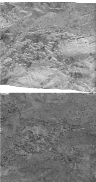
Figure 3: SPOT-7 dataset. Ratios of intensities between the master image and two secondary images. The images are ortho-rectified to the geometry of the master image. If the ratios had similar values, the radiometric correction would be superfluous.
Table I: Mean, median and standard deviation scores calculated on DSMs signed differences, |∆h|. Three GT DSMs are present in the table: CORRZ1 computed with cross-correlation, 12P ixZ1 with One-Two-Pixel measures and GT computed
as a fusion of multiple quadriplets. The values in read are mean N M AD scores computed on all available GTs. The values are expressed in meters.
(a) Vahingen dataset
Method mean median N M AD σ CORRZ1− CORRZ2 -0.08 -0.02 0.34/0.38 2.32 12P ixZ1− CORRZ2 0.08 0.0 0.42/0.38 2.24 CORRZ1− 1P ixZ2 -0.15 0.0 0.54/0.42 2.75 12P ixZ1− 1P ixZ2 0.0 0.0 0.30/0.42 0.68 CORRZ1− 12P ixZ2 -0.19 -0.02 0.49/0.38 2.71 12P ixZ1− 12P ixZ2 -0.03 -0.02 0.27/0.38 0.60 (b) Pl´eiades dataset
Method mean median N M AD σ CORRZ1− CORRZ2 -0.14 -0.06 1.06/1.23 1.76 12P ixZ1− CORRZ2 0.19 0.13 1.39/1.23 1.96 CORRZ1− 1P ixZ2 -0.43 -0.28 2.91/2.30 2.91 12P ixZ1− 1P ixZ2 -0.10 0.0 1.68/2.30 1.65 CORRZ1− 12P ixZ2 -0.52 -0.36 1.66/1.23 2.22 12P ixZ1− 12P ixZ2 -0.19 -0.17 0.79/1.23 1.00 (c) SPOT-7 dataset
Method mean median N M AD σ CORRZ1− CORRZ2 0.06 0.0 1.44/1.50 2.21 12P ixZ1− CORRZ2 -0.08 -0.04 1.55/1.50 2.16 CORRZ1− 1P ixZ2 0.22 0.0 2.05/1.77 2.84 12P ixZ1− 1P ixZ2 0.08 0.0 1.48/1.77 1.87 CORRZ1− 12P ixnocalZ2 -0.15 0.0 3.91/3.81 4.03 12P ixZ1− 12P ixnocalZ2 -0.29 0.0 3.73/3.81 3.75 CORRZ1− 12P ixZ2 0.21 0.07 1.85/1.57 2.65 12P ixZ1− 12P ixZ2 0.07 0.0 1.30/1.57 1.73 (d) Chang’E 3 dataset
Method mean median N M AD σ GT − CORR 0.04 0.04 0.47 0.49 GT − OneP ix 0.19 0.15 0.29 0.34 GT − OneT woP ix 0.02 0.00 0.12 0.24
Figure 4: Sample quantiles calculted on: A. Vahingen, B. Pleiades, C. Spot-7, D. Chang’E 3 datasets. The gray zone indicates |∆h| values that are ≤ GSD (of the lower resolution images). The × markers correspond to sample quantiles for respective GSD values, i.e., they signal the percent of all ∆h for which h0 ≥ |∆h| ≤ GSDi.
(a) Vahingen dataset
(b) Pl´eiades dataset
(c) SPOT-7 dataset (d) Chang’E 3 dataset
Figure 5: ∆h histograms calculated for all datasets and Ground Truths (i.e., CORRZ1, 12P ixZ1 and GT ). Superimposed
(a) V ahing en dataset (b) Pl ´eiades dataset (c) SPO T -7 dataset (d) Chang’E 3 dataset Figure 6: Height profiles dra wn o v er DSMs computed with C O R RZ 1 (in red), 1 P ix Z 1 (in blue) and 12 P ix Z 1 (in green).
(a) Vahingen dataset
(b) Pl´eiades dataset
(c) SPOT-7 dataset
Figure 7: Close-ups on selected DSM areas. The columns starting from left: the image, grayshaded DSMs computed with CORR, 1P ix and 12P ix, respectively.
(a) Vahingen dataset.
(b) Pl´eiades dataset.
Figure 8: Grayshaded representation of surfaces reconstructed with different methods and at different resolutions. A. CORRZ2,
Figure 9: Spot-7 dataset. Grayshaded representation of surfaces reconstructed with different methods and at different resolutions. A. CORRZ2, B. 12P ixnoRadCalZ2 , C. 1P ixZ2, D. 12P ixZ2, E. CORRZ1, F. 12P ixZ1.
Figure 10: Chang’E 3 dataset. Surfaces reconstructed with (A) COR, (C) 1P ix, (E) 12P ix similarity measures, as well as (G) the GT surface. The surface differences ∆h for (B) GT − COR, (D) GT − 1P ix, (F) GT − 12P ix. (H) is the LROC orthophoto and in blue is the region of interest.
(a)
(b)
(c)
(d)
Figure 13: Terrestrial dataset. Close-ups on selected DSM areas. The DSMs were computed with CORR (left column), 1P ix (middle column) and 12P ix (right column) similarity measures.
REFERENCES
[1] F. Bretar, M. Arab-Sedze, J. Champion, M. Pierrot-Deseilligny, E. Heggy, and S. Jacquemoud, “An advanced photogrammetric method to measure surface roughness: Application to volcanic terrains in the piton de la fournaise, reunion island,” Remote Sensing of Environment, vol. 135, pp. 1–11, 2013.
[2] S. Kolzenburg, M. Favalli, A. Fornaciai, I. Isola, A. Harris, L. Nan-nipieri, and D. Giordano, “Rapid updating and improvement of airborne lidar dems through ground-based sfm 3-d modeling of volcanic features,” IEEE Transactions on Geoscience and Remote Sensing, vol. 54, no. 11, pp. 6687–6699, 2016.
[3] A. K¨a¨ab, L. M. R. Girod, and I. T. Berthling, “Surface kinematics of periglacial sorted circles using structure-from-motion technology,” 2014. [4] J. Lisein, M. Pierrot-Deseilligny, S. Bonnet, and P. Lejeune, “A pho-togrammetric workflow for the creation of a forest canopy height model from small unmanned aerial system imagery,” Forests, vol. 4, no. 4, pp. 922–944, 2013.
[5] U. Niethammer, S. Rothmund, M. James, J. Travelletti, and M. Joswig, “Uav-based remote sensing of landslides,” International Archives of Photogrammetry, Remote Sensing and Spatial Information Sciences, vol. 38, no. Part 5, pp. 496–501, 2010.
[6] S. d’Oleire Oltmanns, I. Marzolff, K. D. Peter, and J. B. Ries, “Un-manned aerial vehicle (uav) for monitoring soil erosion in morocco,” Remote Sensing, vol. 4, no. 11, pp. 3390–3416, 2012.
[7] M. James and S. Robson, “Straightforward reconstruction of 3d surfaces and topography with a camera: Accuracy and geoscience application,” Journal of Geophysical Research: Earth Surface, vol. 117, no. F3, 2012. [8] C. H. Hugenholtz, K. Whitehead, O. W. Brown, T. E. Barchyn, B. J. Moorman, A. LeClair, K. Riddell, and T. Hamilton, “Geomorphological mapping with a small unmanned aircraft system (suas): Feature detection and accuracy assessment of a photogrammetrically-derived digital terrain model,” Geomorphology, vol. 194, pp. 16–24, 2013.
[9] K. Johnson, E. Nissen, S. Saripalli, J. R. Arrowsmith, P. McGarey, K. Scharer, P. Williams, and K. Blisniuk, “Rapid mapping of ultrafine fault zone topography with structure from motion,” Geosphere, vol. 10, no. 5, pp. 969–986, 2014.
[10] J. C. Ryan, A. L. Hubbard, J. E. Box, J. Todd, P. Christoffersen, J. R. Carr, T. O. Holt, and N. A. Snooke, “Uav photogrammetry and structure from motion to assess calving dynamics at store glacier, a large outlet draining the greenland ice sheet,” 2015.
[11] E. Rupnik, M. Pierrot-Deseilligny, and A. Delorme, “3D reconstruction from multi-view VHR-satellite images in MicMac,” ISPRS Journal of Photogrammetry and Remote Sensing, vol. 139, pp. 201–211, 2018. [12] E. Hermas, S. Leprince, and I. A. El-Magd, “Retrieving sand dune
movements using sub-pixel correlation of multi-temporal optical remote sensing imagery, northwest sinai peninsula, egypt,” Remote sensing of environment, vol. 121, pp. 51–60, 2012.
[13] A. Rosu, M. Pierrot-Deseilligny, A. Delorme, R. Binet, and Y. Klinger, “Measurement of ground displacement from optical satellite image correlation using the free open-source software micmac,” ISPRS Journal of Photogrammetry and Remote Sensing, vol. 100, pp. 48–59, 2015. [14] A. Vallage, Y. Klinger, R. Grandin, H. Bhat, and M. Pierrot-Deseilligny,
“Inelastic surface deformation during the 2013 Mw 7.7 Balochistan, Pakistan, earthquake,” Geology, vol. 43, no. 12, pp. 1079–1082, 2015. [15] C. Straub, J. Tian, R. Seitz, and P. Reinartz, “Assessment of cartosat-1
and worldview-2 stereo imagery in combination with a lidar-dtm for timber volume estimation in a highly structured forest in germany,” Forestry, vol. 86, no. 4, pp. 463–473, 2013.
[16] K.-H. Tseng, C.-Y. Kuo, T.-H. Lin, Z.-C. Huang, Y.-C. Lin, W.-H. Liao, and C.-F. Chen, “Reconstruction of time-varying tidal flat topography using optical remote sensing imageries,” ISPRS Journal of Photogrammetry and Remote Sensing, vol. 131, pp. 92–103, 2017. [17] L. Girod, C. Nuth, A. K¨a¨ab, R. McNabb, and O. Galland, “Mmaster:
Improved aster dems for elevation change monitoring,” Remote Sensing, vol. 9, no. 7, p. 704, 2017.
[18] K. Gwinner, F. Scholten, F. Preusker, S. Elgner, T. Roatsch, M. Spiegel, R. Schmidt, J. Oberst, R. Jaumann, and C. Heipke, “Topography of mars from global mapping by hrsc high-resolution digital terrain models and orthoimages: characteristics and performance,” Earth and Planetary Science Letters, vol. 294, no. 3-4, pp. 506–519, 2010.
[19] K.-J. Yoon and I.-S. Kweon, “Locally adaptive support-weight approach for visual correspondence search,” in Computer Vision and Pattern Recognition, 2005. CVPR 2005. IEEE Computer Society Conference on, vol. 2. IEEE, 2005, pp. 924–931.
[20] M. Bleyer, C. Rhemann, and C. Rother, “Patchmatch stereo-stereo matching with slanted support windows.” in Bmvc, vol. 11, 2011, pp. 1–11.
[21] S. Galliani, K. Lasinger, and K. Schindler, “Massively parallel multiview stereopsis by surface normal diffusion,” in Proceedings of the IEEE International Conference on Computer Vision, 2015, pp. 873–881. [22] Y. Boykov, O. Veksler, and R. Zabih, “Fast approximate energy
min-imization via graph cuts,” IEEE Transactions on pattern analysis and machine intelligence, vol. 23, no. 11, pp. 1222–1239, 2001.
[23] T. Taniai, Y. Matsushita, Y. Sato, and T. Naemura, “Continuous 3d label stereo matching using local expansion moves,” IEEE Transactions on Pattern Analysis and Machine Intelligence, 2017.
[24] P. F. Felzenszwalb and D. P. Huttenlocher, “Efficient belief propagation for early vision,” International journal of computer vision, vol. 70, no. 1, pp. 41–54, 2006.
[25] R. Ranftl, S. Gehrig, T. Pock, and H. Bischof, “Pushing the limits of stereo using variational stereo estimation,” in Intelligent Vehicles Symposium (IV), 2012 IEEE. IEEE, 2012, pp. 401–407.
[26] M. Pierrot-Deseilligny and N. Paparoditis, “A multiresolution and optimization-based image matching approach: An application to surface reconstruction from spot5-hrs stereo imagery.” in ISPRS Workshop On Topographic Mapping From Space, vol. 36(1), Ankara, Turkey, February 2006.
[27] H. Hirschm¨uller, “Stereo processing by semiglobal matching and mutual information,” Pattern Analysis and Machine Intelligence, IEEE Trans-actions on, vol. 30, no. 2, pp. 328–341, 2008.
[28] T. Kanade, a. K. S. Kano, H., A. Yoshida, and K. Oda, “Development of a video-rate stereo machine,” in Intelligent Robots and Systems 95.’Human Robot Interaction and Cooperative Robots’, Proceedings. 1995 IEEE/RSJ International Conference on, vol. 3. IEEE, 1995, pp. 95–100.
[29] S. Birchfield and C. Tomasi, “A pixel dissimilarity measure that is insensitive to image sampling,” IEEE Transactions on Pattern Analysis and Machine Intelligence, vol. 20, no. 4, pp. 401–406, 1998. [30] R. Zabih and J. Woodfill, “Non-parametric local transforms for
comput-ing visual correspondence,” in European conference on computer vision. Springer, 1994, pp. 151–158.
[31] P. Viola and W. M. Wells III, “Alignment by maximization of mutual information,” International journal of computer vision, vol. 24, no. 2, pp. 137–154, 1997.
[32] Y. Furukawa and C. Hern´andez, “Multi-view stereo: A tutorial,” Foun-dations and Trends in Computer Graphics and Vision, vol. 9, no. 1-2,R
pp. 1–148, 2015.
[33] K.-J. Yoon and I. S. Kweon, “Adaptive support-weight approach for correspondence search,” IEEE Transactions on Pattern Analysis and Machine Intelligence, vol. 28, no. 4, pp. 650–656, 2006.
[34] D. Gallup, J.-M. Frahm, P. Mordohai, Q. Yang, and M. Pollefeys, “Real-time plane-sweeping stereo with multiple sweeping directions,” in Computer Vision and Pattern Recognition, 2007. CVPR’07. IEEE Conference on. IEEE, 2007, pp. 1–8.
[35] A. Buades and G. Facciolo, “Reliable multiscale and multiwindow stereo matching,” SIAM Journal on Imaging Sciences, vol. 8, no. 2, pp. 888– 915, 2015.
[36] E. Rupnik, M. Daakir, and M. Pierrot Deseilligny, “MicMac–a free, open-source solution for photogrammetry,” Open Geospatial Data, Soft-ware and Standards, vol. 2, no. 1, p. 14, 2017.
[37] M. Pierrot-Deseilligny, E. Rupnik, L. Girod, J. Belvaux, G. Maillet, M. Deveau, and G. Choqueux, “Micmac, apero, pastis and other bever-ages in a nutshell,” 2016.
[38] N. Haala, “Dense image matching final report,” EuroSDR Publication Series, Official Publication, vol. 64, pp. 115–145, 2014.
[39] E. Rupnik, M. Pierrot-Deseilligny, A. Delorme, and Y. Klinger, “Refined satellite image orientation in the free open-source photogrammetric tools Apero/MicMac,” ISPRS Annals of the Photogrammetry, Remote Sensing and Spatial Information Sciences, 2016.
[40] J. H¨ohle and M. H¨ohle, “Accuracy assessment of digital elevation models by means of robust statistical methods,” ISPRS Journal of Photogrammetry and Remote Sensing, vol. 64, no. 4, pp. 398–406, 2009.