HAL Id: hal-01323792
https://hal.archives-ouvertes.fr/hal-01323792
Submitted on 31 May 2016
HAL is a multi-disciplinary open access
archive for the deposit and dissemination of
sci-entific research documents, whether they are
pub-lished or not. The documents may come from
teaching and research institutions in France or
abroad, or from public or private research centers.
L’archive ouverte pluridisciplinaire HAL, est
destinée au dépôt et à la diffusion de documents
scientifiques de niveau recherche, publiés ou non,
émanant des établissements d’enseignement et de
recherche français ou étrangers, des laboratoires
publics ou privés.
A HMM Classifier with Contextual Observability:
Application to Indoor People Tracking
Adrian Bourgaud, François Charpillet
To cite this version:
Adrian Bourgaud, François Charpillet. A HMM Classifier with Contextual Observability: Application
to Indoor People Tracking. [Research Report] LORIA - Université de Lorraine. 2016. �hal-01323792�
A HMM Classifier with Contextual Observability:
Application to Indoor People Tracking.
Adrian Bourgaud
1, François Charpillet
1Abstract— Indoor tracking people activities with sensors networks is of high importance in number of domains, such as ambient assisted living. Home sensors have seen strong develop-ment over the last few years, especially due to the emergence of Internet of Things. A wide range of sensors are today available to be installed at home : video cameras, RGB-D Kinect, binary proximity sensors, thermometers, accelerometers, etc.
An important issue in deploying sensors is to make them work in a common reference frame (extrinsic calibration issue), in order to jointly exploit the data they retrieve. Determining the perception areas that are covered by each sensor is also an issue that is not so easy to solve in practice.
In this paper we address both calibration and coverage isssues within in a common framework, based on Hidden Mar-kov Models (HMMs) and clustering techniques. The proposed solution requires a map of the environment, as well as the ground truth of a tracked moving object/person, which are both provided by an external system (e.g. a robot that performs telemetric mapping).
The objective of the paper is twofold. On one hand, we propose an extended framework of the classical HMM in order to (a) handle contextual observations and (b) solve general classification problems. In the other, we demonstrate the relevancy of the approach by tracking a person with 4 Kinects in an apartment. A sensing floor allows the implicit calibration and mapping during an initial learning phase.
I. INTRODUCTION
People tracking is strategic in domains such as surveillance and domotics. Possible applications include monitoring of sensitive areas, and the development of activity recognition, since activities are often strongly correlated to specific areas [17]. Activity recognition for domotics aims at fall-detection of elderly people [5], monitoring of disabled people [9], and simplifying everyday living by anticipating people’ needs.
In the last few years, there has been a growing interest in multi-sensor fusion [11], which consists in the joint usage of several sensors (potentially of different nature). Using several sensors provides either additional information, or redundant information which increases the robustness of the system. People tracking is feasible through the use of a variety of sensors, including cameras [2], wearable objects [9], binary proximity sensors [6] and sensing ground [1].
Most fusion techniques are derived from probabilistic frameworks : Kalman Filter (KF), Extended KF (EKF), Unscented KF (UKF), as well as particle filters, are widely used for people tracking. Hidden Markov Models (HMMs) 1 A. Bourgaud and F. Charpillet are with Inria,
Villers-lès-Nancy, F-54600, France; CNRS, Loria, UMR n.7503 and Université de Lorraine, Loria, UMR n.7503,
Vandoeuvre-lès-Nancy, F-54500, France. [email protected]
franç[email protected]
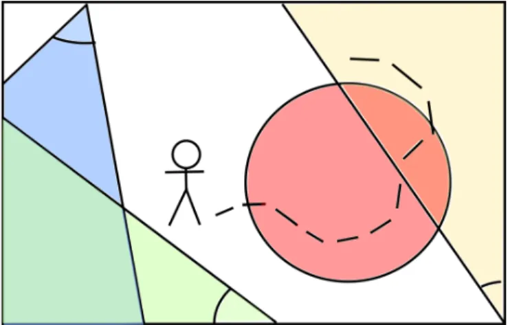
Fig. 1: A possible scenario. A person is moving in a room with three cameras (triangles) and a binary proximity sensor (circle).
could be used as well : even though the positions possibly occupied by a tracked person are reduced to a finite set, this model allows to take into consideration position-dependent observability that is not handled by the aforementioned filters, as we show in this paper.
The problem we address in this paper (depicted by Fi-gure 1) is to track a single person in an indoor environment with several (possibly multimodal) sensors, without making any assumption about the placement of these sensors. The proposed solution is based on HMMs, and similarly to HMM-based map-matching techniques [14, 10], the data re-trieved by the sensors is mapped to areas of the environment. The initialisation phase of the proposed solution requires a map of the environment, as well as the ground truth (real position of the person tracked), which are both provided by an external system (e.g. a robot that performs telemetric mapping). This external system is not needed thereafter. Our approach could be applied to calibrate systems with a more costly one that is temporarily available (e.g. rented).
The contribution of this paper is twofold : 1) Theoretical contributions :
a) A novel method to perform sequential classification with HMMs, that allows the number of classes to be different from the number of hidden states. b) A novel method to exploit contextual observability
in the multi-sensor case. It is possible to assess the perception areas of sensors in an unsupervised fa-shion by exploring the environment, and to exploit these constraints to improve tracking.
2) A proof of concept that the extrinsic calibration of sensors can be performed in an implicit manner in indoor environment.
The experiments on tracking a person presented in this paper validate these contributions. The sensor set used for tracking consists in 4 RGB-D cameras. The external system used for the initialisation is a sensing ground [1], but in the future we envision to use a mobile robot with localisation skills.
The remainder of this paper is structured as follows. In section II, related work is described. In section III, a short introduction to HMMs is provided, and a derived model for multi-sensor people tracking is presented as a first proposal. In section IV, a method to exploit contextual observability is addressed as a second proposal. In section V, the previous contributions are instantiated to the tracking of a person in an apartment with non-calibrated cameras. In section VI, experimental results are presented and analysed. Finally, conclusion and further works are proposed in section VII.
II. RELATEDWORK
Sensor calibration - While the literature is very dense concerning the explicit extrinsic calibration of sensors, very few techniques have been proposed to calibrate the sensors in an implicit manner, i.e. by finding correlations between their respective data. Advantages of implicit calibration methods regarding to explicit ones include the applicability to every type of sensors, and not making assumptions avout the placement of the sensors : the overlapping of their perception areas is not mandatory.
In [4, 15], the topology of the overall system is modeled by the travel times between the areas monitored by the cameras instead of a common map. It is suited for outdoor surveillance where it is not possible to use a map in the general case. However this travel times topology caries less information than a map.
In [7], the proposed system recognises patterns of dimen-sionality (space × time) from raw images of four cameras. The system is successful in finding common patterns when the fields of view of the cameras are overlapping. However this system is not transposable to people tracking due to the fact that it exploits low level features.
Contextual observability - In the literature, two types of missing data are opposed : Missing At Random (MAR) data, and Missing Not At Random (MNAR) data. The distribution of MAR data is uniform over the data, whereas the distribution of MNAR data is correlated to variables of the model. In the surveillance case, missing observations from sensors are MNAR because they are correlated to the perception areas of the sensors and hence, to the actual position of the person tracked.
The literature in people-tracking is sparse about the usage of MNAR observations. In [3], the quality as well as the theoretical fields of view of the sensors are taken into account in the probability pD of detecting a person in a given area,
but these informations are manually fed to the system. In [8], the informations retrieved by the sensors are weighted
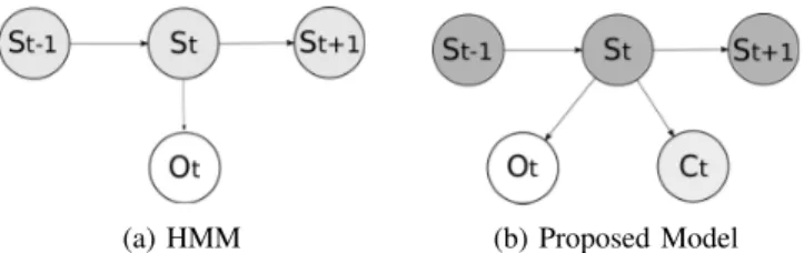
(a) HMM (b) Proposed Model Fig. 2: Graphical models. St is the hidden state, Ot the
corresponding observation, and Ctthe associated class. Light
grey : variables that are accessible solely during the learning phase. Dark grey : variables that are never accessible.
regarding to their a-priori observability, but this approach is not tractable when the placement of the sensors is a-priori unknown in indoor environments, as walls may constrain the perception areas of the sensors.
III. SEQUENTIAL CLASSIFICATION WITHHMMS
A. A short introduction to HMMs
HMM is a model that allows supervised learning of sequential information. An HMM is modeled by the tuple λ =< S, O, p(Stk|St−1,k0), p(S0k), p(Ot|Stk) > where S is a set of K hidden states S1, ..., SK, O is a set of T
sequential observations O1, ..., OT, p(Stk|St−1,k0) stands for the probabilities of transition between hidden states Sk0 and Sk from time t − 1 to t (follows a categorical distribution).
p(S0k) stands for the prior probability that the underlying
hidden state is Sk at time t = 0 (it follows a
categori-cal distribution). p(Ot|Stk) is the probability of observing
observation Ot given hidden state Stk, which is commonly
assumed to follow either a categorical distribution (discrete case) or a gaussian distribution (continuous case). Figure 2a shows an HMM as a graphical model.
The Expectation-Maximisation algorithm [19] allows to learn the parameters λ of the model. Its description may be found in [16, chapter 13]
Thereafter, the notation γ(Stk) will be used as a shorthand
for probability p(Stk|Ot, St−1,k0), which is computed for inference.
The classic way to train a HMM in a supervised manner is to force each hidden state to represent a class by feeding its probability p(Ot|Stk) with the observations expected for
that class. Even though it is also possible to train a HMM in an unsupervised manner by not forcing hidden states to represent anything specific and letting the system converge, by doing so the topology of the system is lost : it is impossible to assess what does each state represent. B. Proposed model
The goal of the model we introduce is to reach a com-promise between the awareness of the topology provided by the supervised method and the automated clustering of the unsupervised method. The model we introduce differs from an HMM in the sense that the set C of classes is distinct from the set S of hidden states.
This model (presented in Figure 2b) is described by λ =< S, O, C, p(Stk|St−1,k0), p(S0k), p(Ot|Stk), p(Ctj|Stk) >, where C is the set of classes and p(Ctj|Stk) is the probability
to be in class Ctj while in hidden state Stk.
The immediate consequence of manipulating distinct sets is that the number K of hidden states may differ from the number J of classes. When K = J, it is straightforward that this system performs as well as a classic supervised HMM, provided that each hidden state is paired to a class. When K < J, S may be seen as a clustering of C. This clustering is done in an unsupervised manner and is based on the likelihood that similar classes are correlated to similar observations. The hidden states from S are abstract clusters (as they merge both information from observations O and classes C), and probability p(Ctj|Stk) is the projection to
apply once Stk is inferred in order to head back to the
interpretable domain of classes C.
Learning is performed using the standard EM algorithm. During inference, we are willing to find the following probability : p(Ctj|Ot, St−1,k0) = K P k=1 p(Ctj|Ot, Stk, St−1,k0)p(Stk|Ot, St−1,k0) = K P k=1 p(Ctj|Stk)p(Stk|Ot, St−1,k0) = K P k=1 p(Ctj|Stk)γ(Stk) (1)
The case of K > J is not addressed in this paper. IV. MISSINGDATA
In this section we address to model MNAR observations that are correlated to the classes. As we exploit the model introduced in subsection III-B, by the play of conditional independencies, it is equivalent to address the problem of MNAR observations that are correlated to hidden states.
In [18], the authors tackle the problem of the discrete case, i.e. when the MNAR feature is modeled as a categorical distribution, by integrating the absence of observation into possible outcomes. We generalise this idea to solve the problem in the continuous case as well, provided that the underlying cause has a single degree-of-freedom (DOF). In the surveillance case, this factor is the perception areas of the sensors.
Let F be a set of features of cardinal F, provided by a set of sensors. As a simplification measure we assess that F is ergodic, but the extension is straightforward. Let ED(Otf|St) be the expected distribution of the observation for feature f ∈ F given the hidden state, and EΩ(Otf|St) be its domain. We introduce a boolean random variable Mtf that represents whether an observation has been made
or not at time t for feature f . p(Mtkf|Stk) is modeled
as a Bernoulli distribution since the contextual factor is assumed to have a single DOF. We propose to manipulate Ω(Otf,Mtf|St) = EΩ(Otf|St)∪ {N oObs}, where {N oObs} is a symbol we introduce meaning that no observation has
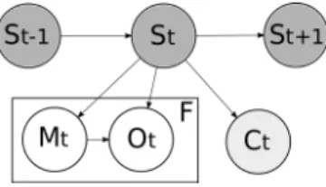
Fig. 3: Graphical Model of the framework for handling missing data. St is the hidden state, Mt represents whether
an observation has been made or not, Ot is the
correspon-ding observation, and Ct is the associated class. F is the
number of features considered. Light grey : variables that are accessible solely during the learning phase. Dark grey : variables that are never accessible.
been made. Figure 3 represents the proposed model. The following formulas hold :
p(Mtkf|Stk) ∼ Ber(mtkf)
p(Otf|Stk, Mtkf = true) ∼ ED(Otkf|Stk) p(Otf|Stk, Mtkf = f alse) ∼ δ{N oObs}
(2) Hence : p(Otf, Mtkf|Stk) = [mtkfED(Otkf|Stk)] Mtkf=true [(1 − mtkf)δ{N oObs}]Mtkf=f alse (3) Where (Mtkf = true) = 1 if Mtkf = true and 0
elsewhere.
When ED(Otkf|Stk)is a continuous distribution, the value of δ{N oObs} has to be made explicit in the implementation, but choosing the highest value available would induce nu-merical problems. To solve this, we take inspiration from a similar issue encountered with Gaussian Mixture Models, where one of the gaussian component may degenerate and evolve as a dirac. In this case, a common fix is to flatten this gaussian component, by artificially increasing its covariance matrix. By analogy, we consider that the probability of sam-pling {N oObs} is equivalent to the probability of samsam-pling an observation centred on the exact mean of a gaussian with an arbitrary covariance matrix. Provided this justification, the concrete solution is equivalent to manually fix the value of the dirac, which is now considered as a hyper-parameter of the model.
The model generalises the work exposed in [18] because when ED(Otkf|Stk)is a categorical distribution, eq 3 is also a categorical distribution. Note that the idea of using Bernoulli variables in models to work as "switches" is not new : in [13] for example, Bernoulli Mixture Models are used to discriminate the cause of an observation. Our contribution is to link it with the usage of the symbol {N oObs} for handling the MNAR issue in the continuous case.
V. APPLICATION:TRACKING A PERSON IN AN
APARTMENT
In this section, we propose to instantiate the models presented in sections III-B and IV to a practical problem : the
(a) RGB-D camera (ki-nect).
(b) A smartTile. The sen-sing floor is composed of a set of smartTiles. Fig. 4: Devices used.
2D top-view tracking of a moving person in an apartment. The observations considered are provided by several static cameras, with unknown position and orientation. The classes correspond to static areas of the apartment, and are provided by a sensing floor. No camera has the whole picture of the apartment.
A. Sensors and data
The sensors considered are RGB-D cameras (kinects, see Figure 5), which means that for each image captured, each pixel is assigned both a colour and a depth, thus each camera captures 3D scenes. Each camera has its own computational unit which extracts the position of the tracked person -approximated by the center of mass, in the relative frame of the camera. The computation of the center of mass relies on background-extraction from running-average, and blob detection.
The reference system used for classification in the lear-ning phase is a sensing floor made of SmartTiles (see Figure 4b), which are granted with four pressure detectors and a computational unit each. The informations retrieved by the SmartTiles are merged into the position of the person tracked on the ground plane, approximated by the center of pressure. Note that the center of pressure is different from the projection of the center of mass to the ground, e.g. when the person tracked is midway of a foot step. Although the center of pressure can be tracked in (R+2), we discretise the
positions in a simplification purpose.
B. Instantiation of the model
The model depicted by Figure 3 is derived for the appli-cation in the following manner. Observations correspond to the center of mass seen by the cameras (F is the number of cameras), and each class corresponds to a distinct tile composing the ground of the apartment. The classes are assessed to be MAR, while the observations are MNAR, because no camera has a field of view embracing the whole apartment. The following distributions of probabilities are chosen :
ED(Otkf|Stk) = N (µki, σki) p(Ctk|Stk) ∼ Cat(pk)
(4)
Where Cat is the categorical distribution and pkis a vector
of probabilities of presence pkjto stand over tile j while on
hidden state Sk.
The formulas used to maximise the parameters while in the M phase of the EM algorithm are the followings :
mkf = T P t=1 γ(Stk)(Mtf=true) T P t=1 γ(Stk) (5) µkf = T P t=1 γ(Stk)(Mtf=true)Otf T P t=1 γ(Stk)(Mtf=true) assuming T P t=1 γ(Stk)(Mtf = true) 6= 0 (6) σkf = T P t=1
γ(Stk)(Mtf=true)[(µkf−Otf)(µkf−Otf)T] T P t=1 γ(Stk)(Mtf=true) assuming T P t=1 γ(Stk)(Mtf = true) 6= 0 (7) pkj = T p P t=1 γ0(Stk)(Ctj=true)+ T P t=Tp+1 γ0(Stk)poldkj T P t=1 γ0(S tk) (8)
The calculation of pkj reflects the MAR aspect of the
informations retrieved by the tiles. The sum from 1 to Tp
is a sum over the data observed, the sum from Tp+ 1 to
T is a sum over the missing data. γ0(Stk) is computed
exactly the same way as γ(Stk), except that we are replacing
p(St|Ot, Mt, Ct) with p(St|Ot, Mt) when Ct is missing.
pold
kj is the last previously computed value of pkj.
C. Initialisation process
To run the EM algorithm, we first have to initialise the pa-rameters of the model (a.k.a. mtkfand the parameters related
to ED(Otkf|Stk)and p(Ctk|Stk)). This section addresses this issue.
Even though the Bayesian approach (i.e defining a prior distribution over the parameters) is elegant, it is not appli-cable to our case because of mtkf : even though its value
is comprised in range [0, 1], 0 is an adherent value, i.e. a value that is frequently met, due to the fact that the sensors have limited perception areas. Considering a continuous distribution, the probability of drawing a specific discrete event is null, so the prior over mtkfwould have to be defined
as a mixture model, e.g. :
p(mtkf) = mδ{0}+ (1 − m)B(α, β).
B(α, β) being the Beta distribution for hyper-parameters (α, β), and m a mixture coefficient that would have its own Beta prior B(α0, β0), regarding to the fact that the proportion of overlapping cameras in apartments is a-priori unknown.
The Bayesian approach would also require prior over the other parameters. We assess that the model induced would be complex enough to encounter practical issues, and that it would be nearly impossible to properly set the different
hyper-parameters. Hence we propose instead to initialise the parameters, with an instance-based technique (i.e. based on the learning dataset), by a pre-clustering.
We assume that the number of hidden states K is lower or equal to the number of classes J. We introduce the followings notations. Let J be a set of tiles {j1, j2, ...}. Let OJ be the
set of observations of dimensionality (3 × F ) seen by the set of cameras while on tiles J . Let gJ be a cluster of OJ.
At the beginning, we have a cluster g{j} of observations
O{j}per tile. We then merge together iteratively the closest
clusters with a Nearest Neighbour (NN) algorithm until there are K clusters left. Each of these K cluster then allows to compute the initial parameters of a corresponding hidden state.
To run the NN algorithm, we need to introduce a distance d. When K < J, the choice of the distance is important, since it impacts the grouping of the clusters. In turn it impacts the final solution, as EM is prone to get stuck in local-minima regarding to its initialisation. When K = J, the distance has no impact since no clusters are merged.
To define a good distance, we first note that a hidden state holds both an intrinsic information (what can see each camera per given hidden state) and an extrinsic information (what does a hidden state represent in term of position). Hence d take the form of :
d(gJ, gJ0) = rdi(gJ, gJ0) + (1 − r)de(gJ, gJ0) (9) where di and de are respectively a distance between
the intrinsic and the extrinsic informations. r is a hyper-parameter in range [0, 1], representing the relevance of intrinsic information versus extrinsic information.
The parameters that are eligible to represent the intrinsic informations of the system are mkf, µkf and σkf. We
exclude the use of µkf and σkf in the design of di as they
are not definite in the case of mkf = 0. Hence we use :
di(gJ, gJ0) = 1 F F P f =1 |mgJf− mgJ 0f| (10)
This distance tends to group together the tiles for which the cameras have similar observability. Actually, it is a pseudo-distance rather than a regular distance ([di(gJ, gJ0) = 0] ; [gJ = gJ0]), however d is still a distance if r 6= 1 and de is a distance.
The extrinsic informations of our system once the initiali-sation is done is represented by the geographic distributions of probabilities pkj, thus a good de should be able to :
— group positions that are neighbours in the 2D-plan of the apartment.
— make the system scalable to the number of clusters considered. i.e. the accuracy of the system should grow "regularly" with the number of clusters, ensuring that using a larger number of clusters (and hence, computational power) will alway be rewarded. — allow a fast convergence of the precision VS the
number of clusters used.
We design and test different de:
distance between centroids This distance simply groups the clusters that are close together.
dcentroids(gJ, gJ0) = 1
NdE(gJ, gJ0) (11)
Where N is a normalisation value so that de is
com-prised in range [0, 1], dE is the Euclideian distance,
gJ is the centroid of the tiles which are associated to
at least one observation different from {NoObs}. Ward’s distance applied to number of tiles The
War-d’s method [12] consists in minimising the augmen-tation of the variation amongst each cluster while merging them. Here we simply apply it to minimise the variation of number of tiles seen per cluster. i.e. we will tend to form clusters of similar size in term of number of tiles. dW ardT iles(gJ, gJ0) = 1 N |J ||J0| |J |+|J0|dE(gJ, gJ0) (12) Where |J | represents the number of tiles in J . Ward’s distance applied to number of observations
Assessing that the learning dataset is representative, we now apply the Ward’s method to minimise the variation of number of observations seen per cluster. i.e. we will tend to form clusters of different size, the clusters being smaller (hence giving more precise information) when the tiles it contains are frequently visited. dW ardObs(gJ, gJ0) = 1 N |OJ||OJ 0| |OJ|+|OJ 0| dE(gJ, gJ0) (13)
Where |OJ| represents the numbers of observations in
OJ.
VI. EXPERIMENTS
The learning and testing datasets consist of the centres of pressure and mass detected by the sensing ground and 4 cameras, while a person is walking in the apartment for approximately four hundred seconds. The apartment is made of 10 × 11 SmartTiles of 60 × 60 cm each, and the person walk over 68 of these tiles. Figure 5 shows the placement of the cameras in the apartment.
The criterion to stop the EM algorithm is observing the evolution of the log-likelihood being smaller than 1% between two iterations. By default, the distance used is dW ardObs, the hyper-parameter r is set to 0.5, the number
of hidden states is set to 10, the dirac value is 20, and the number of classes provided by the sensing floor is equals to the number of tiles.
Firstly, we give an insight of the behaviour of the system. Secondly, we show the efficiency of the system regarding to the number of hidden states and the distance used in the initialisation process. Thirdly, we study the scalability of the system toward the number of classes and the number of sensors. At least, we discuss the influence of some hyper-parameters.
Fig. 5: Environment and cameras used for the experiment. Cameras are represented by numbered coloured circles . Each area is numbered by the cameras which have a perception area on it. The colour of each area results from the addition of the colours of the cameras.
(a) 10 areas (b) 20 areas
Fig. 6: Figures 6a and 6b read the areas shaped by the algorithm. Each tile Cj is attributed the index k of
arg max
k
(p(Cj|Sk)) and a corresponding colour. White tiles
are not visited (presence of furnitures, ...).
A. Insight
Figures 6a and 6b reads how the different areas are shaped by the algorithm when 10 and 20 hidden states are used. Table I reads the probability of observation per hidden state and per camera when 10 hidden states are used. We make the distinction between an absolute zero probability (written as 0), and a negligible probability (written as 0.0).
Figure 6a and table I read that the areas tends to be smaller and hence to induce better precision, at places corresponding to the edge of sensors perception areas (see bottom left corner of fig 6a). This demonstrates the capability of the model to discriminate different areas, based on whether a sensor has access to information about it or not.
Figure 7 reads an example of real trajectory toward the positions assessed by the system, when 45 hidden states are used. Sensors State 0 1 2 3 4 5 6 7 8 9 Cam 1 0.7 0 0.3 0.0 0.0 0.8 0.0 0.0 0.1 0 Cam 2 0.9 0 0 0 0 0.3 0.7 0 0.2 0.3 Cam 3 0.0 0 0 0 0 0 0.9 0 0 0 Cam 4 0.0 0.4 0.2 0.1 0.9 0.3 0 0.2 0.9 0.7
TABLE I: Probabilities of making observation per hidden state, for each camera
Fig. 7: A real trajectory (red dots) toward a succession of positions assessed by the system (blue triangles). 45 hidden states are used.
B. Efficiency and influence of different distances
In this experiment, we make the number of hidden states vary and evaluate its effects on the mean error of the system, once convergence of the EM algorithm is reached.
The error is computed as the difference between the position detected by our system once learning is done (i.e. using only the cameras with the testing dataset) toward the true position of the person (which is continuous in R+2, and
is given by the sensing floor). The position detected at time t is computed as follows : pos(t) = K P k=1 [p(Stk|Ot, Mt, St−1,k0) J P j=1 pkjposT ilej] (14) Where posT ilejis the 2-D cartesian position of the centre
of the tile Cj in the 2D top-view of the apartment. We test
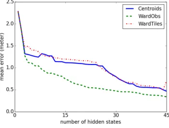
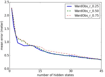
the three distances previously introduced and compare them in figure 8a. Figure 8b corresponds to the same experiment, but also shows the standard deviations.
These figures show that for 45 hidden states, we reach at best a mean error of approximately 0.34 meters using WardObs. As a reference, each state could theoretically represent an area of nbrT iles ∗ lengthT ile2/nbrStates '
0.54m2 : considering this area is a disc and that we always know with certainty what is the current state, we find a theoretical lower bound on the maximum admissible error of arg min
shape
(max(error)) ' 0.42 meters. At the limit K=J, the three distances are trivially equivalent, and the corresponding
(a) Mean error per distance vs number of hidden states
(b) Standard deviation per distance vs number of hidden states Fig. 8: Comparison between distances
mean error is approximately of 0.26 meters with a theoretical bound on the error of 0.34 meters. Thus in practice, the system doesn’t function worst than the ideal theoretical prediction.
The proposed model suffers from limitations in accuracy (as expected since it is discrete), yet we believe it is worth considering, as its generic aspect allows to easily deploy it in contexts where high precision is not required.
Figures 8a and 8b also show us that it is better to use dW ardObs rather than the other distances. It both converges
faster and doesn’t have a "plateau" for a number of hidden states comprised between 5 and 25, ensuring a more scalable behaviour. Its associated standard deviation is also better. C. Scalability
Here we test the scalability of the system to the number of discrete positions as well as the number of sensors.
Figure 9a shows the evolution of the mean error versus the precision, which is defined as the square root of the number of classes per tile of 60 × 60 cm.
(a) Precision (b) Number of sensors Fig. 9: Scalability. The graphics shows the evolution of the mean error of the system toward the precision and the number of sensors.
Counterintuitively, figure 9a shows that when the precision grows, the mean error diminishes at first, and then stop to evolve, because the distributions of presence over the tiles are not necessarily convex : as precision grows, "holes" appears inside the distributions. It is due to the limitation of our dataset, which is not extensive nor exhaustive enough to associate every discrete position to observations.
Figure 9b shows the evolution of the mean error versus the number of sensors. The mean error is computed as the average mean error for every combination of F sensors available. This figure reads that globally, the system tends to work better when the number of sensors grows. On the other side, we find that the precision of the system get always worst when we add camera 1 to any set of sensors. As camera 1 is involved in 3 out of the 6 possible combinations of two cameras, this is the reason why the mean error is higher when using two cameras instead of a single one. The inefficiency of camera 1 could be explained in the following way : its perception area is the smallest and has a lot of frontiers with others perception areas, biasing the initialisation process to cluster some of the 10 areas available in an inadequately precise fashion around it, while the rest of the apartment is clustered too roughly.
D. Influence of the hyper-parameters
We test and compared 3 different value of r as presented in figure 10. The difference of results for these different r values is not significant.
We make the dirac value vary from 1 to 191 by steps of 10, and found that it doesn’t make the mean error nor the standard deviation vary. This is probably due to the pre-clustering algorithm, which optimises the static parameters of the system (such as the probability to make observation per tile) : while in the EM algorithm, learning the sequential dependencies increases the likelihood more significantly than optimising the static parameters.
VII. CONCLUSION ANDFUTUREWORKS
In this article, we proposed to use the HMM framework to solve a multi-sensor single-person tracking problem. By doing so, we took advantage of the finite set of possible positions to correlate the proportion of missing observations with the perception areas of the sensors. We also avoided the
Fig. 10: Influence of different r values on the mean error
explicit calibration of the sensors by directly mapping the observations to the 2D-top-view map of the environment, by using an external system temporarily available that provided a map of the environment and ground truth.
The work exposed here can be extended in several ways. A first possibility would be to fuse the HMM model with a regular Kalman filter to exploit the informations gained on the perception areas of the sensors, while being able to track a person in continuous domains.
A second possibility would be to test the approach in-troduced here with others systems. For instance, we could change the classifier providing ground truth (here the sensing ground), with a mobile robot performing telemetric mapping. A third possibility would be to test if an enhancement of this model can detect false positives. A false positive, is an observation made by a sensor that should not have been made. For example, cameras detect false positives on mirrors and black surfaces reflecting a person. The problem is in principle not difficult to solve with our approach, as the classes and the observations are independent, given the hidden states, hence having more hidden states than classes may result in learning false positives. Fitting the correct number of hidden states should be sufficient to solve the problem. To do so, we would have to adapt the initialisation process to automatically detect the appropriate number of hidden states.
VIII. ACKNOWLEDGEMENTS
This paper was mainly supported by the SATELOR Project funded by the Lorraine Region and partly by the FP7 EU pro-jects CoDyCo (No. 600716 ICT 2011.2.1 Cognitive Systems and Robotics). The authors thank Serena Ivaldi, Maxime Rio and Iñaki Fernández for helpful discussions and comments on the paper.
REFERENCES
[1] Mihai Andries, Olivier Simonin, and François Charpillet. “Localisation of humans, objects and robots interacting on load-sensing floors”. In: IEEE SENSORS JOURNAL (2015).
[2] Tiziana D’Orazio and Cataldo Guaragnella. “A Survey of Automatic Event Detection in Multi-Camera Third Gener-ation Surveillance Systems”. In: InternGener-ational Journal of Pattern Recognition and Artificial Intelligence(2015). [3] Johannes Pallauf, Jörg Wagner, and Fernando Puente Leon.
“Evaluation of State-Dependent Pedestrian Tracking Based on Finite Sets”. In: IEEE Transactions on Instrumentation and Measurement(2015).
[4] Chun-Te Chu and Jenq-Neng Hwang. “Fully Unsupervised Learning of Camera Link Models for Tracking Humans Across Nonoverlapping Cameras”. In: IEEE Transactions on circuits and systems for video technology(2014). [5] Amandine Dubois. “Mesure de la fragilité et détection de
chutes pour le maintien à domicile des personnes âgées”. PhD thesis. Université de Lorraine, 2014.
[6] Lei Song and Youngcai Wang. “Multiple target counting and tracking using binary proximity sensors: bounds, coloring, and filter”. In: ACM international sumposium on Mobile and ad hoc networking and computing(2014).
[7] Rémi Emonet, Jagannadan Varadarajan, and Jean-March Odobez. “Temporal Analysis of Motif Mixtures using Dirichlet Processes”. In: IEEE Transactions on Pattern Analysis and Machine Intelligence(2013).
[8] Ahmed Kamal, Jay Farell, and Amit Roy-Chowdhury. “In-formation Weighter Consensus Filters and Their Application in Distributed Camera Networks”. In: IEEE Transactions on Automatic Control58.12 (2013).
[9] Jesse Hoey, Xiao Yang, and Marek Grzes. “Modeling and Learning for LaCasa, the Location And Context-Aware Safety Assistant”. In: NIPS Workshop on Machine Learning Approaches to Mobile Context Awareness(2012).
[10] Rudy Raymond, Tetsuro Morimura, and Takayaki Osogami. “Map Matching with Hidden Markov Model on Sampled Road Networks”. In: 21st International Conference on Pat-tern Recognition (ICPR)(2012), pp. 2242–2245.
[11] Balhador Khaleghi et al. “Multisensor data fusion: A review of the state-of-the-art”. In: Information Fusion 14 (2011), p. 562.
[12] Fionn Murtagh and Pierre Legendre. “Ward’s Hierarchical Clustering Method: Clustering Criterion and Agglomerative Algorithm”. In: eprint arXiv:1111.6285v2 (2011).
[13] Adria Gimenez and Alfons Juan. “Embedded Bernoulli Mixture HMMs for Handwritten Word Recognition”. In: International Conference on Document Analysis and Recog-nition, 2009 (ICDAR)(2009), pp. 896–900.
[14] Paul Newson and John Krumm. “Hidden Markov Map Matching Through Noise and Sparseness”. In: International Conference on Advances in Geographic Information Systems (ACM SIGSPATIAL)(2009), pp. 336–343.
[15] Yunyoug Nam et al. “Learning Spatio-Temporal Topology of a Multi-Camera Network by Tracking Multiple People”. In: International Journal of Computer, Electrical, Automation, Control and Information Engineering(2007).
[16] Christopher M. Bishop. Pattern Recognition and Machine Learning. Ed. by Springer. Information Science and Statis-tics, 2006.
[17] Lin Liao, Dieter Fox, and Henry Kautz. “Location-Based Activity Recognition using Relational Markov Networks”. In: Proceedings of the 19th international joint conference on Artificial intelligence (IJCAI)(2005).
[18] Shun-Zheng Yu and Hisashi Kobayashi. “A hidden semi Markov model with missing data and multiple observation sequences for mobility tracking”. In: Signal Processing 83.2 (2003), pp. 235 –250.
[19] A. P. Dempster, N. M. Laird, and Donald Rubin. “Maximum Likelihood from Incomplete Data via the EM Algorithm”. In: Journal of the Royal Statistical Society 39.1 (1977), pp. 1–38.