Publisher’s version / Version de l'éditeur:
Vous avez des questions? Nous pouvons vous aider. Pour communiquer directement avec un auteur, consultez la
première page de la revue dans laquelle son article a été publié afin de trouver ses coordonnées. Si vous n’arrivez pas à les repérer, communiquez avec nous à PublicationsArchive-ArchivesPublications@nrc-cnrc.gc.ca.
Questions? Contact the NRC Publications Archive team at
PublicationsArchive-ArchivesPublications@nrc-cnrc.gc.ca. If you wish to email the authors directly, please see the first page of the publication for their contact information.
https://publications-cnrc.canada.ca/fra/droits
L’accès à ce site Web et l’utilisation de son contenu sont assujettis aux conditions présentées dans le site LISEZ CES CONDITIONS ATTENTIVEMENT AVANT D’UTILISER CE SITE WEB.
The Genetic and Evolutionary Computation Conference (GECCO-2007), 2007
READ THESE TERMS AND CONDITIONS CAREFULLY BEFORE USING THIS WEBSITE.
https://nrc-publications.canada.ca/eng/copyright
NRC Publications Archive Record / Notice des Archives des publications du CNRC :
https://nrc-publications.canada.ca/eng/view/object/?id=b8012765-9292-40b2-921d-7a499df44ced
https://publications-cnrc.canada.ca/fra/voir/objet/?id=b8012765-9292-40b2-921d-7a499df44ced
NRC Publications Archive
Archives des publications du CNRC
This publication could be one of several versions: author’s original, accepted manuscript or the publisher’s version. / La version de cette publication peut être l’une des suivantes : la version prépublication de l’auteur, la version acceptée du manuscrit ou la version de l’éditeur.
Access and use of this website and the material on it are subject to the Terms and Conditions set forth at
Computational intelligence techniques: a study of scleroderma skin
disease
Computational Intelligence Techniques: A
Study of Scleroderma Skin Disease *
Valdés, J., and Barton, A.
July 7-11, 2007
* proceedings of GECCO Late-Breaking Paper. GECCO 2007
Conference. London, England. July 7-11, 2007. NRC 49293.
Copyright 2007 by
National Research Council of Canada
Permission is granted to quote short excerpts and to reproduce figures and tables from this report, provided that the source of such material is fully acknowledged.
Computational Intelligence Techniques: A Study of
Scleroderma Skin Disease
Julio J. Valdes
julio.valdes@nrc-cnrc.gc.ca
alan.barton@nrc-cnrc.gc.ca
Alan J. Barton
National Research Council Canada Institute for Information Technology
M50, 1200 Montreal Rd. Ottawa, ON K1A 0R6
ABSTRACT
This paper presents an analysis of microarray gene expres-sion data from patients with and without scleroderma skin disease using computational intelligence and visual data min-ing techniques. Virtual reality spaces are used for providmin-ing unsupervised insight about the information content of the original set of genes describing the objects. These spaces are constructed by hybrid optimization algorithms based on a combination of Differential Evolution (DE) and Par-ticle Swarm Optimization respectively, with deterministic Fletcher-Reeves optimization. A distributed-pipelined data mining algorithm composed of clustering and cross-validated rough sets analysis is applied in order to find subsets of rele-vant attributes with high classification capabilities. Finally, genetic programming (GP) is applied in order to find ex-plicit analytic expressions for the characteristic functions of the scleroderma and the normal classes. The virtual reality spaces associated with the set of function arguments (genes) are also computed. Several small subsets of genes are discov-ered which are capable of classifying the data with complete accuracy. They represent genes potentially relevant to the understanding of the scleroderma disease.
Categories and Subject Descriptors
I.5 [Computing Methodologies]: Pattern Recognition; E.0 [Data]: General; J.3 [Computer Applications]: Life and Medical Sciences
General Terms
Experimentation
Keywords
visual data mining, virtual reality spaces, differential evo-lution, particle swarm optimization, hybrid evolutionary-classical optimization, similarity structure preservation, clus-tering, rough sets, genetic programming, grid computing, genomics, Scleroderma disease
Copyright 2007 Crown in Right of Canada.
This article was authored by employees of the National Research Council of Canada. As such, the Canadian Government retains all interest in the copyright to this work and grants to ACM a nonexclusive, royalty-free right to publish or reproduce this article, or to allow others to do so, provided that clear attribution is given both to the NRC and the authors.
GECCO’07,July 7–11, 2007, London, England, United Kingdom. ACM 978-1-59593-697-4/07/0007.
1.
INTRODUCTION
Scleroderma is a complex and sometimes fatal disease. Its pathogenesis is poorly understood and the development of the disease is known to involve the immune system, the vasculature, and extracellular matrix deposition. Unfortu-nately, there are no definitive markers or curative treatments [23]. Scleroderma can occur in a localized form confined to the skin or a systemic form referred to as systemic sclerosis (SSc), which involves internal organs and the skin. When the disease affects critical internal organs it may lead to death. In more than 90% of the patients the skin is affected and cutaneous involvement closely correlates with internal organ pathology. The disease is most prevalent in women with a median age. Symptoms develop symmetrically and include swelling in the hands and Raynauds phenomenon. The skin becomes tense, shiny, and painful. Skin changes progress and may involve the face, trunk, and lower extrem-ities. The edematous skin becomes fibrotic and hardens. These distressing skin changes are generally accompanied by internal organ involvement. Studies of gene expression in the skin of individuals affected with diffuse scleroderma and their comparison with a similar characterization made on biopsies from normal, unaffected individuals have been conducted. The goal is to find markers for the disease and in this paper a knowledge discovery approach using evolu-tionary computation and other techniques is presented.
First, visual data mining with virtual reality (VR) spaces are used for representing the original set of genes describing the objects (in an unsupervised manner). Their construction uses hybrid optimization algorithms combining Differential Evolution (DE) and Particle Swarm Optimization (PSO) with classical deterministic Fletcher-Reeves optimization. Then, a distributed-pipelined data mining algorithm (DP-DM) is applied in order to find subsets of relevant attributes with high classification capabilities. VR spaces are com-puted for selected subsets of genes and their structure is analyzed in comparison with the scleroderma and normal class distributions. Finally, genetic programming (GP) is applied in order to find explicit analytic expressions for com-puting the characteristic functions of the scleroderma and the normal classes. The VR spaces associated with the set of function arguments (genes) are also computed.
2.
VISUAL DATA MINING
The role of visualization techniques in the knowledge dis-covery process is well known. Several reasons make VR a
suitable paradigm: It is flexible, allows immersion, creates a living experience and is broad and deep (the user may see the VR world as a whole, and/or concentrate the attention on specific details). Of no less importance is the fact that in or-der to interact with a virtual world, no specialized technical expertise is required. A virtual reality technique for visual data mining on heterogeneous, imprecise and incomplete in-formation systems extending the concept of 3D modelling to relational structures was introduced in [21], [22].
A virtual reality space can be defined as a tuple Υ =< O, G, B,ℜm, g
o, ϕ, gr, b, r >, where O is a relational structure (O =< O, Γv>, O is a finite set of objects, and Γv is a set of relations); G is a non-empty set of geometries representing the different objects and relations; B is a non-empty set of behaviors of the objects in the virtual world; ℜm
⊂ Rm is a metric space of dimension m (euclidean or not) which will be the actual virtual reality geometric space. The other elements are mappings: go: O → G, ϕ : O → ℜm, gr: Γv→ G, b : O → B.
If the objects are in a heterogeneous space, ϕ : ˆHn → ℜm. Several desiderata can be considered for building a VR-space. One may be to preserve one or more properties from the original space as much as possible (for example, the similarity structure of the data [4]). From an unsu-pervised perspective, the role of ϕ could be to maximize some metric/non-metric structure preservation criteria [2], or minimize some measure of information loss. From a su-pervised point of view ϕ could be chosen as to emphasize some measure of class separability over the objects in O [22]. In particular, if δij is a dissimilarity measure between any two i, j ∈ U (i, j ∈ [1, N], where n is the number of ob-jects), and ζivjv is another dissimilarity measure defined on
objects iv, jv
∈ O from Υ (iv = ξ(i), jv = ξ(j), they are in one-to-one correspondence), an error measure frequently used is Sammon error [18]:
Sammon error = P 1 i<jδij P i<j(δij− ζij)2 δij (1)
3.
EVOLUTIONARY ALGORITHMS
3.1
Differential Evolution
Differential Evolution [19], [17], [9] is a kind of evolution-ary algorithm working with real-valued vectors, and it is rel-atively less popular than genetic algorithms (GA). Like GA, evolution strategies and other EC algorithms, it works with populations of individual vectors (real-valued), and evolves them. Many variants have been introduced (called strate-gies), but the general scheme is as follows:
Algorithm 1. General Differential Evolution Scheme (0) Initialization: Create a population P of random
vec-tors in ℜn
, and choose an objective function f : ℜn → ℜ and a strategy S, involving vector differentials. (1) Choose a target vector from the population ~xt∈ P. (2) Randomly choose a set of other population vectors V =
{~x1, ~x2, . . .} with a cardinality determined by S. (3) Apply strategy S to the set of vectors V ∪{~xt} yielding
a new vector ~xt′.
(4) Add ~xt or ~xt′ to the new population according to the
value of the objective function f and the type of prob-lem (minimization or maximization).
(5) Repeat steps 1-4 to form a new population until ter-mination conditions are satisfied.
— End of Algorithm —
3.2
Particle Swarm Optimization
Particle swarm optimization (PSO) is a population-based stochastic search process, modeled after the social behavior of bird flocks and similar animal collectives [10][11]. The al-gorithm maintains a population of particles, where each par-ticle represents a potential solution to an optimization prob-lem. In the context of PSO, a swarm refers to a number of potential solutions to the optimization problem, where each potential solution is referred to as a particle. Each particle i maintains information concerning its current position and velocity, as well as its best location overall. These elements are modified as the process evolves, and different strategies have been proposed for updating them, which consider a va-riety of elements like the intrinsic information (history) of the particle, cognitive and social factors, the effect of the neighborhood, etc, formalized in different ways. The swarm model used has the form proposed in [13]
νidk+1= ω · ν k id+ φ1· (p k id− x k id) + φ2· (p k gd− x k id) xk+1 id = x k id+ νidk+1 φi= bi· ri+ di, i = 1, 2 (2) where νk+1
id is the velocity component along dimension d for particle i at iteration k + 1, and xk+1
id is its location; b1 and b2 are positive constants equal to 1.5; r1 and r2 are random numbers uniformly distributed in the range (0, 1); d1 and d2 are positive constants equal to 0.5, to cooperate with b1 and b2 in order to confine φ1 and φ1 within the interval (0.5, 2); ω is an inertia weight.
3.3
Genetic Programming
Analytic functions are among the most important build-ing blocks for modelbuild-ing, and are a classical form of knowl-edge. Direct discovery of general analytic functions can be approached from a computational intelligence perspective via evolutionary computation. Genetic programming tech-niques aim at evolving computer programs, which ultimately are functions. Genetic Programming is an extension of the Genetic Algorithm introduced in [12].
Those programs which represent functions are of partic-ular interest and can be modeled as y = F (x1, · · · , xn), where (x1, · · · , xn) is the set of independent or predictor variables, and y the dependent or predicted variable, so that x1, · · · , xn, y ∈ R, where R are the reals. The function F is built by assembling functional subtrees using a set of prede-fined primitive functions (the function set), deprede-fined before-hand. In general terms, the model describing the program is given by y = F (~x), where y ∈ R and ~x ∈ Rn. Classical implementations of genetic programming for modeling use a tree representation for the expressions along with their associated tree operations (GPStudio (GPS) [3]). Others, like gene expression programming (GEP) [6] encode expres-sions as strings of fixed length. For the interplay of the chromosomes and the expression trees (ET), GEP uses a translation system to transfer the chromosomes into expres-sion trees and vice versa [6]. The set of genetic operators applied to chromosomes always produces valid ETs.
The chromosomes in GEP itself are composed of genes structurally organized in a head and a tail [5]. The head
contains symbols that represent both functions (from a func-tion set F) and terminals (from a terminal set T), whereas the tail contains only terminals. Two different alphabets occur at different regions within a gene. For each problem, the length of the head h is chosen, whereas the length of the tail t is a function of h and the number of arguments of the function with the largest arity. Both the classical and GEP approaches to genetic programming are investigated.
4.
CLASSICAL OPTIMIZATION
The Fletcher-Reeves method is a well known technique used in deterministic optimization [16]. It assumes that the function f is roughly approximated as a quadratic form in the neighborhood of a N dimensional point P. f (~x) ≈ c − ~b · ~x +1
2~x · A · ~x, where c ≡ f(P), b ≡ −∇f|P and [A]ij ≡ ∂
2f
∂xi∂xj|P The matrix A whose components are the second partial derivatives of the function is called the Hes-sian matrix of the function at P. Starting with an arbitrary initial vector ~g0and letting ~h0= ~g0, the conjugate gradient method constructs two sequences of vectors from the recur-rence ~gi+1= ~gi− λiA· ~hi, ~hi+1= ~gi+1− γiA· ~hi, where i = 0, 1, 2, . . . The vectors satisfy the orthogonality and con-jugacy conditions ~gi· ~gj= 0, ~hi· A · ~hj= 0, ~gi· ~hj= 0, j < i and λi, γi are given by λi=
~gi·~gj ~hi·A·~hi, γi= ~ gi+1·~gi+1 ~ gi·~gi .
It can be proven [16] that if ~hiis the direction from point Pi to the minimum of f located at Pi+1, then ~gi+1 = −∇f(Pi+1), therefore, not requiring the Hessian matrix.
5.
HYBRID OPTIMIZATION
Evolutionary algorithms are global optimizers and in gen-eral explore broad areas of the search space, whereas clas-sical deterministic optimization techniques are more pow-erful at local search, exploiting the knowledge of the par-tial derivatives of the function. It is a common practice to combine them in hybrid algorithms which benefit from the good properties of both approaches. A first hybrid algorithm (DE-FR) was constructed by applying DE until convergence and then using the final solution as initial approximation for the Fletcher-Reeves algorithm. A second hybrid algorithm (PSO-FR) was constructed in the same way, but using PSO, instead of DE. These hybrid algorithms were used for the implicit computation of the l mapping required by the VR spaces (minimization of the Sammon error in Eq-1).
6.
DISTRIBUTED PIPELINE DATA MINING
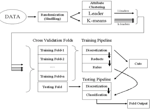
A data mining methodology based on a distributed pipeline of algorithms for finding relevant subsets of at-tributes in highly-dimensional information systems was in-troduced in [20]. The general idea is to construct subsets of relatively similar attributes, such that a simplified repre-sentation of the data objects is obtained by using the cor-responding attribute subset representatives. The attributes of these simplified information systems are explored from a rough set perspective [15], [14] by computing their reducts (subsets of the original attributes with the same classi-fication capability as the whole set). From them, rules are learned and applied systematically to testing data sub-sets not involved in the learning process following a cross-validation scheme (Fig-1), in order to better characterize the
classification ability of the retained attributes. The whole procedure can be seen as a pipeline.
In a first step, the objects in the dataset are shuffled using a randomized approach in order to reduce the possible bi-ases introduced within the learning process by data chunks sharing the same decision attribute. Then, the attributes of the shuffled dataset are clustered using two families of clus-tering procedures: i) three variants of the leader algorithm [8] (forward, reverse and absolute best), and four variants of k-means [1] (Forgy, Jancey, convergent and MacQueen). The leader and the k-means algorithms were used with a similarity measure rather than with a distance; in particu-lar Gower’s general coefficient was used [7].
Each of the formed clusters of attributes is represented by exactly one of the original data attributes. By the nature of the leader algorithm, the representative is the leader (called an l-leader ), whereas for a k-means algorithm, a cluster is represented by the most similar object w.r.t. the centroid of the corresponding cluster (the k-leader ). As a next step, a new information system is built from the original by retain-ing the l-leaders (or the k-leaders). The filtered informa-tion system undergoes a segmentainforma-tion with the purpose of learning classification rules, and testing their generalization ability in a cross-validation framework. N-folds are used as training sets; where the numeric attributes present are con-verted into nominal attributes via a discretization process, and from them, reducts are constructed. Finally, classifi-cation rules are built from the reducts, and applied to a discretized version of the test fold (according to the cuts ob-tained previously), from which the generalization ability of the generated rules is evaluated. Each stage feeds its results to the next stage of processing, yielding a pipelined data analysis stream. This methodology had been used success-fully in the analysis of gene expression data [20].
Distributed and Grid computing is an obvious choice for many data mining tasks within the knowledge discovery pro-cess. For this study, Condor (http://www.cs.wisc.edu/ condor/), which is a specialized workload management sys-tem for compute-intensive jobs in a distributed comput-ing environment, developed at the University of Wisconsin-Madison (UW-Wisconsin-Madison) was used.
7.
EXPERIMENTAL SETTINGS
The data used in the study was the human scleroderma microarray dataset consisting of 27 samples coming from normal patients and patients affected by scleroderma. A set of 7777 genes characterizes each sample. See [23] for details. In order to make a preliminary assessment about the rela-tion between the data structure as condirela-tioned by the 7777 genes and the class distribution, unsupervised virtual reality spaces for visual data mining were computed. Two kinds of experiments were made: i) the DE and PSO methods were applied separately and ii) the two hybrid algorithms (DE-FR and PSO-(DE-FR) were applied.
In the case of DE, vectors of dimension equal to 27x3 = 81 were used in order to make their elements be the coor-dinates of the objects in the VR space. The popula-tion size was fixed as 500 such vectors, and the num-ber of generations was set to 500 as well. The fol-lowing DE strategies were applied: {DE/rand/1/exp, DE/rand-to-best/1/exp, DE/best/2/exp, DE/rand/2/exp, DE/best/1/bin, DE/rand/1/bin, DE/rand-to-best/1/bin, DE/best/2/bin DE/rand/2/bin}. The set of scaling factors
Figure 1: Data processing strategy combining clustering, Rough Sets analysis and crossvalidation.
F spanned the range [0.1, 1] with 0.1 intervals, the crossover ratio covered the same set of values and five seeds were used for creating the sets of random numbers used by the proce-dure {−101, 8943, 98438, 84376, 539}.
For PSO, the dimension of the particles was set equal to that of the DE vectors. The number of particles and the number of generations were equal to the DE population size and the number of generations respectively. The ini-tial and final weights values were {0.1, 0.2, 0.4, 0.6, 0.8, 0.9} respectively and the particle maximum velocity values were {0.1, 0.15, 0.20, 0.25, 0.30}. The set of seeds was the same as the one used in DE in order to ensure comparability of the results. The objective function was Eq-1 using Gower’s similarity [7] in the space of the original attributes (genes) and Euclidean distance in the VR space.
The pipeline (Fig. 1) was investigated through the gener-ation of 2880 k-leader and 1320 l-leader for a total of 4200 experiments (Table 1). The discretization, reduct compu-tation and rule generation algorithms are those included in the Rosetta system [14].
GPS was used with the following settings: function set {+, −, ∗, /, exp}, random constants in the range [0, 100], pop-ulation size = 100, 000, reproduction probability = 0.05, mu-tation probability = 0.1, crossover probability = 0.85 and tree depth = 6. The fitness function was defined as the mean absolute error. GEP was applied in all cases by allowing the generation of random constants in the range [−10, 10] with population size = 30, the use of a non-terminal function set {+, −, ∗, /, exp, √ , ln}, and 4 genes linked with addition. The fitness function was defined as the classification error.
8.
RESULTS
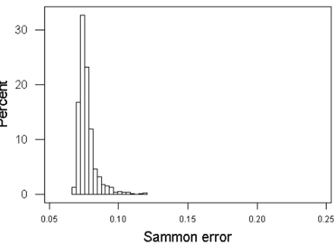
The distributions of Sammon errors for the VR spaces computed with DE and PSO exclusively are shown in Fig. 2(a) and Fig. 2(b). They are both highly skewed towards the lower error end, but the DE covers a broader error range
w.r.t the PSO and also is multimodal. This is related with the variability introduced by the large set of different DE strategies used, some of which have large interquartile ranges.
Clearly, it is impossible to represent virtual reality spaces on a static medium. A comparative composition of snap-shots of the VR spaces using the best solutions found by the DE and PSO (independently) and combined with Fletcher-Reeves is shown in Figs. 2(c), 2(d), 2(e), 2(f). Dark spheres were used to indicate the location of scleroderma samples and light ones represent those of the normal class. Also, convex hulls are included as aids for visualizing the class dis-tribution, but this information is only of comparative value, as the class information was not used in the computation of the VR space. Fig. 2(c) shows that 3 nonlinear new features computed out of the 7777 original genes by DE alone are capable of reasonably distinguish the two classes, although with an important overlap. When this solution is refined by the deterministic, Fletcher-Reeves algorithm, the final solution shown in Fig. 2(d) presents a very clear class dif-ferentiability, as the classes are almost linearly separable (in that particular nonlinear space). In the case of PSO, the im-provement of its hybridization with the FR technique is even larger than for the DE case (Figs. 2(e), 2(f)). The solution of the hybrid algorithm presents a space in which the two classes appear naturally separated (that is, using only the in-formation contained in the original genes for computing the 3 nonlinear features and not the class attribute). The DE-FR and PSO-DE-FR results show that there are genes within the 7777 original carrying discrimination information.
When the DP-DM technique was used for finding sub-sets of relevant genes, the results shown in Table-2 and Table-3 were obtained. Some of the subsets have high ac-curacies when predicting the scleroderma and the normal classes and among them three were selected for a detailed analysis. Experiments 986, 2609 and 2054 (accuracy range = [0.846, 0.857]) contain 58, 30 and 80 genes respectively. In
(a) Sammon error distribution for unsupervised solutions
obtained with Differential Evolution (DE). (b) Sammon error distribution for unsupervised solutionsobtained with Particle Swarm Optimization (PSO).
(c) Best space obtained by DE only. (Sammon error:
0.0666) (d) Best space obtained by a hybrid algorithm (DE +Fletcher-Reeves). (Sammon error: 0.0665)
(e) Best space obtained by PSO
only. (Sammon error: 0.0680) (f) Best space obtained by a Hybrid algorithm (PSO + Fletcher-Reeves). (Sammon error: 0.06625) Figure 2: Distribution of Sammon errors and selected best virtual reality spaces representing the original 27 x 7777 data. Dark objects = samples from the scleroderma class. Light objects = normal samples.
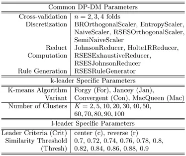
Table 1: The set of parameters and values used in the4200 experiments with the 27 by 7777 sclero-derma skin data set using DP-DM. The Discretiza-tion, Reduct Computation and Rule Generation al-gorithms are from within the Rosetta system.
Common DP-DM Parameters Cross-validation n = 2, 3, 4 folds
Discretization BROrthogonalScaler, EntropyScaler, NaiveScaler, RSESOrthogonalScaler, SemiNaiveScaler
Reduct JohnsonReducer, Holte1RReducer, Computation RSESExhaustiveReducer,
RSESJohnsonReducer Rule Generation RSESRuleGenerator
k-leader Specific Parameters K-means Algorithm Forgy (For), Jancey (Jan),
Variant Convergent (Con), MacQueen (Mac) Number of Clusters K = 2, 5, 10, 20, 30, 40, 50,
60, 70, 80, 90, 100 l-leader Specific Parameters Leader Criteria (Crit) center (c), reverse (r)
Similarity Threshold 0.7, 0.72, 0.74, 0.76, 0.78, 0.8, (Thresh) 0.82, 0.84, 0.86, 0.88, 0.9
order to visualize the relation between their information con-tent as revealed by their similarity structure and the class distribution, VR spaces were computed Figs. 3(a), 3(c) and 3(e). They show clearly the differentiation of the sclero-derma and the normal classes, but now based on a much smaller set of genes. These subsets of genes were used in genetic programming experiments with the GEP technique for finding analytic expressions for the characteristic func-tion of the classes using these subsets of genes as predictor variables. In these experiments, 80% of the samples were used for learning and the remaining 20% as independent test. The resulting expressions are given by Eqs-4, 6, 5, to-gether with the decision rule for classification. In all cases the corresponding expressions discovered by GP performed with 100% accuracy on both the learning and the test sets. This result, although very positive, should be taken with caution due to the limited number of samples available and the fact that there is a high number of replicate samples taken from an even smaller number of patients [23]. It is interesting to observe that an even smaller number of genes from each subset is necessary for constructing perfectly clas-sifying functions in all cases. In a final experiment, the VR spaces corresponding exclusively to those genes involved in the characteristic functions were computed (Figs. 3(b), 3(d) and 3(f)). The natural separation between the classes is very clear in all cases, explaining why the found character-istic functions present a very simple algebraic structure, in spite of the broad set of terminal functions and constants allowed during the search process.
The characteristic function found using gene expression programming is of the following general form. Object class membership will be determined by the function f (· · · ) as-suming a value above or below the specified threshold.
Table 2: Selected pipeline l-leader n-fold cross-validated experiments with maximum accuracy > 0.85 using the 27 by 7777 dataset. Sorted by decreas-ing minimum accuracy. See Table-1 for abbreviation definitions. See Table-3 for the k-leader results.
best l-leader experiments (max > 0.85)
Exp mean median std dev min max n-Folds Crit Thresh
986 0.82 0.78 0.14 0.71 1 4 r 0.86 985 0.82 0.78 0.14 0.71 1 4 c 0.86 981 0.82 0.84 0.07 0.71 0.86 4 c 0.82 982 0.82 0.84 0.07 0.71 0.86 4 r 0.82 964 0.81 0.78 0.17 0.67 1 3 r 0.86 963 0.81 0.78 0.17 0.67 1 3 c 0.86 583 0.81 0.78 0.15 0.67 1 4 c 0.8 584 0.81 0.78 0.15 0.67 1 4 r 0.8 365 0.78 0.78 0.11 0.67 0.89 3 c 0.82 366 0.78 0.78 0.11 0.67 0.89 3 r 0.82 1026 0.78 0.78 0.11 0.67 0.89 3 r 0.82 1025 0.78 0.78 0.11 0.67 0.89 3 c 0.82 36 0.78 0.78 0.11 0.67 0.89 3 r 0.82 629 0.78 0.78 0.11 0.67 0.89 3 c 0.82 630 0.78 0.78 0.11 0.67 0.89 3 r 0.82 35 0.78 0.78 0.11 0.67 0.89 3 c 0.82 515 0.74 0.71 0.08 0.67 0.86 4 c 0.78 516 0.74 0.71 0.08 0.67 0.86 4 r 0.78
Table 3: Selected pipeline k-leader n-fold cross-validated experiments with maximum accuracy > 0.85 using the 27 by 7777 dataset. Sorted by decreas-ing minimum accuracy. See Table-1 for abbreviation definitions. See Table-2 for the l-leader results.
best k-leader experiments (max > 0.85) Exp mean median std dev min max n-Folds Alg K 2609 0.92 0.92 0.004 0.92 0.93 2 For 30 2610 0.92 0.92 0.004 0.92 0.93 2 Jan 30 2657 0.92 0.89 0.064 0.89 1 3 For 30 2658 0.92 0.89 0.064 0.89 1 3 Jan 30 2081 0.92 0.89 0.064 0.89 1 3 For 30 2082 0.92 0.89 0.064 0.89 1 3 Jan 30 2130 0.93 0.93 0.082 0.86 1 4 Jan 30 2129 0.93 0.93 0.082 0.86 1 4 For 30 2705 0.93 0.93 0.082 0.86 1 4 For 30 2706 0.93 0.93 0.082 0.86 1 4 Jan 30 predictedClass = ½ scleroderma iff (· · · ) ≥ 0.5 normal otherwise
Three datasets were selected from the results of the DP-DM processing by selecting the best l-leader and k-leader re-sults and the first k-leader result that had a value of K differ-ent from the best; namely experimdiffer-ents 2609, 986, and 2054 respectively (See Table-3 for the best k-leader results and Table-2 for the best l-leader results). Each of the datasets was partitioned into a training set (22) and a test set (5).
The best k-leader experiment, 2609, containing 30 at-tributes was used for learning using two genetic
program-ming algorithms. An experiment using GPStudio [3] yielded 100% accuracy on the training and test sets. Eq. 3 shows the characteristic function for the two scleroderma classes.
f (v4802, v3015, v1026, v6215, v7396, v1787, v417, v220) = exp(¡(v1787− v417) ∗ (k1/exp(v1026/(v220+ v7396)))¢∗ ¡(v1787∗v417)+(v3015/v4802)¢/exp(exp(exp(exp(k2−v6215)))))
(3)
where k1= 0.803200238292664 and k2= 0.711840419895873. While with GEP the characteristic function in Eq. 4 was also able to achieve 100% accuracy on the training and test sets, sharing a variable (v6215) with the GPStudio result. f (v164, v459, v1692, v6215) = 2 · v6215+ v459∗ v1692+ exp (v164)
(4)
The best l-leader experiment, 986, containing 58 attributes was used with the same ratio of training to test set objects (80/20), which lead (by GEP) to the following characteristic function that was able to achieve 100% accuracy on both the training and test sets.
f (v666, v2026, v5333, v6443, v6665, v7125, v7300, v7334) = 2 · v7300+ v6665+ v666− v5333+ v6443− v7334+ v7125+ v2026
(5)
One further k-leader experiment, 2054, was selected that contained 80 attributes. The derived characteristic function was also able to achieve 100% on both training and test sets.
f (v4, v400, v459, v1209, v1787, v2026, v2227, v4563, v5046, v5868, v7177) = 2·vv400 4 +v1787−(v1209− v4563)+v2026+v7177+v5868+v5046v459 (6)
9.
CONCLUSION
An evolutionary computation based methodology using clustering, rough sets analysis, genetic programming and gene expression programming, differential evolution and par-ticle swarm optimization with distributed computing has been applied to scleroderma data leading to the identifica-tion of subsets of genes that lead to separaidentifica-tion of diseased and normal samples. Further investigation of the biologi-cal significance of such genes would need to be performed. Other classifications of the data are also possible and they could potentially lead to further insight into this disease.
10.
REFERENCES
[1] M. Anderberg. Cluster Analysis for Applications, page 359. Academic Press, 1973.
[2] I. Borg and J. Lingoes. Multidimensional similarity structure analysis. Springer-Verlag, 1987.
[3] BridgerTech, Inc., http://www.bridgertech.com. GP Studio 2.4: User Guide, 2007.
[4] J. L. Chandon and S. Pinson. Analyse typologique. Th´eorie et applications. Masson, Paris, 1981. [5] C. Ferreira. Gene expression programming: A new
adaptive algorithm for problem solving. Journal of Complex Systems, 13(2):87–129, 2001.
[6] C. Ferreira. Gene Expression Programming: Mathematical Modeling by an Artificial Intelligence. Angra do Heroismo, Portugal, 2002.
[7] J. C. Gower. A general coefficient of similarity and some of its properties. Biometrics, 1(27):857–871, 1973.
[8] J. Hartigan. Clustering Algorithms, page 351. John Wiley & Sons, 1975.
[9] R. S. K. Price and J. Lampinen. Differential Evolution : A Practical Approach to Global Optimization. Natural Computing Series. Springer Verlag, 2005. [10] J. Kennedy and R. C. Eberhart. Particle swarm
optimization. In Proceedings of the IEEE International Joint Conference on Neural Networks, volume 4, pages 1942–1948, 1995.
[11] J. Kennedy, R. C. Eberhart, and Y. Shi. Morgan Kaufmann, 2002.
[12] J. Koza. Hierarchical genetic algorithms operating on populations of computer programs. In Proceedings of the 11-th International Joint Conference on Artificial Intelligence, volume 1, pages 768–774, 1989.
[13] Y. ling Zheng, L. hua Ma, L. yan Zhang, and J. xin Qian. Study of particle swarm optimizer with an increasing inertia weight. In Proceedings of the World Congress on Evolutionary Computation, pages 221–226, Canberra, Australia, Dec 8-12, 2003, 2003. [14] A. Øhrn and J. Komorowskii. Rosetta- a rough set
toolkit for the analysis of data. In Proc. of Third Int. Join Conf. on Information Sciences (JCIS97), pages 403–407, Durham, NC, USA, March 1-5, 1997, 1997. [15] Z. Pawlak. Rough sets: Theoretical aspects of
reasoning about data. Kluwer Academic Pub., 1991. [16] W. Pres, B. Flannery, S. Teukolsky, and
W. Vetterling. Numeric Recipes in C. Cambridge University Press, 1992.
[17] K. Price. Differential evolution: a fast and simple numerical optimizer. In J. K. J. Y. M. Smith, M. Lee, editor, 1996 Biennial Conference of the North American Fuzzy Information Processing Society, NAFIPS, pages 524–527. IEEE Press, June 1996. [18] J. W. Sammon. A non-linear mapping for data
structure analysis. IEEE Trans. Computers, C18:401–408, 1969.
[19] R. Storn and K. Price. Differential evolution - a simple and efficient adaptive scheme for global optimization over continuous spaces. Technical Report TR-95-012, ICSI, March 1995.
[20] J. J. Valde´es and A. J. Barton. Relevant attribute discovery in high dimensional data based on rough sets and unsupervised classification: Application to leukemia gene expressions. Lecture Notes in Artificial Intelligence. Springer-Verlag, (3641):362–371, 2005. [21] J. J. Vald´es. Virtual reality representation of
relational systems and decision rules:. In P. Hajek, editor, Theory and Application of Relational Structures as Knowledge Instruments, Prague, Nov 2002. Meeting of the COST Action 274.
[22] J. J. Vald´es. Virtual reality representation of information systems and decision rules:. In Lecture Notes in Artificial Intelligence, volume 2639 of LNAI, pages 615–618. Springer-Verlag, 2003.
[23] M. L. Whitfield, D. R. Finlay, J. I. Murray, O. G. Troyanskaya, J.-T. Chi, A. Pergamenschikov, T. H. McCalmont, P. O. Brown, D. Botstein, and M. K. Connolly. Systemic and cell type-specific gene expression patterns in scleroderma skin. PNAS, 100(21):12319–12324, 2003.
(a) k-leader Experiment 2054 with
80 genes. (Sammon error: 0.04485) (b) k-leader Experiment 2054 with 11genes appearing in Eq-6. (Sammon error: 0.0231)
(c) k-leader Experiment 2609 with 30 genes. (Sammon error: 0.03407)
(d) k-leader Experiment 2609 with 4 genes appearing in Eq-4. (Sammon er-ror: 0.03102)
(e) l-leader Experiment 986 with 58 genes. (Sammon er-ror: 0.04424)
(f) l-leader Experiment 986 with 8 genes appearing in Eq-5. (Sam-mon error: 0.06038)
Figure 3: Selected best virtual reality spaces representing the original 27 x 7777 data. Dark objects = samples from the scleroderma class. Light objects = normal samples.