Variation of phytoplankton absorption coefficients in the northern South China Sea during spring and autumn

HAL Id: hal-00297894

https://hal.archives-ouvertes.fr/hal-00297894

HAL is a multi-disciplinary open access

archive for the deposit and dissemination of sci-entific research documents, whether they are pub-lished or not. The documents may come from teaching and research institutions in France or abroad, or from public or private research centers.

L’archive ouverte pluridisciplinaire HAL, est destinée au dépôt et à la diffusion de documents scientifiques de niveau recherche, publiés ou non, émanant des établissements d’enseignement et de recherche français ou étrangers, des laboratoires publics ou privés.

Variation of phytoplankton absorption coefficients in the

northern South China Sea during spring and autumn

J. Wu, H. Hong, S. Shang, M. Dai, Z. Lee

To cite this version:

J. Wu, H. Hong, S. Shang, M. Dai, Z. Lee. Variation of phytoplankton absorption coefficients in the northern South China Sea during spring and autumn. Biogeosciences Discussions, European Geosciences Union, 2007, 4 (3), pp.1555-1584. �hal-00297894�

BGD

Full Screen / Esc

Printer-friendly Version

Interactive Discussion

Biogeosciences Discuss., 4, 1555–1584, 2007 www.biogeosciences-discuss.net/4/1555/2007/ © Author(s) 2007. This work is licensed

under a Creative Commons License.

Biogeosciences Discussions

Biogeosciences Discussions is the access reviewed discussion forum of Biogeosciences

Variation of phytoplankton absorption

coefficients in the northern South China

Sea during spring and autumn

J. Wu1, H. Hong1, S. Shang1, M. Dai1, and Z. Lee2

1

State Key Laboratory of Marine Environmental Science, Xiamen University, Xiamen, Fujian 361005, China

2

Naval Research Lab, Code 7333, Stennis Space Center, MS 39529, USA Received: 16 April 2007 – Accepted: 22 April 2007 – Published: 21 May 2007 Correspondence to: S. Shang (slshang@gmail.com)

BGD

Full Screen / Esc

Printer-friendly Version

Interactive Discussion Abstract

We examined the temporal and spatial variabilities of phytoplankton absorption coef-ficients (α_ph(λ)) and their relationships with physical processes in the northern South

China Sea from two cruise surveys during spring (May 2001) and late autumn (Novem-ber 2002). A large river plume induced by heavy precipitation in May stimulated a phy-5

toplankton bloom on the inner shelf, causing significant changes in the surface water in

α_phvalues and B/R ratios (α_ph(440)/α_ph(675)). This was consistent with the observed one order of magnitude elevation of chlorophyllα and a shift from a pico/nano

dom-inated phytoplankton community to one domdom-inated by micro-algae. At the seasonal level, enhanced vertical mixing due to strengthened northeast monsoon in Novem-10

ber has been observed to result in higher surfaceαph(675) (0.002–0.006 m−1 higher) and less pronounced subsurface maximum on the outer shelf/slope in November as compared that in May. Measurements ofα_ph and B/R ratios from three transects in November revealed a highest surfaceαph(675) immediately outside the mouth of the Pearl River Estuary, whereas lower α_ph(675) and higher B/R ratios were featured in 15

the outer shelf/slope waters, demonstrating the respective influence of the Pearl River plume and the oligotrophic nature of South China Sea water. The difference in spectral shapes of phytoplankton absorption (measured by B/R ratios and bathochromic shifts) on these three transects infers that picoprocaryotes are the major component of the phytoplankton community on the outer shelf/slope rather than on the inner shelf. In 20

addition, a regional tuning of the phytoplankton absorption spectral model (Carder et al., 1999) demonstrated a greater spatial variation than seasonal variation in the lead parameter a0(λ). These results suggest that phytoplankton absorption properties in a

coastal region such as the northern South China Sea are complex and region-based parameterization is mandatory in order for remote sensing algorithms.

BGD

Full Screen / Esc

Printer-friendly Version

Interactive Discussion 1 Introduction

The absorption and scattering coefficients of various water constituents determine the optical properties in the ocean (Preisendorfer, 1961). Among them, phytoplankton absorption coefficient (αph) is a critical component. Characterization of αph and its chlorophyll-specific counterpart (α*_ph), as well as their sources and scales of variabil-5

ity, is important for a variety of applications such as remote sensing of chlorophyllα

(chlα) concentration and primary production (e.g. Bidigare et al., 1987; Morel et al.,

1996; Carder et al., 1999).

A general trend in oceanic waters is that α_ph at a specific wavelength (e.g. 440, 675 nm) is well correlated with chlorophyllα concentration (chlα), a major pigment in

10

algal cells, while random variation occurs in different regimes (Prieur and Sathyen-dranath, 1981; Carder et al., 1999; Cleveland, 1995; Lutz et al., 1996). A recent study in European coastal water revealed that the relationship betweenαphand chlorophyll concentration was overall similar to that previously established for open oceanic wa-ters, although deviation occurred due to peculiar pigment composition and cell size 15

(Babin et al., 2003). Similar results were also obtained in the Pearl River Estuary and the adjacent northeastern South China Sea (Cao et al., 2003; Xu et al., 2004). These studies generally support thatα_phshould be a good indicator for changes of chlα and

would be tightly associated with different water masses and physical dynamics. Differences in phytoplankton absorption properties observed between and within 20

species grown under various environmental conditions are ultimately governed by pig-ment composition and pigpig-ment package effects (Mitchell and Kiefer, 1988; Stramski and Morel, 1990; Sosik and Mitchell, 1991; Stuart et al., 1998; Lohrenz et al., 2003). For example, picoprokaryotes (cyanobacteria and marine prochlorophytes), the small-est phytoplankton group abundant in open ocean waters, were observed to have high 25

α*ph (chlorophyll α-specific absorption coefficient of phytoplankton) at 440 nm and blue/red (B/R) ratios due to their small cell size and the high zeaxanthin or divinyl

BGD

Full Screen / Esc

Printer-friendly Version

Interactive Discussion

in marine prochlorophytes show a ca. 8 nm bathochromic shift of absorption maximum compared to the normal chl α/b (Chisholm et al., 1988). Thus, variation of αph may be reflective of the variation in chlα as well as the phytoplankton community structure,

which suggests an alternative optical approach to phytoplankton study especially when HPLC (high performance liquid chromatography) or flow cytometry data are not avail-5

able (Moore et al., 1995). Most importantly, sinceα_ph can be remotely estimated, its potential application should be powerful.

Algorithms to retrieve absorption coefficients remotely, from empirical to full-spectral optimization, have as matter of fact been underway (e.g. Lee et al., 1998; Carder et al., 1999; Lee et al., 2002). Note that the retrieval accuracy of semi-analytical algo-10

rithms is often better than that of empirical algorithms (Bukata et al., 1995; IOCCG, 2000). However, the performance of these algorithms relies on accurate parameteri-zation in the spectral models for the absorption coefficients of phytoplankton pigments and other light absorbing constituents. The spectral models for phytoplankton absorp-tion are subject to spatial and temporal variaabsorp-tion due to changing pigment composiabsorp-tion 15

and package effect. As a consequence, regional in situ studies on the variability of phy-toplankton absorption properties are fundamental in order to parameterize the spectral models towards algorithms for remote sensing applications.

The South China Sea (SCS) is one of the major marginal seas. The Pearl River discharges into its northeast, through which the SCS receives freshwater as well as 20

nutrients and pollutants from one of the most industrialized regions of China. Climatic variations in the atmosphere and the upper ocean of the SCS are primarily controlled by the East Asian monsoon, which follows closely the variations in the equatorial Pacific (Liu et al., 2002). Although it is basically an important low latitude marginal sea, its biogeochemistry has received relatively little attention. Recent arguments emerged 25

towards a role of CO₂ source the SCS played (Zhai et al., 2005; Cai and Dai, 2004). Spatial and temporal patterns of phytoplankton are thus essential to understand the carbonate system. However, knowledge on phytoplankton, including chlα, taxonomy,

BGD

Full Screen / Esc

Printer-friendly Version

Interactive Discussion

northern SCS (NSCS) adjacent to the Pearl River Estuary (PRE). There are a couple of reports found but the spatial and temporal changes are rarely discussed (Huang et al., 2002; Cao et al., 2003, 2005; Ning et al., 2003, 2004; Zhu et al., 2003; Xu et al., 2004; Lee Chen, 2005; Wang et al., 2005; Chen et al, 2006).

We obtained αph data during two cruises to the Northern South China Sea in May 5

2001 and November 2002. With the absence of pigment and taxonomic data, this pa-per attempts to applyα_phas an alternative parameter for chlα and taxonomy and thus

aims to examine the variation of phytoplankton absorption coefficients associated with hydrodynamics, in particular the changes in response to a plume event, and changes between a southwest monsoon season (late spring) and a northeast monsoon season 10

(late autumn). Change of theαphspectral model parameterization is also examined to provide essential information for local semi-analytical remote sensing algorithm.

2 Methods

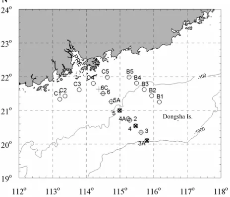
The NSCS was surveyed during two cruises (14 to 25 May 2001 and 2 to 21 November 2002) on board R/V Yanping II. Figure 1 shows the stations for CTD surveys and ab-15

sorption sampling. The 2001 cruise involved one transect (Transect A, hereafter T-A), starting from the vicinity of the PRE to the southeast to Dongsha island, and crossing the shelf to the slope. The 2002 cruise had two more transects: Transect B (here-after T-B) parallel to and to the east of T-A, and Transect C (here(here-after T-C) located outside the PRE, along the coast. Following Zhai et al. (2005), T-A can be divided into 20

two zones, inner shelf with water depths shallower than 100 m and within a range of ca. 75–130 km from the coast (Stas. 6C, 6 and 5A); and outer shelf/slope with water depths of 100–1000 m (Stas. 5, 4A, 2, 4, 3 and 3A).

Our May 2001 cruise was divided into two legs. The first cruise leg was between 14–19 May, and the second was during 24–25May. Stations 6 and 2 were sampled 25

in both cruise legs for absorption coefficients (the second sampling is annotated as Sta. 6’ and Sta. 2’, respectively).

BGD

Full Screen / Esc

Printer-friendly Version

Interactive Discussion

Our sample collection and measurements strictly followed the Ocean Optics Proto-cols Version 2.0, distributed by NASA (Mitchell et al., 2000). Briefly, water samples were collected with 1.7 L Niskin bottles mounted on a rosette equipped with a SBE19 CTD which provides temperature and salinity data. Samples were then filtered onto a 25-mm 0.7µm glass fiber filter (Whatman GF/F) under low vacuum (<17 kPa).

Sam-5

ple filters were put into tissue capsules (Fisher HistoprepT M) and then stored in liquid nitrogen for subsequent laboratory analysis at Xiamen University.

Absorption was measured on a dual-beam Varian Cary-100 spectrophotometer loaded with an integrating sphere. Sample filters were first scanned from 250 to 800 nm relative to a blank filter saturated with 0.2µm filtered seawater to obtain the total

par-10

ticulate absorbance spectra (OD_p). After pigment extraction with methanol, sample filters were measured again to obtain the absorbance spectra of the nonalgal particles (OD_d). OD_p(440) and OD_d(440) were all less than 0.4 absorbance.

Absorption coefficients of total particles (αp) and nonalgal particles (αd) were calcu-lated as:

15

α(λ) = 2.303 × [OD(λ) − ODnull]×

A V β,

where A is the area of the sample filter with concentrated particles, V is the volume of water filtered andβ is a parameter to correct for the pathlength amplification effect due

to multiple scattering. A widely acceptedβ expression given by Cleveland and

Wei-demann (1993) was used for correction. OD_null is the average of the OD between 790 20

and 800 nm since it had been found that all aquatic particles generally show negligible absorption in the near infrared. Phytoplankton absorption coefficients (αph) were then calculated as the difference between αpandαd.

The absorption of water samples from depths>150 m was too weak to detect, and

so only data for the upper 150 m of water are presented. 25

BGD

Full Screen / Esc

Printer-friendly Version

Interactive Discussion

3 Results and discussion

3.1 Variations ofα_phmagnitude and spectral shapes 3.2 Short term variation in May 2001

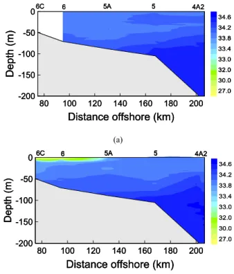
The outburst of SCS summer monsoon normally occurs in mid-May, leading to a rainy season (Qian et al., 2002). This was also the case in May 2001. Heavy precipitation 5

appeared on 1 May, 7–9 May, 17–18 May, and 21–22 May, recorded at both Baiyun (Guangzhou) and Hong Kong weather observatories as described in a parallel study (Dai et al., 2007). Accumulation of this precipitation caused a river plume extending to the region near Sta. 6 as evidenced by low salinity between 24 to 25 May (Fig. 2). Surface water salinity sharply dropped from 34.0 to∼26.5 at Sta. 6. The plume, which 10

apparently diminished at Sta. 5A, brought a significant amount of nutrients into the region shoreward of Sta. 5A, resulting in a phytoplankton bloom, as revealed by a parallel study on the carbonate system in this region (Dai et al., 2007).

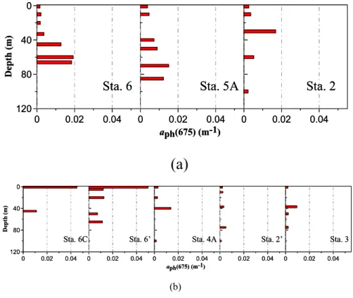
Correspondingly, the absorption properties experienced significant changes during this period of observation. Figure 3 shows vertical profiles ofα_ph(675) observed on T-A 15

in May 2001. During the first cruise leg between 15 and 19 May, the surfaceα_ph(675) varied from 0.002 m−1 at Sta. 6 to 0.004 m−1 at Sta. 5A (∼37 km apart) on the inner shelf, and no significant changes were found between the inner shelf and the outer shelf/slope. A subsurface maximum in α_ph(675) existed both on the inner shelf and the outer shelf/slope, with value varying between 0.015–0.019 m−1. During the second 20

cruise leg between 24–25 May, however, the horizontal gradient ofα_ph(675) increased substantially. On the inner shelf, the surfaceα_ph(675) became one order of magnitude higher than that on the outer shelf/slope. αph(675) as high as 0.050 m−1 occurred at Sta. 6. This was equivalent to an increase of chlα from 0.1 to 2.6 mg m−3 using the model of Carder et al. (1999) ([chlα] =56.8×[αph(675)]

1.03

), which was consistent with 25

BGD

Full Screen / Esc

Printer-friendly Version

Interactive Discussion

The occurrence of a phytoplankton bloom around Sta. 6 was thus evident. In contrast, the outer shelf/slope maintained a low surfaceαph(675) around 0.002 m−1 and a sub-surface/deep maximum varying between 0.005–0.014 m−1. For the two stations we revisited, significant changes were solely found at Sta. 6, where surface αph(675) in-creased from 0.002 to 0.050 m−1.

5

B/R ratios on the inner shelf also showed significant changes (Table 1). During the first cruise leg, the surface B/R ratios, both on the inner shelf and on the outer shelf/slope, were greater than 3.0. This implies the predominance of picoprocaryotes in the phytoplankton community (Stramski and Morel, 1990; Partensky et al., 1993; Moore et al., 1995). However, during the second leg, surface B/R ratio at Sta. 6 10

dropped from 3.9 to 2.5, suggesting a decrease in the proportion of picoprocaryotes in the phytoplankton community. This can be confirmed by the finding in the parallel car-bonate system study, which demonstrated that the phytoplankton community structure in terms of size-fractionated chlα significantly shifted from a pico/nano-phytoplankton

dominated community to a structure dominated by micro-algae in surface water at 15

Sta. 6 during the second cruise leg (Dai et al., 2007). Moreover, the shape of the

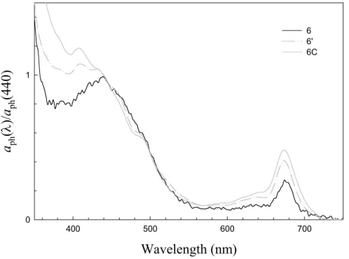
αph spectrum changed substantially (Fig. 4). Strong absorptions were found at 636 and 485 nm, suggesting abundance of chlc and fucoxanthin, typically contained in

di-atoms (Bidigare et al., 1990). The absorption maximum in the blue region shifted from 440 to 432 and 410 nm, indicating increasing levels of phaeopigments (Lorenzen and 20

Downs, 1986). It is thus suggestible that a diatom bloom at its late stage occurred around Sta. 6 when the second cruise leg took place. It should be noted that similar features in theαphspectra were observed at Sta. 6C (shoreward of Sta. 6, Fig. 4) with a B/R ratio as low as 2.1. On the outer shelf/slope, however, B/R ratios remained greater than 3.0 throughout the cruise.

BGD

Full Screen / Esc

Printer-friendly Version

Interactive Discussion

3.2.1 Seasonal variation in the outer shelf on Transect A

The inner shelf water on T-A was clearly subject to significant short term variations in May (a high flow season of the PRE). Comparisons ofαphbetween May and November, southwest and northeast monsoon seasons, will thus focus on the outer shelf/slope of T-A.

5

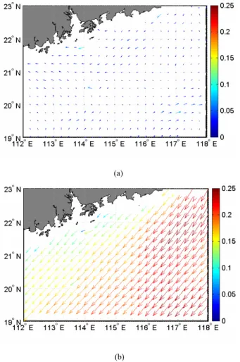
On average, the transition from the northeast to southwest monsoon in the SCS occurs in May and that from the southwest to the northeast occurs in October (Lau et al., 1998). Figure 5 displays the monthly mean distribution of QuikSCAT wind stress in the region under study in May 2001 and November 2002. The maximum northeasterly wind stress in November 2002 could be up to 0.25 N m−2. The wind stress in May 10

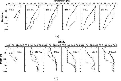
2001 was much smaller (mostly<0.1 N m−2) and variable in direction. The effect of wind forcing superimposed on surface cooling convective overturn in the northeast monsoon season would lead to enhanced vertical mixing, resulting in a deepening of mixed layer depth (MLD). Deepening of MLD in the region of interest in November 2002 as compared to May 2001 was obvious (Fig. 6). Except for Sta. 5, which was located 15

at 100 m isobath, MLD on the outer shelf/slope of T-A varied between 60–100 m in November, while it was less than 20 m in May. This suggests that the nutrients in the upper nutricline are more readily for primary production, leading to elevated chlα and

primary productivity, as had observed at a SCS time series station (SEATS) located in the NSCS (Tseng et al., 2005).

20

Concomitantly, both the surface value and the vertical structure ofα_ph(675) on the outer shelf/ slope of T-A in November 2002 differed from that in May 2001 (Fig. 7). For example, surfaceα_ph(675) along T-A varied from 0.005 to 0.009 m−1 in November, higher by 0.002–0.006 m−1 than those observed at the same stations in May 2001. Although subsurface maxima also existed in November, they were far less prominent 25

than those in May. The differences between the subsurface maxima and the surface values were typically less than 0.003 m−1 in November for most stations, whereas in May they were higher by at least a factor of two as compared to the November values.

BGD

Full Screen / Esc

Printer-friendly Version

Interactive Discussion

On the outer shelf of T-A, B/R ratios were generally greater than 3.0 in the upper water in both seasons, although the values were slightly higher in May than in Novem-ber (Table 2). Below the surface, B/R ratios at most of the sampling stations were less than 2.5 in November but greater than 2.5 in May. Difference between these two seasons may be primarily a result of photoacclimation since higher light condition is 5

usually observed in May.

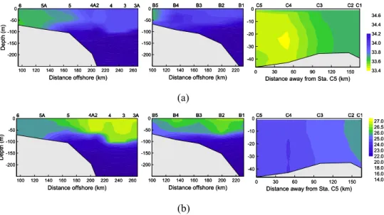
3.2.2 Spatial variation in November 2002

The survey of November 2002 covered a broader regions, T-B and T-C, in addition to T-A. Figure 8 displays their different hydrological properties. T-C was within ∼50 km distance from the coast, highly impacted by YueDong Coastal Water. This water mass, 10

low in salinity, is rich in nutrients and thus maintains a relatively high level of chlα and

primary productivity (Li and Su, 2001). T-B and T-A were on the shelf. T-B was located east of the PRE. Since the Pearl River plume went southwestward under the forcing of the northeast monsoon in November (Su, 2004), T-B was beyond the impact of the Pearl River plume. T-A, on the contrary, was right outside the PRE. Nutrient loadings 15

from the river plume to T-A was thus expected. On the other hand, it was suggested that vertical turbulence might have been reinforced on T-A due to the input of the Pearl River plume (Mann and Lazier, 1996), leading to a deeper MLD on T-A than on T-B (Fig. 8). This implies that nutrients might be more available for phytoplankton growth in the upper layer on T-A.

20

Corresponding to the different physical regimes, a clear spatial pattern of αph(675) appeared. As Fig. 9 shows, surfaceα_ph(675) was much higher on T-C than that on T-A and T-B. It ranged between 0.010–0.018 m−1 on T-C, corresponding to a range of

chl α between 0.49–0.91 mg m−3 according to the algorithm of Carder et al. (1999).

The highest value occurred at Sta. C4, which was located facing and closest to the 25

PRE, demonstrating that the Pearl River plume in this low flow season could still be influential to the area around 21.8◦N (see Fig. 1 for the location). There was no distinct

BGD

Full Screen / Esc

Printer-friendly Version

Interactive Discussion

subsurface/deep maximum inαph(675) on T-C, althoughαph(675) was slightly higher in deeper water than at the surface.

Surface α_ph(675) of T-B was relatively low compared to that of T-A, either on the inner shelf or on the outer shelf/slope. It was nearly homogenous, staying around 0.005 m−1 over the entire T-B. In contrast, it had a greater horizontal gradient along 5

T-A, varying between a minimum of 0.005 m−1on the outer shelf/slope and a maximum of 0.015 m−1 on the inner shelf. Vertical structures ofα_ph(675) were also different. A prominent subsurfaceαph(675) maximum was present on T-B, with a maximum level of 0.021 m−1, especially on the outer shelf/slope. For T-A, although a subsurfaceα_ph(675) maximum was visible, the values were lower. These variations ofαph(675) between two 10

shelf transects, T-A and T-B, partly proved that the Pearl River plume affected the inner shelf of T-A by supplying more nutrients for phytoplankton growth, either through direct input or by enhancing vertical mixing.

B/R ratios also changed among the three transects (Table 1). Generally, T-C had the lowest value (<2.5 for most stations) and T-B had the highest (>2.5 for most

sta-15

tions) (Table 1). On T-A, B/R ratios were higher on the outer shelf/slope than on the inner shelf, especially surface B/R ratios were close to or greater than 3.0 on the outer shelf/slope. Typical eukaryotic phytoplankton studied in the laboratory has not been observed with peak B/R ratios in excess of 2.5 (Cleveland et al., 1989), while pico-prokaryotes can exhibit B/R ratios much greater than that (Stramski and Morel, 1990; 20

Partensky et al., 1993; Moore et al., 1995). It seems that picoprocaryotes dominated on T-B and the outer shelf/slope of T-A, while this was not the case for T-C and the inner shelf of T-A, where the impact of Pearl River plume and coastal water might be severe. Another evidence was bathochromic shifts phenomena especially for Prochlorococcus. Bathochromic shifts from 440 nm were observed in the entire water column of T-B and 25

on the outer shelf of T-A in November (Fig. 10a). Such a shift increased in intensity from 4–6 nm to 40 nm in the deeper water while approaching the slope (Fig. 10b). Bathochromic shifts of∼7 nm, consistent with the presence of Prochlorococcus, were found in the deep layer of the Sargasso Sea (Bricaud and Stramski, 1990). A

simi-BGD

Full Screen / Esc

Printer-friendly Version

Interactive Discussion

larly strong shift of∼40 nm has been observed in the tropical North Atlantic (Lazzara et al., 1996). The shifts we encountered in November strongly suggested the pres-ence of Prochlorococcus in this season. This is partly supported by a parallel study on phytoplankton community structure on T-A based on HPLC pigment analysis (Chen et al., 2006). It was revealed that diatom dominated in the Pearl River Estuary and 5

the adjacent coastal area. However, the proportion of Prymnesiophyta, cyanobacte-ria and Prochlorococcus were main groups in the offshore water. The contribution of cyanobacteria and Prochlorococcus to chlα was 16–33% and 14–26% respectively on

the outer shelf (Sta. 5 was marked as SCS04 in Chen et al., 2006). 3.3 Variations in the absorption spectral model parameters 10

Among the SEADAS list of MODIS Level 3 products, there are absorption and backscatter coefficients derived from Carder et al. (1999) and QAA (Lee et al., 2002). Carder et al. (1999) chose a hyperbolic tangent function to model the relationship be-tweenα_ph(λ) versus α_ph(675) for high-light subtropical regimes as follows:

α_ph(λ) = a0 × exp(a1 × tanh(a2 × ln(αph(675)/a3))) × αph(675). 15

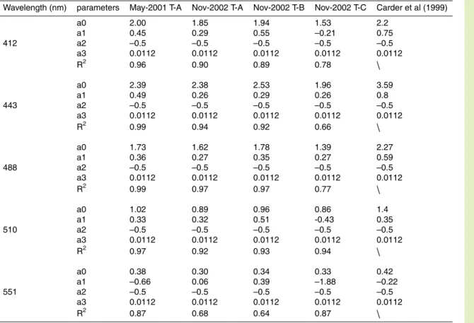
Table 2 show the NSCS regional tuning results of the Carder model for the MODIS wave bands centered atλ = 412, 443, 488, 510, 531 and 551 nm. Parameters a2 and

a3 were set to the same values proposed by Carder et al. (1999).

For T-A, there appeared to be minor variation of the model parameters between the two seasons (Table 2). The lead parameter a0 was slightly higher in May 2001 20

than in November 2002. The largest difference between them occurred at 551 nm, corresponding to a change of∼30%. Variations of a0 at the other bands were <10%.

Differences of the model parameters between the coastal transect T-C and the shelf transects T-A and T-B in November 2002 were relatively significant (Table 2). For the three bands 412, 443 and 488 nm, the lead parameter, a0, was about 20% lower on 25

BGD

Full Screen / Esc

Printer-friendly Version

Interactive Discussion

It is thus suggested that a regional tuning (i.e., from the coastal water adjacent to the PRE to the NSCS shelf water) may be important for semi-analytical model parameter-ization. Tuning between the two seasons under study seems less important although a full seasonal cycle of the absorption spectral model is desirable. In addition, the pa-rameters in this region deviated from those originally proposed in Carder et al. (1999), 5

further demonstrating that a single parameterization is not applicable globally, and re-gional tuning is often required.

4 Summary

Variability of the phytoplankton absorption coefficients (αph) in the northern South China Sea (NSCS) adjacent to the Pearl River estuary (PRE) was examined based 10

upon two cruise surveys (May 2001 and November 2002). Significant temporal and spatial variations of α_ph(675) have been found. Short-term variability in May 2001 revealed the influence of a phytoplankton bloom downstream of a large river plume induced by heavy precipitation. Seasonal differences indicated the deeper mixing in November 2002 due to the stronger winter monsoon. Becauseα_ph(675) is highly cor-15

related with chlα, these variations of α_ph(675) are expected to reflect the pattern of

chlα, knowledge of which is still rather limited in this region. Furthermore, variations

in the absorption characteristics, such as blue/red (B/R) ratio and bathochromic shift, inferred change of phytoplankton community structure. For example, picoprocaryotes were probably an important component of the phytoplankton community on the outer 20

shelf/slope of T-A in November, while this seemed not the case for its inner shelf por-tion, where the impact of Pearl River plume and coastal water was high. The results here show the potential of applyingαph, a parameter relatively easy to determine, to obtain some information about the phytoplankton standing stock and community struc-ture. In addition, fitting the measured data to the spectral model of α_ph of Carder et 25

al. (1999) found greater spatial variations than seasonal variations in the model param-eters, suggesting that separate models or parameters for coastal and shelf waters are

BGD

Full Screen / Esc

Printer-friendly Version

Interactive Discussion

required in order to accurately deriveα_phremotely for developing local semi-analytical algorithms.

The NSCS is a complex water body subject to local river plumes and coastal waters modulated by monsoon and other factors. Therefore, the limited data obtained from the two cruises are insufficient to provide the full scenario of temporal (event to non-event, 5

seasonal) and spatial (shelf to slope) variability ofα_phin this water, and more intensive investigation is required. Nevertheless, our results provide for the first time a sketch of the spatial and temporal variations ofαphassociated with physical processes in this region.

Acknowledgements. This work was supported by the Natural Science Foundation of China 10

through grants #40376031, # 90211020 and #40521003, and by the Ministry of Science and Technology of China through #2002AA639540. This work is also partially supported by the Pro-gram for Changjiang Scholars and Innovative Research Team in University, and the ProPro-gram for New Century Excellent Talents in University (Xiamen University). The QuikSCAT wind data were obtained from the Physical Oceanography Distributed Active Archive Center (PO.DAAC)

15

at the NASA Jet Propulsion Laboratory, Pasadena, CA (http://podaac.jpl.nasa.gov). We thank C. Hu of the South Florida University for his detailed and constructive comments and sugges-tions. We are grateful to the crew of the R/V Yanping II, Z. Chen and D. Chen for collecting the hydrographic data and processing wind stress data. We also thank J. Hodgkiss for editing the manuscript.

20

References

Babin, M., Stramski, D., Ferrari, G. M., Claustre, H., Bricaud, A., Obolensky, G., and Hoepffner, N.: Variations in the light absorption coefficients of phytoplankton, nonalgal particles, and dissolved organic matter in coastal waters around Europe, J. Geophys. Res., 108(C7), 3211, doi:10.1029/2001JC000882, 2003.

25

Bidigare, R. R., Ondrusek, M. E., Morrow, J. H., and Kiefer, D. A.: In vivo absorption properties of algal pigments, Proc. SPIE Ocean Opt. X, 1302, 290–302, 1990.

BGD

Full Screen / Esc

Printer-friendly Version

Interactive Discussion from measurements of spectral irradiance and pigment concentrations, Global Biogeochem.

Cycles, 1, 171–186, 1987.

Bricaud, A. and Stamski, D.: Spectral absorption coefficients of living phytoplankton and non-algal biogenous matter: A comparison between the Peru upwelling area and the Sargasso Sea, Limnol. Oceanogr., 35(3), 562–582, 1990.

5

Bukata, R. P., Jerome, J. H., Kondratyev, K. Y., and Pozdnyakov, D. V.: Optical properties and remote sensing of inland and coastal waters, CRC Press, Boca Raton, FL, 1995.

Cai, W. J. and Dai, M.: Comment on “Enhanced open ocean storage of CO2 from shelf sea pumping”, Science, 306, 1477C, 2004.

Cao, W. X., Yang, Y. Z., Xu, X. Q., Huang, L. M., and Zhang, J. L.: Regional patterns of

10

particulate spectral absorption in the Pearl River estuary, Chinese Science Bulletin, 48(21), 2344–2351, 2003.

Cao, W., Yang, Y., Liu, S., Xu, X., Yang, D., and Zhang, J.: Spectral absorption coefficients of phytoplankton in relation to chlorophyll a and remote sensing reflectance in coastal waters of southern China, Progress in Natural Science, 15(4), 342–350, 2005 (in Chinese with English

15

abstract).

Carder, K. L., Chen, F. R., Lee, Z. P., and Hawes, S. K.: Semianalytic Moderate-Resolution Imaging Spectrometer algorithms for chlorophyll and absorption with bio-optical domains based on nitrate-depletion temperatures, J. Geophys. Res., 104, 5403–5421, 1999.

Chen, J. X., Huang, B. Q., Liu, Y., Cao, Z. R., and Hong, H. S.: Phytoplankton community

20

structure in the transects across East China Sea and Northern South China Sea determined by analysis of HPLC photosynthetic pigment signatures, Advances in Earth Science, 21(7), 738–746, 2006 (in Chinese with English abstract).

Chisholm, S. W., Olson, R. J., Zettler, E. R., Goericke, R., Waterbury, J. B., and Welschmeyer, N. A.: A novel free-living prochlorphyte abundant in the oceanic euphotic zone, Nature, 334,

25

340–343, 1988.

Cleveland, J. S.: Regional models for phytoplankton absorption as a function of chlorophyll a concentration, J. Geophys. Res., 100(C7), 13 333–13 344, 1995.

Cleveland, J. S., Perry, M. J., Kiefer, D. A., and Talbot, M. C.: Maximal quantum yield of photo-synthesis in the northwestern Sargasso Sea, J. Mar. Res., 47, 869–886, 1989.

30

Cleveland, J. S. and Weidemann, A. D.: Quantifying absorption by aquatic particles: A multiple scattering correction for glass-fiber filters, Limnol. Oceanogr., 38, 1321–1327, 1993.

BGD

Full Screen / Esc

Printer-friendly Version

Interactive Discussion Lu, Z., Chen, W., and Chen, Z.: Effects of an estuarine plume-associated bloom on the

carbonate system in the lower reaches of the Pearl River estuary and the coastal zone of the northern South China Sea, Cont. Shelf Res., accepted, 2007.

Huang, B. Q., Lin, X. J., Liu, Y., Dai, M. H., Hong, H. S., and Li, W. K. K.: Ecological study of picoplankton in northern South China Sea, Chinese J. Oceanol. Limnol., 20, 22–32, 2002.

5

IOCCG: Remote sensing of ocean colour in coastal, and other optically-complex, waters: Re-port of the International Ocean Color Coordinating Group, No.3, edited by: Sathyendranath, S., IOCCG, Dartmouth, Nova Scotia Canada, 140 pp, 2000.

Kana, T. M., Glibert, P. M., Goericke, R., and Welschmeyer, N. A.: Zeaxanthin andβ-carotene in

Synechococcus WH7803 respond differently to irradiance, Limnol. Oceanogr., 33(6), 1623–

10

1627, 1988.

Lau, K. M., Wu, H. T., and Yang, S.: Hydrologic processes associated with the first transition of the Asian summer monsoon : a pilot satellite study, Bull. Am. Meteorol. Soc., 79, 1871–1882, 1998.

Lazzara, L., Bricaud, A., and Claustre, H.: Spectral absorption and fluorescence excitation

15

properties of phytoplanktonic populations at a mesotrophic and an oligotrophic site in the tropical North Atlantic (EUMELI program), Deep Sea Res. I, 43(8), 1215–1240, 1996. Lee Chen, Y.: Spatial and seasonal variations of nitrate-based new production and primary

production in the South China Sea, Deep Sea Res. I, 52, 319–340, 2005.

Lee, Z. P., Carder, K. L., and Arnone, R.: Deriving inherent optical properties from water color:

20

a multi-band quasi-analytical algorithm for optically deep waters, Appl. Opt., 41, 5755–5772, 2002.

Lee, Z. P., Carder, K. L., Steward, R. G., Peacock, T. G., Davis, C. O., and Patch, J. S.: An empirical algorithm for light absorption by ocean water based on color, J. Geophys. Res., 103(C12), 27 967–27 978, 1998.

25

Li, F. Q. and Su, Y. S.: Analysis of water masses, Qingdao ocean university press, 375–385, 2001.

Liu, K. K., Chao, S. Y., Shaw, P. T., Gong, G. C., Chen, C. C., and Tang, T. Y.: Monsoon-forced chlorophyll distribution and primary production in the South China Sea: Observations and a numerical study, Deep Sea Res. I, 49, 1387–1412, 2002.

30

Lorenzen, C. J. and Downs, J. N.: The specific absorption coefficients of chlorophyllide a and pheophorbide a in 90% acetone, and comments on the fluorometric determination of chloro-phyll and pheopigments, Limnol.Oceanogr., 31(2), 449–452, 1986.

BGD

Full Screen / Esc

Printer-friendly Version

Interactive Discussion Lohrenz, S., Weidemann, A. D., and Tuel, M.: Phytoplankton spectral absorption as influenced

by community size structure and pigment composition, J. Plankton Res., 25(1), 35–61, 2003. Lutz, V. A., Sathyendranath, S., and Head, E. J. H.: Absorption coefficient of phytoplankton:

regional variations in the North Atlantic, Mar. Ecol. Prog. Ser., 135, 197–213, 1996.

Mann, K. H. and Lazier, J. R. N.: Dynamics of marine ecosystems, Blackwell Science, 389 pp,

5

1996.

Mitchell, B. G., Bricaud, A., Carder, K., Cleveland, J., Ferrari, G. M., Gould, R., Kahru, M., Kishino, M., Maske, H., Moisan, T., Moore, L., Nelson, N., Phinney, D., Reynolds, R. A., Sosik, H., Stramski, D., Tassan, S., Trees, C., Weidemann, A., Wieland, J. D., and Vodacek, A.: Determination of spectral absorption coefficients of particles, dissolved material and

10

phytoplankton for discrete water samples, in Ocean Optics Protocols for Satellite Ocean Color Sensor Validation, Revision 2, edited by: Fargion, G. S., Mueller, J. L., and McClain, C. R., NASA, Goddard space flight center, Greenbelt, Maryland, 125–153, 2000.

Mitchell, B. G. and Kiefer, D. A.: Chlorophyll a specific absorption and fluorescence excitation spectra for light limited phytoplankton, Deep Sea Res., 35(5), 639–663, 1988.

15

Moore, L. R., Goericke, R., and Chisholm, S. W.: Comparative physiology of Synechococcus and Prochlorococcus: influence of light and temperature on growth, pigments, fluorescence and absorptive properties, Mar. Ecol. Prog. Ser., 116, 259–275, 1995.

Morel, A., Antoine, D., Babin, M., and Dandonneau, Y.: Measured and modeled primary pro-duction in the northeast Atlantic (EUMELI JOGFS program): the impact of natural variations

20

in the photosynthetic parameters on model predictive skill, Deep Sea Res. I, 43(8), 1273– 1304, 1996.

Ning, X., Chai, F., Xue, H., Cai, Y., Liu, C., and Shi, J.: Physical-biological oceanographic cou-pling influencing phytoplankton and primary production in the South China Sea, J. Geophys. Res., 109, C10005, doi:10.1029/2004JC002365, 2004.

25

Ning, X. R., Cai, Y. M., Li, G. W., and Shi, J. X.: Photosynthetic picoplankton in the northern South China Sea, Acta Oceanologica Sinica, 25(3), 83–97, 2003 (in Chinese with English abstract).

Partensky, F., Hoepffner, N., Li, W. K. W., Ulloa, O., and Vaulot, D.: Photoacclimation of

Prochlorococcus sp. (Prochlorophyta) strains isolated from North Atlantic and the Mediter-30

ranean Sea, Plant Physiol., 101, 285–296, 1993.

Preisendorfer, R. W.: Application of radiative transfer theory to light measurements in the sea, International Union of Geodesy and Geophysics, 11–30, 1961.

BGD

Full Screen / Esc

Printer-friendly Version

Interactive Discussion Prieur, L. and Sathyendranath, S.: An optical classification of coastal and oceanic waters based

on the specific spectral absorption curves of phytoplankton pigments, dissolved organic mat-ter, and other particulate materials, Limnol. Oceanogr., 26, 671–689, 1981.

Qian, W. H., Zhu, Y. F., Kang, H. S, and Lee, D. K.: Temporal-spatial distribution of seasonal rainfall and circulation in the East Asian monsoon region, Theoretical and Applied

Climatol-5

ogy, 73, 151–168, 2002.

Sosik, H. M. and Mitchell, B. G.: Absorption, fluorescence and quantum yield for growth in nitrogen-limited Dunaliella tertiolecta, Limnol. Oceanogr., 36, 910–921, 1991.

Stramski, D. and Morel, A.: Optical properties of photosynthetic picoplankton in different physi-ological states as affected by growth irradiance. Deep Sea Res., 37, 245–266, 1990.

10

Stuart, V., Sathyendranath, S., Platt, T., Maass, H., and Irwin, B.: Pigments and species com-position of natural phytoplankton populations: effect on the absorption spectra, J. Plankton Res., 20, 187–217, 1998.

Su, J.: Overview of the South China Sea circulation and its influence on the coastal physical oceanography outside the Pearl River Estuary, Cont. Shelf Res., 24, 1745–1760, 2004.

15

Tseng, C. M., Wong, G. T. F., Lin, I. I., Wu, C. R., and Liu, K. K.: A unique seasonal pattern in phytoplankton biomass in low-latitude waters in the South China Sea, Geophys. Res. Lett., 32, L08608, doi:10.1029/2004GL022111, 2005.

Wang, G. F., Cao, W. X., Xu, D. Z., Liu, S., and Zhang, J. L.: Variations in specific absorption coefficients of phytoplankton in northern South China Sea, J. tropical Oceanogr., 24(5), 1–

20

10, 2005 (in Chinese with English abstract).

Xu, X. Q., Cao, W. X., and Yang, Y. Z.: Relationships between spectral absorption coefficient of particulates and salinity and chlorophyll a concentration in Zhujiang river mouth, J. Tropical Oceanogr., 23(5), 63–71, 2004(in Chinese with English abstract).

Zhai, W. D., Dai, M. H., Cai, W. J., Wang, Y. C., and Hong, H. S.: The partial pressure of carbon

25

dioxide and air–sea fluxes in the northern South China Sea in spring, summer and autumn, Mar. Chem., 96, 87–97, 2005.

Zhu, G., Ning, N., Cai, Y., Liu, Z., and Liu, Z.: Studies on species composition and abundance distribution of phytoplankton in the South China Sea, Acta Oceanologica Sinica, 25(supp.2), 8–23, 2003 (in Chinese with English abstract).

BGD

Full Screen / Esc

Printer-friendly Version

Interactive Discussion

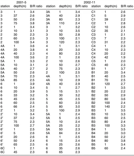
Table 1. B/R ratios (α_ph(440)/α_ph(675)) in the Northern South China Sea in May 2001 and November 2002.

2001-5 2002-11

station depth(m) B/R ratio station depth(m) B/R ratio station depth(m) B/R ratio

3 1 3.4 3A 1 3.4 C1 1 2.6 3 37 2.6 3A 40 2.9 C1 5 2.9 3 50 2.6 3A 80 2.3 C1 39 2.2 3 75 3.8 3A 110 2.4 C2 1 2.8 2 1 3.4 3 1 3.2 C2 10 2.6 2 10 3.1 3 10 3.5 C2 35 2.1 2 30 2.3 3 50 2.8 C3 1 2.1 2 60 2.5 3 100 2.1 C3 7 2.3 2 100 3.4 3 120 2.3 C3 31 2.2 4A 1 3.6 4 1 3.1 C4 1 2.3 4A 20 3.8 4 20 3.0 C4 10 2.3 4A 40 2.3 4 80 2.3 C4 20 2.2 4A 100 3.6 2 1 2.6 C4 42 1.9 5A 1 3.3 2 10 2.6 C5 1 2.0 5A 10 3.1 2 50 2.7 C5 40 2.3 5A 40 2.7 2 75 2.3 B1 1 3.7 5A 50 2.6 2 100 2.5 B1 20 3.4 5A 70 2.3 4A 1 3.1 B1 40 2.5 5A 85 2.5 4A 10 2.9 B1 70 2.5 6 1 3.9 4A 40 2.9 B1 120 2.7 6 10 3.4 5 1 2.7 B2 1 3.5 6 20 3.9 5 15 3.1 B2 20 2.2 6 33 3.2 5 30 3.2 B2 50 2.9 6 45 2.6 5 45 2.5 B2 80 3.6 6 60 2.5 5 60 2.0 B2 100 2.4 6 66 2.4 5 80 3.0 B2 140 2.2 2’ 1 3.2 5 100 2.9 B3 1 3.5 2’ 10 3.4 5A 1 2.4 B3 10 3.3 2’ 37 3.2 5A 5 2.5 B3 60 2.5 2’ 75 2.3 5A 10 2.4 B3 80 2.4 2’ 100 2.7 5A 25 2.2 B3 100 3.3 6’ 1 2.5 5A 50 2.3 B4 1 3.5 6’ 5 2.6 5A 84 2.4 B4 20 3.0 6’ 20 2.6 6 1 2.5 B4 50 2.2 6’ 50 2.4 6 15 2.4 B4 80 3.8 6’ 65 2.5 6 25 2.6 B5 1 3.4 6C 1 2.1 6 35 2.6 B5 60 2.4 6C 45 2.3 6 65 2.3

BGD

Full Screen / Esc

Printer-friendly Version

Interactive Discussion

Table 2. Parameters of the phytoplankton absorption spectral model.

Wavelength (nm) parameters May-2001 T-A Nov-2002 T-A Nov-2002 T-B Nov-2002 T-C Carder et al (1999)

a0 2.00 1.85 1.94 1.53 2.2 a1 0.45 0.29 0.55 –0.21 0.75 412 a2 –0.5 –0.5 –0.5 –0.5 –0.5 a3 0.0112 0.0112 0.0112 0.0112 0.0112 R2 0.96 0.90 0.89 0.78 \ a0 2.39 2.38 2.53 1.96 3.59 a1 0.49 0.26 0.29 0.26 0.8 443 a2 –0.5 –0.5 –0.5 –0.5 –0.5 a3 0.0112 0.0112 0.0112 0.0112 0.0112 R2 0.99 0.94 0.92 0.66 \ a0 1.73 1.62 1.78 1.39 2.27 a1 0.36 0.27 0.35 0.27 0.59 488 a2 –0.5 –0.5 –0.5 –0.5 –0.5 a3 0.0112 0.0112 0.0112 0.0112 0.0112 R2 0.99 0.97 0.97 0.77 \ a0 1.02 0.89 0.96 0.86 1.4 a1 0.33 0.32 0.51 -0.43 0.35 510 a2 –0.5 –0.5 –0.5 –0.5 –0.5 a3 0.0112 0.0112 0.0112 0.0112 0.0112 R2 0.97 0.92 0.93 0.94 \ a0 0.38 0.30 0.34 0.33 0.42 a1 –0.66 0.06 0.39 –1.88 –0.22 551 a2 –0.5 –0.5 –0.5 –0.5 –0.5 a3 0.0112 0.0112 0.0112 0.0112 0.0112 R2 0.87 0.68 0.64 0.87 \

BGD

Full Screen / Esc

Printer-friendly Version Interactive Discussion P R E -100 -1000 P R E -100 -1000 E N Dongsha Is. P R E -100 -1000 P R E -100 -1000 E N P R E -100 -1000 P R E -100 -1000 E N Dongsha Is.

Fig. 1. CTD and sampling stations in the northern South China Sea. +: CTD and sampling

stations in May 2001;×: stations only for CTD in May 2001; : CTD and sampling stations in November 2002; PRE: the Pearl River Estuary; Dongsha Is.: Dongsha island.

BGD

Full Screen / Esc

Printer-friendly Version Interactive Discussion 6C 6 5A 5 4A2 -200 -150 -100 -50 0 D e p th (m) 80 100 120 140 160 180 200 Distance offshore (km) 27.0 30.0 32.0 33.0 33.4 33.8 34.2 34.6 6C 6 5A 5 4A2 6C 6 5A 5 4A2 -200 -150 -100 -50 0 D e p th (m) 80 100 120 140 160 180 200 Distance offshore (km) 27.0 30.0 32.0 33.0 33.4 33.8 34.2 34.6 -200 -150 -100 -50 0 D e p th (m) 80 100 120 140 160 180 200 Distance offshore (km) 27.0 30.0 32.0 33.0 33.4 33.8 34.2 34.6 (a) -200 -150 -100 -50 0 D e p th (m) 80 100 120 140 160 180 200 Distance offshore (km) 6C 6 5A 5 4A2 27.0 30.0 32.0 33.0 33.4 33.8 34.2 34.6 -200 -150 -100 -50 0 D e p th (m) 80 100 120 140 160 180 200 Distance offshore (km) 6C 6 5A 5 4A2 -200 -150 -100 -50 0 D e p th (m) 80 100 120 140 160 180 200 Distance offshore (km) 6C 6 5A 5 4A2 6C 6 5A 5 4A2 27.0 30.0 32.0 33.0 33.4 33.8 34.2 34.6 (b) Fig. 2

BGD

Full Screen / Esc

Printer-friendly Version Interactive Discussion 120 80 40 0 D ep th (m) 0 0.02 0.04 0 0.02 0.04 aph(675) (m-1) 0 0.02 0.04

Sta. 6

Sta. 5A

Sta. 2

120 80 40 0 D ep th (m) 0 0.02 0.04 0 0.02 0.04 aph(675) (m-1) 0 0.02 0.04

Sta. 6

Sta. 5A

Sta. 2

(a)

Fig. 3

Sta. 6’ Sta. 4A Sta. 2’ Sta. 3

Sta. 6C 0 0.02 0.04 120 80 40 0 D ep th (m) 0 0.02 0.04 0 0.02 0.04 aph(675) (m-1) 0 0.02 0.04 0 0.02 0.04

Sta. 6’ Sta. 4A Sta. 2’ Sta. 3

Sta. 6C

(b)

Fig. 3. Vertical distribution ofα_ph(675) during the two cruise legs in May 2001. (a) 14–19 May;

BGD

Full Screen / Esc

Printer-friendly Version Interactive Discussion

Wavelength (nm)

a

(λ

)/

a

(440)

Fig. 4. Surfaceα_ph normalized at 440 nm at Sta. 6 and Sta. 6C. Sta. 6C was sampled during the second cruise leg when Sta. 6 was revisited (annotated as Sta. 6’).

BGD

Full Screen / Esc

Printer-friendly Version Interactive Discussion (a) Fig. 5 (b) Fig. 5

Fig. 5. Monthly mean wind stress as observed by QuikSCAT during May 2001 (a) and

BGD

Full Screen / Esc

Printer-friendly Version Interactive Discussion 14 18 22 26 30 160 120 80 40 0 D e p th ( m ) 14 18 22 26 30 14 18 22 26 30 Temperature (oC) 14 18 22 26 30 14 18 22 26 30 14 18 22 26 30

Sta. 5 Sta. 4A Sta. 2 Sta. 4 Sta. 3 Sta. 3A

14 18 22 26 30 160 120 80 40 0 D e p th ( m ) 14 18 22 26 30 14 18 22 26 30 Temperature (oC) 14 18 22 26 30 14 18 22 26 30 14 18 22 26 30

Sta. 5 Sta. 4A Sta. 2 Sta. 4 Sta. 3 Sta. 3A

(a) Fig. 6 33.6 34 34.4 34.8 160 120 80 40 0 D e p th ( m ) 33.6 34 34.4 34.8 33.6 34 34.4 34.8 Salinity 33.6 34 34.4 34.8 33.6 34 34.4 34.8 33.6 34 34.4 34.8

Sta. 5 Sta. 4A Sta. 2 Sta. 4 Sta. 3 Sta. 3A

33.6 34 34.4 34.8 160 120 80 40 0 D e p th ( m ) 33.6 34 34.4 34.8 33.6 34 34.4 34.8 Salinity 33.6 34 34.4 34.8 33.6 34 34.4 34.8 33.6 34 34.4 34.8

Sta. 5 Sta. 4A Sta. 2 Sta. 4 Sta. 3 Sta. 3A

(b)

Fig. 6

Fig. 6. Temperature (a) and salinity (b) profiles on the outer shelf/slope of transect A. The solid

BGD

Full Screen / Esc

Printer-friendly Version

Interactive Discussion

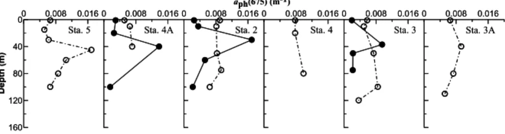
Sta. 5 Sta. 4A Sta. 2 Sta. 4 Sta. 3 Sta. 3A

0 0.008 0.016 160 120 80 40 0 D e p th (m ) 0 0.008 0.016 0 0.008 0.016 aph(675) (m-1) 0 0.008 0.016 0 0.008 0.016 0 0.008 0.016

Sta. 5 Sta. 4A Sta. 2 Sta. 4 Sta. 3 Sta. 3A

0 0.008 0.016 160 120 80 40 0 D e p th (m ) 0 0.008 0.016 0 0.008 0.016 aph(675) (m-1) 0 0.008 0.016 0 0.008 0.016 0 0.008 0.016

Fig. 7. Vertical distribution ofα_ph(675) on the outer shelf/slope of transect A. Observations in May 2001 and November 2002 are represented with bold and open circles respectively.

BGD

Full Screen / Esc

Printer-friendly Version Interactive Discussion 33.4 33.6 33.8 34.0 34.2 34.4 34.6 100 120 140 160 180 200 220 240 260 Distance offshore (km) -200 -150 -100 -50 0 D e p th (m) 100 120 140 160 180 200 220 Distance offshore (km) -200 -150 -100 -50 0 6 5A 5 4A2 4 3 3A B5 B4 B3 B2 B1 C5 C4 C3 C2 C1 0 30 60 90 120 150

Distance away from Sta. C5 (km)

-40 -30 -20 -10 0 33.4 33.6 33.8 34.0 34.2 34.4 34.6 100 120 140 160 180 200 220 240 260 Distance offshore (km) -200 -150 -100 -50 0 D e p th (m) 100 120 140 160 180 200 220 Distance offshore (km) -200 -150 -100 -50 0 6 5A 5 4A2 4 3 3A 6 5A 5 4A2 4 3 3A B5B5 B4B4 B3B3 B2B2 B1B1 C5C5 C4C4 C3C3 C2 C1C2 C1 0 30 60 90 120 150

Distance away from Sta. C5 (km)

-40 -30 -20 -10 0 (a) Fig. 8 14.0 16.0 18.0 20.0 22.0 23.0 24.0 25.0 26.0 26.5 27.0 100 120 140 160 180 200 220 240 260 Distance offshore (km) -200 -150 -100 -50 0 D e p th ( m ) 100 120 140 160 180 200 220 Distance offshore (km) -200 -150 -100 -50 0 0 30 60 90 120 150

Distance away from Sta. C5 (km)

-40 -30 -20 -10 0 6 5A 5 4A2 4 3 3A B5 B4 B3 B2 B1 C5 C4 C3 C2 C1 14.0 16.0 18.0 20.0 22.0 23.0 24.0 25.0 26.0 26.5 27.0 100 120 140 160 180 200 220 240 260 Distance offshore (km) -200 -150 -100 -50 0 D e p th ( m ) 100 120 140 160 180 200 220 Distance offshore (km) -200 -150 -100 -50 0 0 30 60 90 120 150

Distance away from Sta. C5 (km)

-40 -30 -20 -10 0 6 5A 5 4A2 4 3 3A 6 5A 5 4A2 4 3 3A B5B5 B4B4 B3B3 B2B2 B1B1 C5C5 C4C4 C3C3 C2 C1C2 C1 (b)

Fig. 8. Salinity (a) and temperature (b) distribution on Transect-A, B and C (from left to right) in

BGD

Full Screen / Esc

Printer-friendly Version Interactive Discussion a ph(675) (m -1 ) 0.000 .005 .010 .015 .020 .025 D ept h (m ) 0 20 40 60 80 100 120 140 6 5A 5 4A 2 4 3 3A (a) Fig. 9 a ph(675) (m -1 ) 0.000 .005 .010 .015 .020 .025 D ept h (m ) 0 20 40 60 80 100 120 140 B1 B2 B3 B4 B5 (b) Fig. 9 a ph(675) (m -1 ) 0.000 .005 .010 .015 .020 .025 D ept h (m ) 0 10 20 30 40 50 60 C1 C2 C3 C4 C5 (c) Fig. 9

BGD

Full Screen / Esc

Printer-friendly Version Interactive Discussion wavelength (nm) 400 500 600 700 aph (λ )/ aph (440) 0 1 6 5A 5 4A 2 4 3 3A (a) Fig. 10 wavelength (nm) 400 500 600 700 aph (λ )/ aph (4 40) 0 1 1 10 50 100 120 (b) Fig. 10

Fig. 10. α_phnormalized at 440 nm in November 2002. (a) Surface distribution on Transect A;

(b) Vertical distribution at Sta. 3. The legend in (b) shows the sampling depths in meters. The