Back to the city : differences in economic and investment performances between downtowns and suburbs

(1)

by Inae Hwang

B.Eng., Architectural Engineering, 2000 Yeungnam University, Korea M.S., Architectural Engineering, 2004

Seoul National University, Korea

Submitted to the Program in Real Estate Development in Conjunction with the Center for Real Estate in Partial Fulfillment of the Requirements for the Degree of

MASTER OF SCIENCE IN REAL ESTATE DEVELOPMENT at the

MASSACHUSETTS INSTITUTE OF TECHNOLOGY September, 2012

The author hereby grants to MIT permission to reproduce and to distribute publicly paper and electronic copies of this thesis document in whole or in part in any medium now known or hereafter created.

Signature of Author____________________________________________________________________ Center for Real Estate

July 30, 2012

Certified by___________________________________________________________________________ William C. Wheaton

Professor of Economics, Department of Economics Thesis Supervisor

Accepted by___________________________________________________________________________ David Geltner

Chair, MSRED Committee, Interdepartmental Degree Program in Real Estate Development

(2)

(3)

M.I.T. | ABSTRACT 3

Back to the City:

Differences in Economic and Investment Performances between Downtowns and Suburbs

by

Inae Hwang

Submitted to the Program in Real Estate Development in Conjunction with the Center for Real Estate on July 30, 2012 in Partial Fulfillment of the Requirements for the Degree of

Master of Science in Real Estate Development

ABSTRACT

Recently, we have observed significant changes in which corporate offices and residential buildings have been relocated from the suburbs back into the city. Does the observation mean that there is a real economic movement back into the cities by firms or households? If there is any movement, how does this trend drive any changes in the commercial real estate properties? Does it significantly affect the performance of properties in the cities as opposed to the other areas? Does the performance of the properties in the city exert any influence on the investors who prefer commercial real estates in the US metropolitan areas?

This thesis aims to provide answers to the major question on the “back to the city” movement and its influence on real estate markets. The answers are summarized as five major conclusions. First, the result of this study clearly points out that there is the “back to the city” movement although the change has happened only in the Urban Cores (UC) not the entire Metropolitan Statistical Area (MSA). Second, the economic performances between UC and MSA maintain a close link with each other. However, the volatility of the office net rental rate is much less in UC while the change in gross rental growth is almost same between UC and MSA. The UC rental growth of the multifamily is a little less volatile than the MSA growth. Third, the investment performances in MSA closely relates with the capitalization rate of UC. While the level of cap rates of UC offices is more volatile, the UC cap rate of apartments is more stable than the MSA rate. Fourth, the effects of population and employment on the real estate market enable the research to understand the current pricing behaviors. The difference in population and employment between UC and MSA explains the disparity in investment performances of the two areas. However, while the MSA rental growth explains the movements in the cap rate of MSA in accordance with the “rational” pricing, the effect of UC rental growth rates on the cap rate doesn’t match with the pricing model, indicating that the rental growth rate of UC empirically leads to increases in the cap rate of the area. The nature of these outcomes offers that the UC market is not explicable by the “rational” pricing model. The result also indicates that the difference in rental growth rates reveals the positive relation with the gap in cap rates, which is complete opposite to the “rational” investors’ behavior. Lastly, finding the differences in economic and investment performances between UC and MSA motivates to explore the determinants of the relationship. Although the study experiments the effects of manifold market characteristics, the explanatory variables used in the model do not fully explain the inequality between two specific markets. Thus, it is required to study further the determinants.

Thesis Supervisor: William C. Wheaton

(4)

(5)

M.I.T. | ACKNOWLEDGEMENT 5

ACKNOWLEDGEMENT

This thesis would be impossible without a number of generous and great people who supported me in the whole class year. I would like to extend my sincere appreciation to my thesis advisor, Professor Bill Wheaton for giving the constructive and clear guidance on developing the ideas and figuring out the fascinating topic. Also, I would like to thank Ann Ferracane at CBRE EA for providing the support and access to data sources in this thesis. I also thank Schery Bokhari and Chunil Kim for sharing their knowledge in data processing.

I would like to thank my classmates, the MIT faculty and staff, and MIT CRE alumni for making my first oversea educational experience valuable and memorable. I will miss so much the time when we learn, laugh, and live together. I feel very lucky because I have lifetime friends like you.

The special thank goes to all of my friends and family who always trust and take care of me. I would not be here without their love and support.

(6)

(7)

M.I.T. | TABLE OF CONTENTS 7

TABLE OF FIGURES

[Figure 1] Thesis Framework ... 16

[Figure 2] Zone Definition ... 22

[Figure 3] Defined Zones in Boston ... 23

[Figure 4] Population Growth Rates ... 30

[Figure 5] Comparison of Growth Rates ... 30

[Figure 6] Average of the MSA Population Growth Rate in 52 Metropolitan Areas from 1990 to 2010 .. 31

[Figure 7] Average of the UC Population Growth Rate in 52 Metropolitan Areas from 1990 to 2010 ... 32

[Figure 8] Average of the Population Growth Rate between UC and MSA in 2000 ... 33

[Figure 9] Average of the Population Growth Rate between UC and MSA in 2010 ... 33

[Figure 10] Employment Growth Rates ... 35

[Figure 11] Comparison of Growth Rates ... 35

[Figure 12] Average of the MSA Employment Growth Rate in 52 Metropolitan Areas from 1994 to 2009 ... 36

[Figure 13] Average of the UC Employment Growth Rate in 52 Metropolitan Areas from 1994 to 2009 36 [Figure 14] Average of the Employment Growth Rate between UC and MSA in 1999 ... 37

[Figure 15] Average of the Employment Growth Rate between UC and MSA in 2009 ... 38

[Figure 16] Changes in Economic Gross Rents of 69 Metropolitan Areas (%) ... 42

[Figure 17] Average Gross Rental Growth from 1988 to 2012 ... 43

[Figure 18] Summary of the Net Rental Rate Data ... 43

[Figure 19] Changes in Economic Net Rents of 69 Metropolitan Areas (%) ... 44

[Figure 20] Average Net Rental Growth from 1988 to 2012 ... 44

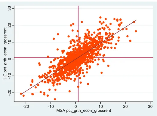
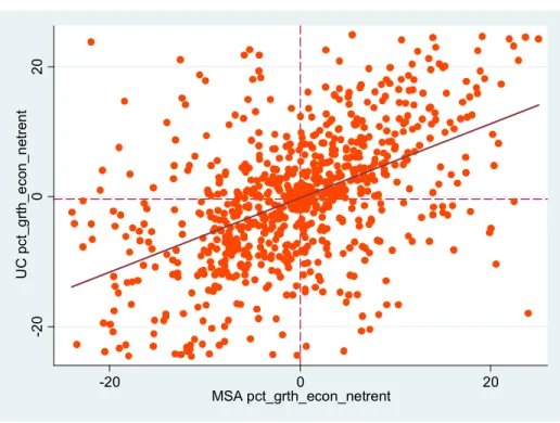
[Figure 21] Relation of the Growth Rate of Gross Rents between UC and MSA ... 45

[Figure 22] Relation of the Growth Rate of Net Rents between UC and MSA ... 46

[Figure 23] Changes in Economic Rental Rates (%) ... 49

[Figure 24] Average Rental Growth from 1993 to 2012... 50

[Figure 25] Relation of the Growth Rate of Economic Rents between UC and MSA ... 51

[Figure 26] Average Cap Rates of 50 Metropolitan Areas ... 55

[Figure 27] Average Cap Rates from 2003 to 2012 ... 56

[Figure 28] Relation of the Cap Rates between UC and MSA ... 57

[Figure 29] Changes in Cap Rates of 51 Metropolitan Areas (%) ... 60

[Figure 30] Average Cap Rates from 2003 to 2012 ... 60

[Figure 31] Relation of the Cap Rates between UC and MSA ... 61

[Figure 32] Relation between Population Growth Rates and Cap Rate Levels of UC ... 66

[Figure 33] Relation between Population Growth Rates and Cap Rate Levels of MSA ... 66

[Figure 34] Differences in Cap Rates and Population Growth Rates between UC and MSA ... 67

[Figure 35] Relation between Population Growth Rates and Cap Rate Levels of UC ... 68

[Figure 36] Relation between Population Growth Rates and Cap Rate Levels of MSA ... 68

[Figure 37] Differences in Cap Rate Levels and Population Growth Rates of UC and MSA ... 69

[Figure 38] Relation between Cap Rate Levels and Employment Growth Rates of UC ... 70

[Figure 39] Relation between Cap Rate Levels and Employment Growth Rates of MSA ... 70

[Figure 40] Differences in Cap Rate Levels and Employment Growth Rates between UC and MSA ... 71

(11)

M.I.T. | TABLE OF FIGURES 11

[Figure 42] Relation between Cap Rate Levels and Employment Growth Rates of MSA ... 72

[Figure 43] Differences in Cap Rate Levels and Employment Growth Rates between UC and MSA ... 73

[Figure 44] Scatter Diagram of Economic Gross Rents and Cap Rate Levels of UC ... 74

[Figure 45] Scatter Diagram of Economic Net Rents and Cap Rate Levels of UC ... 74

[Figure 46] Scatter Diagram of Economic Gross Rents and Cap Rate Levels of MSA... 75

[Figure 47] Scatter Diagram of Economic Net Rents and Cap Rate Levels of MSA ... 75

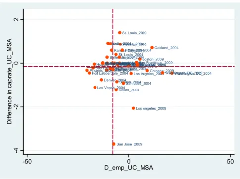
[Figure 48] Scatter Diagram of Differences in Cap Rates and Gross Rental Growth Rates between UC and MSA ... 76

[Figure 49] Scatter Diagram of Differences in Cap Rates and Net Rental Growth Rates between UC and MSA ... 77

[Figure 50] Difference in Gross Rental Growth Rates between UC and MSA (average from 2003 to 2012) ... 78

[Figure 51] Difference in Cap Rates between UC and MSA ... 78

[Figure 52] Difference in Net Rental Growth Rates between UC and MSA(average from 2003 to 2012) 78 [Figure 53] Difference in Cap Rates between UC and MSA ... 78

[Figure 54] Scatter Diagram of Economic Rents and Cap Rates of UC ... 83

[Figure 55] Scatter Diagram of Economic Rents and Cap Rates of UC ... 84

[Figure 56] Differences in Cap Rate Levels and Rental Rates beween UC and MSA ... 85

[Figure 57] Difference in Rental Growth Rates between UC ... 86

(12)

12 TABLE OF TABLES | M.I.T.

TABLE OF TABLES

[Table 1] Criteria for Zone Definition ... 22

[Table 2] Summary of Defined Zones ... 23

[Table 3] Land Area Changes ... 25

[Table 4] Summary of population changes ... 30

[Table 5] Summary of Employment Data ... 34

[Table 6] Summary of the Rental Rate Data ... 39

[Table 7] Summary of the Rental Rate and Vacancy Data ... 39

[Table 8] Summary of the Gross Rental Rate Data... 42

[Table 9] Panel Model of Economic Rents Growth Rates between UC and MSA ... 47

[Table 10] Panel Model of Economic Rental Growth Rates between UC and MSA ... 48

[Table 11] Summary of the Rental Rate Data ... 49

[Table 13] Summary of Transaction Data ... 53

[Table 14] Summary of the Cap Rate Data ... 53

[Table 15] Summary of Cap Rate Data by Zone ... 55

[Table 16] Panel Model of Cap Rates between UC and MSA ... 59

[Table 17] Summary of Average Cap Rates of 51 Metropolitan Areas ... 59

[Table 19] List of Regression Model Variables ... 79

[Table 20] Panel Model of Economic Gross Rents and Cap Rates of UC ... 80

[Table 21] Panel Model of Economic Gross Rents and Cap Rates of MSA ... 81

[Table 22] Panel Model of Economic Net Rents and Cap Rates of UC ... 82

[Table 23] Panel Model of Economic Net Rents and Cap Rates of MSA ... 82

[Table 24] Panel Model of Cap Rates and Economic Rent Growth Rates of UC ... 87

[Table 25] Panel Model of Cap Rates and Economic Rent Growth Rates of MSA... 88

[Table 26] List of Regression Model Variables ... 90

[Table 27] Regression Model of Determinants of Gross Rental Growth Rates ... 91

[Table 28] Regression Model of Determinants of Population Growth Rates ... 94

[Table 29] Regression Model of Determinants of Population Growth Rates with an Additional Variable 95 [Table 30] Regression Model of Determinants of Employment Growth Rates ... 96

(13)

M.I.T. | CHAPTER 1 INTRODUCTION 13

CHAPTER 1 INTRODUCTION

Until 2000’s, population and employment have been growing rapidly in suburban areas while most central cities have been declining or growing slowly. (Voith, 1992) That is, the population and employment centers of the United States have been undergoing a process of decentralization. (Garner, 2002) According to Garner (2002), most of the large metropolitan areas in the United States have had the

majority of employment and population in the suburbs rather than in the central cities.1_{However, we have}

recently observed significant changes in which corporate offices and residential buildings have been relocated from the suburbs back into the city and, in terms of rents and occupancy rate, the properties in the cites have been outperforming those in suburbs. Does the observation mean that there is a real economic movement back into the cities by firms or households? This study raises a question of whether the shift acts as a determinant of real estate performances.

1.1 Research Background and Motivation

Recently, there have been active debates on the “back to the city” movements. According to Wieckowski (2010), “the suburbs have lost their sheen; Both young workers and retiring Boomers are actively seeking to live in densely packed, mixed-use communities that don’t require cars- that is, cities or revitalized

outskirts in which residences, shops, schools, parks, and other amenities exist close together.” 2_In

addition, Wieckowski (2010) states that “companies such as United Air Lines and Quicken Loans are getting a jump on a major cultural and demographic shift away from suburban sprawl. The change is

imminent, and business that don’t understand and plan for it may suffer in the long run.” 3

Christie also mentioned, “The trend, which began in the late 1990s, marks a reversal of the post-war

urban flight to the suburbs. Now, it’s strengthening”. 4_{There is another recent discussion on “back to the}

movement”, written by Jaffe on the Atlantic Cities. “The silver lining for urban advocates was the city core. Even in places that experienced general declines in city population, such as St. Louise, downtowns

showed some impressive residential growth.” 5

Considering these arguments, however, this study questions whether these relocations of firms or households lead any real economic movement back into the cities. If there is any movement, how does this trend drive any changes in the commercial real estate properties? Does it significantly affect the

1_{Laurence Garner, Decentralization of Office Market and The Effects on Rates of Return, 2002} 2_{Ania Wieckowski, Back to the City, Harvard Business Review, 2010}

3_{Ania Wieckowski}

4_{Les Christie, Cities are hot again, CNNMoney.com, 2006} 5_{Eric Jaffe, So are people moving back to the city or not?, 2011}

(14)

14 CHAPTER 1 INTRODUCTION | M.I.T.

performance of properties in the cities as opposed to the other areas? Does the performance of properties in the city exert any influence on the investors who prefer commercial real estates in UC metropolitan areas?

1.2 Problem Statement and Research Objectives

As Jaffe stated, the finding of the “back to the city” movement also caused additional layer of the debate on the downtown-suburban migration. Cox and Kotkin argued, “Cities are even having trouble retaining younger population groups, calling them temporary way stations before people migrate somewhere

else-namely, the suburbs.” 6_{According to Jaffe, there was a disagreement with them, pointing out that “their}

analyses failed to properly define the terms city and suburb.” 7_{It is important to note that, without a clear}

identification of the specific regions the result would distort the actual movement and cause misunderstanding of the change.

Considering a number of research have been focused on real estate pricing across sections, the recent debate arouses the interest in investment return variations in accordance with geographic locations. That is, if the relocations of office and housing occur with a significant amount, the alteration would lead a reaction of real estate commercial markets, affecting performances such as rental income and price of properties. With this hypothesis, this study raises a question of whether this shift acts as a determinant of real estate performances. If so, does the pricing of commercial properties effectively respond to the market transformation? Are there any myths or misconceptions about the real estate pricing?

1.3 Research Scope, Assumptions, and Framework

Answering the questions requires several considerations, taking the issues in previous literatures into account. First, a defining “downtowns” is an inevitable element to assess population growth and employment shifts based on the specific area in a city relative to the rest of the city and to compare the growth and performance in two parts of a metropolitan area. Second, identifying the measurements of demographic movements and properties performance is an important factor in order to examine the difference between the two areas and as so to quantify the impact of the movement within the area. Third, collecting data in accordance with the measurements is an essential part so as to understand empirical market conditions and to produce compelling results. Lastly, devising a model is the critical component that explains observations and effects among the indicators.

6_{Eric Jaffe}

(15)

M.I.T. | CHAPTER 1 INTRODUCTION 15

Throughout this process, this thesis intends to provide the quantitative approach that examines impacts of economic movement between downtowns and suburbs on commercial real estate markets and to address the relation between the economic movement and properties pricing within a metropolitan market. In addition, it is hoped that this thesis will be utilized by investors and developers as a tool for assessing their potential sub-markets in the US metropolitan areas.

1.3.1 Scope and Assumptions

This study observes the trends and interactions between downtowns and suburbs over 23 years and across 69 Metropolitan Statistical Areas (MSAs) in the United States. It uses population, employment, rental income, and investment return as the four major indicators. The analysis is conducted on two property types: office and multifamily housing.

In order to measure the migration between a city center and the broader city, this study employs population and employment as parameters. The reason why this study examines the population and employment is because these data not only demonstrates the change in city size but also presents the demand side’s indication of office and apartment properties. Therefore, using the data allows this study to describe the relation between demographic changes and real estate markets. The data is obtained by the US Census Bureau.

The gauge used for economic performances is the economic rent, i.e., a property’s rent multiplied by its occupancy rate. The reason why this research uses economic rent as an indicator is because the economic

rent is the most reliable rental rates that reflect the conditions of a competitive and open market.8_Thus,

examining the data enable the research to capture the realistic economic performances of properties. The research explores the rental data from 1993 to 2012, which is provided by CBRE Econometric Advisors (CBRE EA, formerly Torto Wheaton Research), the leading real estate research firm owned by CBRE, the largest real estate service company.

The measurement used for investment performances is the capitalization rate (cap rate), which is “the

ratio of current net operating income to valuation”.9 _{The reason why this study employs the cap rate is}

because the return rates “play a central role in real estate investment, financing, and valuation decisions, and average market-wide capitalization rates are widely quoted and followed as a gauge of current real

estate investment market conditions”.10_{The research explores the capitalization data from 2003 to 2012,}

8_{It is referred to http://www.investorwords.com/1645/economic_rent.html#ixzz21k3pnDd0 and}

http://appraisersforum.com/showthread.php?t=156120.

9_{Petros Sivitanides et al.,The determinants of appraisal-based capitalization rates, 2001}

(16)

16 CHAPTER 1 INTRODUCTION | M.I.T.

which is originally provided by Real Capital Analytics (RCA), a global research and consulting firm focused on the investment market for commercial real estate, and processed by CBRE EA.

While using data from RCA for office and multifamily properties, this research designs regression models that explore the population, employment, economic rents, and capitalization rates. Based on the real transaction data, this thesis provides a convincing analysis, taking most of the factors previously described in the literature into account. More importantly, it should be noted that this study is the first to examine RCA’s investment return data at a specific zone level within a metropolitan area, even though these data from RCA have been widely used in other research.

1.3.2 Thesis Outline and Framework

The thesis is structured by five major analyses along with background knowledge as follows. The second chapter reviews the previous research on the “back to the city” movement and the real estate pricing. The third chapter outlines the data and methodology used for the entire thesis. The fourth chapter presents the empirical results on population and employment changes between the center of cities and their broader areas. The fifth and sixth chapters provide the results on economic rental changes and capitalization rate levels between the separate areas within a metropolitan market. The seventh chapter describes the relationships among the four major measurements, considering their dissimilar effects between the distinct zones in a city. The eighth chapter examines determinants that lead the difference in performances between the two defined locations. The conclusion summarizes the findings and contributions, and suggests ideas for further study. Figure 1 illustrates the thesis framework as below.

[Figure 1] Thesis Framework

To Define the Zones within a Metropolitan Area

To Explore the Demographic Changes To Examine the Economic Performances To Discuss the Investment Performances

To Analyze the Relation between Demographic and Economic Changes and Investment Performances

To Explain the Determinants of the Differences in Performances

(17)

M.I.T. | CHAPTER 2 LITERATURE REVIEW 17

CHAPTER 2 LITERATURE REVIEW

This study reviews previous literatures on two major topics such as the demographic movement within the metropolitan areas and the difference of investment performances associated with geographical markets. First, the thesis discusses the recent articles and empirical studies about the economic movement between downtowns and suburbs. Second, this research endeavors to investigate the performance of properties across MSAs, the pricing model, and the determinants for office and residential pricing in the US markets. Finally, it addresses key issues related to the “back to the city” movement and geographical variation in investment returns, while building the ground of this study.

2.1 “Back to the City” Movement

In Harvard Business Review, Wieckowski states, “The suburbs have lost their sheen: Both young workers and retiring Boomers are actively seeking to live in densely packed, mixed-use communities that don’t require cars-that is, cities or revitalized outskirts in which residences, shops, schools, parks, and other

amenities exist close together.”11_{Furthermore, he cites, “In the 1950s, suburbs were the future; the city}

was then seen as a dignity environment. But today it’s these urban neighborhoods that are exciting and

diverse and exploding with growth”12_{, commented by University of Michigan architecture and}

urban-planning professor Robert Fishman.

In this article, the writer addresses the causes and effects of the intra-regional movement, while exemplifying the relocations of office and housing. He argues that this movement caused by the issues in suburban areas such as health problems and transportation costs. Moreover, the article mentions the effect, saying “A shift to an urban model affects corporate strategy – especially for retail businesses currently thriving in strip malls on busy commuting arteries. Firms base many decisions on store locations

and the types of customers served, and a move to the city changes both.”13

This argument arouses the question of whether there is a real “back to the city” movement and motivates this thesis to examine the economic movement within a metropolitan area. Despite the motivation, the article doesn’t present any quantitative approach to the topic because the writer focuses on addressing the concept of broader recent changes in cities. In short, the literature lacks the assessment of the urban shift and its impact, while it contributes to attract interests into the current trends of the economic changes in cities.

11_Wieckowski

12_Wieckowski 13_Wieckowski

(18)

18 CHAPTER 2 LITERATURE REVIEW | M.I.T.

Contrary to Wieckowski, Aaron M. Renn illustrates the topic with numerical data. In 2011, he wrote the article of “back to the city?” while using the migration data provided by the International Revenue Service. In the writing, he stresses, “There is intriguing evidence of a shift in intra-regional population dynamics in the migration numbers. The one bright spot was downtowns, which showed strong gains, albeit from a low base. Migration from the suburban counties to the core stayed flat or actually increased,

even late in the decade when again overall migration declined nationally.”14

This literature clearly discusses the back to the city movement with empirical data. It displays the changes of in and out migration with a specific scale such as “Migration Index” and “Migration Values”. In addition, the article provides the trend in four major cities in US over decade, saying “There has clearly been a shift affecting the net migration in these cities. In particular, the fact the in-migration from the

suburbs to the core held steady or even increased is a sign of some urban health.”15

However, he shows the limited approach to the clarification in the intra-regional migration. That is, the urban core’s definition used in the article is the combination of city and county. This issue was caused because the article used the data from the Internal Revenue Service, which aims to “track movements of

people around the country on a county-to-county and state-to-state basis”16. Therefore, the data and

definition are hardly applied to most of the US metropolitan areas since many places where have central cities also include their broader suburban areas. (Renn, 2011) Consequently, he only examined a limited number of cities that matches the data mapping: New York, Philadelphia, San Francisco, and Washington DC. In addition, he didn’t consider any other demographic data, except for IRS migration number, on economic movements in cities, so that the examination couldn’t describe the overall demographic changes in urban centers and broader cities, and failed to explore market-specific characteristics.

None of these articles clearly identified the definition of city centers and suburbs mentioned in the findings. There is also the limit of quantitative approaches to the economic movement in cities. Because of these constraints, the articles examined a limited number of city or specific cases rather than an extensive range of markets. Furthermore, few studies have focused on the relationship between the “back to the city” movement and the real estate markets.

14_{Aaron M. Renn, back to the city?, Newgeography.com, 2011} 15_Renn

(19)

M.I.T. | CHAPTER 2 LITERATURE REVIEW 19

2.2 Differences in Investment Returns across Geographical Locations

Petros Sivitanides et al. (2001) say, “Capitalization rate levels exhibit persistent differences across markets as a result of variations in fixed market characteristics that influence investor perceptions of risk and/or income growth expectations. Movements in market-specific capitalization rates strongly incorporate components that are shaped by the behavior of the local market and, more specifically, by the

time path of rental growth and rent levels relative to their historical averages.”17

According to Sivitanides (2001), his paper was the first study to explore capitalization rates at the local level, based on the property database obtained from National Council of Real Estate Investment Fiduciaries (NCREIF). Besides, the paper shows different approach from others because it “used a

panel-based model, rather than just time series.”18_{Applying both time series and cross-section to the model}

enables the analysis to enrich and to obtain thorough statistical results. (Sivitanides et al., 2001)

Despite these accomplishments, the paper has a few limits such as using the NCREIF data and analyzing the capitalization rate at MSA level; the writer used periodic appraisals data from NCREIF rather than actual transaction data of property values; the paper analyzed the variation in capitalization rate levels of MSAs, leaving further study on “the issues of variation of capitalization rates across sub-markets within

the same metropolitan area, or alternatively, between suburban versus downtown locations.”19_{In addition,}

the paper restricted the number of market to 14 metropolitan areas in the US.

Doina Chichernea et al. (2007) studied cross sectional differences in cap rates across the US metropolitan markets. In the study, they say, “while capitalization rates have received a lot of attention in recent empirical real estate literature, most research has focused on explaining the patterns in cap rates over time or the variation in cap rates across different property types. Our study extends the existing literature by addressing a question that has received far less attention than needed, namely what are the factors driving

the geographical cross-sectional variation in these cap rates.”20

In the paper, the writers focus on the determinants that cause the spatial variation in capitalization rates across the geographical markets and explore models with variables such as demand, supply, liquidity, risk, and their interaction. (Chichernea et al., 2007) The result shows that “such variations are largely

determined by the supply constraints and the liquidity of different geographical markets.”21_Meanwhile,

they found that there is no strong effect of demand growth on capitalization rates. (Chichernea et al.,

17_{Petros Sivitanides et al., The determinants of appraisal based capitalization rates, 2001} 18_{Sivitanides et al.}

19_{Sivitanides et al.}

20_{Doina Chichernea et al., A cross sectional analysis of cap rates by MSA, 2007} 21_{Chichernea et al.}

(20)

20 CHAPTER 2 LITERATURE REVIEW | M.I.T.

2007) Finally, it addresses the contribution of the study, saying “uncovering the driving factors behind geographic variation of cap rates is important as it can help us better understand and identify conditions of

disequilibrium among different markets.”22

Even though the paper provides the understanding in major factors driving the geographical variation in capitalization rates, it remains several limits in the approach. First, the study examined 22 MSAs, a limited number of metropolitan areas, which might be hard to explain an extensive range of markets. Second, this article limits the scope of analysis on multifamily properties from 2000 to 2005, which would cause the model a difficulty in taking the time effects into account. In addition, since the writer focused on the spatial variation in capitalization rate at the MSA level, he didn’t explore differences in investment returns across specific areas within the same metropolitan market.

As Sivitanides et al. (2001) said in their paper, “Real estate capitalization rates have been the focus of a growing body of empirical research. A few other studies have attempted to explore spatial differences in capitalization rates, across either broadly defined regions or markets within a given metropolitan area (Sirmans et al., 1986; Saderion et al., 1994; Grissom et al., 1987; Hartzell et al., 1987; Sivitanides et al.,

2001)”23 Especially in order to explain the impact of the “back to the city” movement on real estate

markets, it is essential to analyze how the capitalization rate level varies between downtowns and suburbs.

22_{Chichernea et al.}

(21)

M.I.T. | CHAPTER 3 DATA AND METHODOLOGY 21

CHAPTER 3 DATA AND METHODOLOGY

This chapter gives the description of data and methodology. First, it introduces the re-definition of

“downtowns”24_{, which was identified by CBRE EA. Second, this chapter clarifies four major}

measurements used for assessing the economic movement within a metropolitan area. Third, the section describes the data and the sources. Lastly, this part presents the methodology used in the study.

3.1 Zone Definition: Urban Core, Center City, and MSA

3.1.1 Definition Methodology

In order to examine the difference between city cores and broader cities, it is critical to ascertain the specific areas with reasonable criteria. This thesis uses the new definition of downtowns identified by CBRE EA; the research firm re-defines a downtown as the area where is broader than Central Business

District (CBD)25 and narrower than central city. (CBRE EA, 2012) According to CBRE EA, central cities

defined by jurisdictional extent are hard to use as central locations because the areas are so far-reaching that they cover other areas where have particularly suburban characteristics. (CBRE EA, 2012) Moreover, the firm pointed out that “CBD or downtown definitions are too narrow, focusing mainly on just business districts, and so will be unable to adequately capture variations in demographic and employment trends

with acre taking place in cities.”26_{Considering these issues, this thesis uses the newly defined}

downtowns, which are called the city’s Central Urban Core or Urban Core (CUC or UC).

The firm re-defined downtowns with several characteristics: first, the major employment spots such as financial and business districts within each city; second, major attractions such as shopping center, museums, theaters and sports complexes; third, main residential areas where are densely packed and walkable places of living, enabling residents to work at the employment spot and walk to the commercial and cultural areas. (CBRE EA, 2012)

The methodology that CBRE EA used for re-defining urban core is as below.

24_{This study uses the market definition used by CBRE EA. The firm defined downtown as “the sum of all}

submarkets associated with the primary office business activity area of a city. Market areas with an approved “downtown” designation in most cases will have a significant number of high-rise office buildings that represent the majority of the square footage of these submarkets.”

25_{CBRE EA defines this area, saying “The Central Business District (CBD) is generally a submarket and is given}

this name. The Central Business District generally will not represent all of the properties within the “Downtown” area of a particular city.”

(22)

22 CHAPTER 3 DATA AND METHODOLOGY | M.I.T.

“To re-define this kind of “Central Urban Core” we developed a Google Earth GIS-based application that overlaid a variety of data. We began with the existing boundaries currently used by the leasing agents of CBRE for identifying “downtown” office buildings. We then superimposed on them current ZIP code boundaries. The primary reason for using zip codes as building blocks for our new definitions is that ZIP is the smallest level of geography at which employment and demographic data is readily available. Such an approach also allowed us to develop a set of definitions that are not tied to any one data vendor but instead to publicly available sources such as Decennial Census and ZIP Code Business Patterns data.”

[Figure 2] Zone Definition

In order to re-define zones within MSA, CBRE EA used criteria: 1) population density and growth, 2) income levels, and 3) inclusion of special uses. The detailed requirements are as Table 1.

[Table 1] Criteria for Zone Definition27

Items Criteria Requirements

Population Density _Growth

Greater than average population density Positive growth

Between 2000 and 2010 Income Per capita income levels At least metropolitan average of income

Uses Special uses Universities, museums, convention centers, _{sports complexes, etc}

3.1.2 Defined Zones

Based on the methodology of defining zones, CBRE EA examined 69 metropolitan areas and identified Urban Cores for each city. For office markets, 69 metropolitan areas have been classified while 51 urban

27_{CBRE EA}

MSA Center City Urban Core MSA Center City Urban Core

(23)

cores defined. For multifamily housing, of 46 MSAs, 46 Urban Cores have been identified. The newly defined cores vary in the size and the number of ZIP codes ranging from a single code to around 30

ones.28

[Table 2] Summary of Defined Zones

Markets Central Urban Core (UC) Center City (CC) MSA

Office 51 49 69

MFH 46 41 46

Of the defined zones, this research focuses on the Urban Cores and MSAs, leaving the Center City in the further study. This is because the comparison between Urban Core and MSA allows the study to clearly explain the back to the city movement and its effect on real estate markets. In addition, examining two areas helps extensive cross-section analysis since Core markets have been identified more than Center City. The example of the defined zones is as Figure 2, which shows the case of the Boston metropolitan area. The green area is MSA, the blue part is Center City, and the red is Urban Core.

[Figure 3] Defined Zones in Boston

28_{CBRE EA}

(24)

3.2 Data Description

This thesis employs the four types of data to answer the research question on the geographical variation. The four major indicators used are population, employment, rental incomes, and investment returns. In addition, the study focuses on two property types: office and multifamily housing.

This study observes the trends and interactions between downtowns and suburbs over 23 years and across 69 Metropolitan Statistical Areas (MSAs) in the United States. This thesis uses population, employment, rental income, and investment return as the four major indicators. The analysis is conducted on two property types: office and multifamily housing.

In order to measure the migration between a city center and the broader city, this study employs population and employment as parameters. The reason why this study examines the population and employment is because these data not only demonstrates the change in city size but also presents the demand side’s indication of office and apartment properties. The data is obtained by the US Census Bureau.

3.2.1 Population Data

In order to measure the migration between an urban core and MSA, this study examines population as a parameter. The reason why this study explores the population is because this data not only demonstrates the change in city size but also acts as the demand indication of multifamily housing market. Using

demographic data at the local market level allows this study to resolve the issue29_{in which previous}

article had. The data consists of the population level of 52 MSAs over last three decades from 1990 to 2010, the data originally obtained by the US Census Bureau and processed at the newly defined zone level by CBRE EA. Since population data is provided every decade, this study examines the demographic changes in every 10 years.

3.2.2 Employment Data

In order to examine the effect of the job market within a metropolitan, this study also uses employment data. The reason why this study scrutinizes the employment is because this data demonstrates the city characteristic of its size and growth as well as indicates the demand side of the office property market. The data comprises of the employment level of 52 metropolitan markets from 1994, 1999, 2004, and 2009 at ZIP code level, originally provided by the US Census Bureau and handled at the specific zone level by

29_{Renn(2011) didn’t consider any demographic data on economic movements in cities except for the IRS migration}

number, so that the study couldn’t describe the overall demographic changes in urban centers and broader cities, and failed to explore market-specific characteristics. For the detail, please refer to Chapter 2 Literature Review.

(25)

CBRE EA. Since the employment data at the zip code level is not provided until 1994 and also is not currently available for 2010, this study detects the changes of job markets in last 15 years.

Through the data transition from a ZIP level to a zone level, CBRE EA found that there were land area changes at the MSA level between 2000 and 2010. Of 52 MSAs used in the study, some metro areas had gone through fairly large changes which vary among the newly defined zones. Despite the finding, the study lets the boundary changes have their impact. Table 3 below shows the metropolitan areas where the land area changed more than 5%.

[Table 3] Land Area Changes

3.3.3 Property Data

The study uses property rental data as the gauge for economic performances of offices and apartments. Rather than using the rental rate level, this study examines the economic rent, i.e. a property’s rent multiplied by its occupancy rate. The reason why this research uses economic rent as an indicator is because the economic rent is the most reliable rental rates that reflect the conditions of a competitive and

open market.30_{The data on rental rates from 1993 to 2012 comes from CBRE EA, which are thousands of}

actual lease transactions in each market. The rental rates consist of 3,772 of asking gross rates and 3,349 of asking net rates for offices in 69 MSAs, and 2514 of rental data for multi-housing in 46 MSAs originating from databases compiled by the CBRE EA. Jennen et al. offers the reason why asking rents was used in office rental analysis, citing Dunse and Jones (1998). They reasoned, saying “The first explanation is the proprietary nature of office transaction rents, which makes analysis based on

30_{It is referred to http://www.investorwords.com/1645/economic_rent.html#ixzz21k3pnDd0 and}

(26)

transaction rents often impossible. The second, more sensible, rationale mentioned is the existence of

unknown incentives in quoted transaction rents, which distort the analysis of rent levels.”31

3.3.4 Transaction Data

In order to capture investment performances, this study uses the capitalization rate, which is “the ratio of

current net operating income to valuation”.32_{The reason why this study employs the cap rate is because}

the return rates “play a central role in real estate investment, financing, and valuation decisions, and average market-wide capitalization rates are widely quoted and followed as a gauge of current real estate

investment market conditions”.33_{The research explores the capitalization data from 2003 to 2012, which}

is originally provided by Real Capital Analytics (RCA), a global research and consulting firm focused on the investment market for commercial real estate, and processed by CBRE EA. Originally, the RCA reports monthly series of average transaction cap rates, dating back to 2001. However, this study uses the data from 2003 to 2012 because the data from 2001 to 2002 are quite incomplete that it is hard to apply to the examination based on the Urban Cores and MSAs which are defined at ZIP code level. Using the transaction data enables the study to conduct a compelling analysis, providing actual movements in cap rates over time. Moreover, compared to NCREIF, “RCA data is derived from a broader sample of

properties including institutional transactions”.34

3.3 Panel Data Regression Model

Using data described above, the author applies the panel regression model to examine the effect of economic movements on properties performances. Since this research employs major indicators such as the population, employment, economic rents, and capitalization rates over 20 years and across 69 metropolitan areas, this study utilizes a panel-based model rather than just time series or cross section. Before illustrating the model used, this section briefly reviews the panel data and the regression model.

3.3.1 What is Panel Data?

Unlike time series or cross-section data, panel data allows to be investigated the same cross-sectional data over time. For this reason, the panel data is also called other names such as pooled data or combination of time series and corss-section data. The data basically enables researchers to obtain robust results, by letting them analyze the observations over time in cross sections. The advantages of panel data are clearly mentioned in the book of Basic Econometrics as follows:

31_{Maarten G.J. Jennen et al., The Effect of Clustering on Office Rents: Evidence from the Amsterdam Market, 2009} 32_{Petros Sivitanides et al.}

33_{Jim Clayton et al.} 34_{Jim Clayton et al.}

(27)

“By combining time series of cross-section observations, panel data give more informative data, more variability, less collinearity among variables, more degrees of freedom and more efficiency; By studying the repeated cross section if observations, panel data are better suited to study the dynamics of change; Panel data can better detect and measure effects that simply cannot be observed in pure cross-section or pure time series data; In short, panel data can enrich analysis in ways that may not be possible if we use

only cross-section or time series data.” 35

3.3.2 Why Use the Panel Data Regression Model?

The research uses panel data regression model in order to explore the relation between Urban Cores and MSAs based on several data sets such as population, employment, rents, and capitalization rates over 20 years and across 69 metropolitan markets. The basic formula of panel data regression model is as below.

( ) = + ( )+ ( )+ ( ) (1)

where j stands for the jth metropolitan market and t for the tth time period. The equation shows the effect of X(jt) on Y(jt), indicating that a unit of increase in X(jt) leads to gain the amount of change in Y(jt). The dummy variable of FE(j) captures the metropolitan fixed effects; the statistically significant coefficient of the dummy indicates that there are market-specific characteristics that explain the difference between markets. Likewise, another dummy variable of FE(t) measures the time fixed effects; if the coefficient of the dummy is statistically significant, the specific time gives impact on the dependent variable. Since regression model allows the researchers to analyze the impact of an explanatory variable to the independent variable, this study use the model for measuring the relation between two designated areas within MSA. Since this research uses a different number of observations among metropolitan areas, the data is an unbalanced panel and the regression model analyzes the effects of variables based on the unbalanced data set.

3.3.3 Panel Data Regression Model with the Fixed Effects

The models developed in this research assume that there are both individual metropolitan effect and time effect together, which means that the intercept varies over cross-section as well as time. Therefore, the regression model includes the metropolitan dummies as well as time dummies. This study allows the fixed effects in the model because adding dummies helps the data set enrich and results in a compelling outcome. Sivitanides (2001) also clarified the reason why dummies are used in the model, stating “Since fixed effects are normally part of a panel analysis, including them was almost a requirement; Once included in the analysis, adding any other variables that exhibited only cross-section variation would be

(28)

redundant; Thus, the fixed effects will be interpreted largely as reflecting market-specific differences and

time-specific variations”.36

3.3.4 Scatter Diagram and Linear Regression

While this thesis uses the panel data regression model, it also explores the observation using scatter diagrams with simple linear regressions. Since this study examines the correlation and differentials between two areas within a metropolitan market, the scatter diagram plotting the distribution of data

allows the analysts to simply find out corresponding of a parameter to a given or fixed value.37_{That is,}

“Scatterplots can show you visually the strength of the relationship between the variables, the direction of

the relationship between the variables, and whether outliers exist.”38

36_{Petros Sivitanides et al.}

37_{web2.concordia.ca/Quality/tools/25scatter.pdf; personnel.ky.gov/NR/rdonlyres/CF0C40D5.../ScatterDiagrams.pdf} 38_{http://www.r-statistics.com/2010/04/correlation-scatter-plot-matrix-for-ordered-categorical-data/}

(29)

M.I.T. | CHAPTER 4 POPULATION & EMPLOYMENT CHANGES 29

CHAPTER 4 POPULATION & EMPLOYMENT CHANGES

Answering the question as to the “back to the city” movement requires investigating the changes in population and employment within the metropolitan area. As previous literatures pointed out, the only part that shows a strong gain in population was downtown within a city. (Renn, 2011) To examine the difference between downtowns and suburbs, the definition of UC and MSA is employed. The goal of this chapter is to measure any shift in intra-regional population and employment and to discuss the trends across the metropolitan markets over decades.

4.1 Data and Methodology

In order to measure the migration between an urban core and MSA, this study examines population as a parameter. Using demographic data at the local market level allows this study to compare the performance of the city core as opposed to MSA. In addition, measuring the level of population provides the market-specific characteristics such as the size and the growth rate of a market as well as the level of demand in real estate markets. The population data draws from 52 MSAs from 1990 to 2010. Since the census data is provided every decade, this study examines the trend in population changes in every 10 years, focusing on comparison between the two specific markets.

The level of employment is also an important indicator of demographic dynamics. Therefore, this study tracks employment data so as to examine the changes in the job market within a metropolitan area. Scrutinizing the employment also offers the regional characteristics of the market size and the growth rate. The level of employment also indicates the demand side of the office property market. The data comprises of the employment level of 52 metropolitan markets from 1994, 1999, 2004, and 2009 at ZIP code level, originally provided by the US Census Bureau and handled at the specific zone level by CBRE EA. Since the employment data at the zip code level is not provided until 1994 and also is not currently available for 2010, this study detects the changes of job markets in last 15 years.

4.2 Population Changes between Urban Core and MSA

Based on the newly defined zones, this section compares the demographic changes between Urban Cores and MSAs. By examining the trends by year, metropolitan areas, and cross-specific sections, the migration between cores and suburbs is illustrated from 1990 to 2010.

(30)

30 CHAPTER 4 POPULATION & EMPLOYMENT CHANGES | M.I.T. 4.2.1 Population Changes by Year

Last two decades, the trend in population dynamics clearly shows the new aspect of awakening of the US city, at least in terms of the population growth rate. The average of UC population from 1990 to 2000 decreases by around 4,580 per city while the average population in MSA increases by about 322,452 per city during the same period. This number testifies that there was the decentralization during the 1990s. However, when it comes to the 2000s, the city and suburban growth moderates the view of suburbanization phenomenon. As seen in Table 4, the intra-regional movement to UC increased by 4,827 per city while the gain of MSA was 289,611 of population over the decade, indicating that the demographic growth rate of UC has been greater than that of MSA over 10 years. This result renders that the urban area has been growing rapidly, turning the net changes in population from the loss to the gain since 2000. In respect of the growth rate, there was only one UC that grew faster than MSA in 2000 but, in 2010, the number of UC that shows greater growth rate in population increased by 11, which takes 21.15% of the total. Figure 4 and 5 show the result of the change in population between downtowns and suburbs.

[Table 4] Summary of population changes

1991~2000 2001~2010

Total Average of Population Growth in UC -4,580 4,827 Total Average of Population Growth Rate in UC -3.48% 3.80% Total Average of Population Growth in MSA 322,452 289,611 Total Average of Population Growth Rate in MSA 14.66% 11.48%

[Figure 4] Population Growth Rates

between UC and MSA [Figure 5] Comparison of Growth Rates between UC and MSA39

39_{The number indicates that the number of zones where show the better performance between UC and MSA. That}

is, in 2000, the only one UC grew faster than the MSA. In 2010, however, 11 UC outperformed MSA in terms of the population growth. -8% -4% 0% 4% 8% 12% 16% 2000 2010

Total Average of pct_grth_popUC Total Average of pct_grth_popCC Total Average of pct_grth_popMSA

0% 20% 40% 60% 80% 100% 2000 2010 1 11 51 41 UC MSA

(31)

M.I.T. | CHAPTER 4 POPULATION & EMPLOYMENT CHANGES 31 4.2.2 Population Changes by Zone

First of all, this section describes the demographic changes in MSA. Figure 6 provides the difference in the growth rate across the US markets over two decades. The total average growth rate of these cities decreased from 14.66% to 11.48% and the population changes are +322,452 in 2000 and +289,611 in 2010. Of 52 MSAs, 29 cities grew slower in 2000s than 1990s, more than half of the cities.

Second, since 1990 the total average growth rate of population in UC increased from -3.48% to 3.80%, supporting an assertion of the urban renaissance. In the 1990s, UCs experienced, on average, the loss of 4,580 people per city. However, the same area gained the amount of 4,827 people per MSA in 2010, showing the dramatic change. As can be seen from Figure 6, the average growth rate of population in 2010 outperforms that in 2000. Of 52 MSAs, 44 UCs presented the rapider growth of population in 2000s than 1990s, the portion of 84.62%.

[Figure 6] Average of the MSA Population Growth Rate in 52 Metropolitan Areas from 1990 to 2010

-20 0 20 40 60 80 100 Al ba ny Al bu qu erqu e At la nt a Au st in Ba lti m or e Bo st on Ch ar lo tt e Ch ic ag o Ci nc in na ti Cl ev el an d Co lu m bu s Da lla s De nv er De tr oi t Fo rt L au de rd al e Fo rt W or th Ha rt fo rd Ho no lu lu Ho us to n In di an apo lis Jac ks on vi lle Ka ns as C ity La s Ve ga s Lo s An ge le s Lo ui sv ill e Me m ph is Mi am i Mi lw au ke e Mi nn ea po lis Na sh vi lle Ne w Y ork Oa kl an d Ok la ho m a Ci ty Or la nd o P hi la de lph ia Ph oe ni x Pi tt sb ur gh Po rt la nd Ra le ig h Sa cr am en to Sa lt La ke C ity Sa n An to ni o Sa n D ie go Sa n Fr an ci sco Sa n Jo se Se at tle St . L ou is Ta m pa To le do Tu cs on Wa sh in gt on , D C Wi lm in gt on

(32)

32 CHAPTER 4 POPULATION & EMPLOYMENT CHANGES | M.I.T.

[Figure 7] Average of the UC Population Growth Rate in 52 Metropolitan Areas from 1990 to 2010

4.2.3 Population Changes between UC and MSA

As clearly rendered in Figure 8 and Figure 9, the different facet of the movement between 1990 and 2010 is observed regarding the population growth rate between UC and MSA. In the chart of the year of

200040_{, San Francisco is the only city that the UC growth rate is greater than MSA growth rate. Moreover,}

the urban cores in the most of metropolitan areas underwent negative growth rates, 40 UCs of 52 in total. On the other hand, most of MSA grew faster from 1991 to 2000, noting that there are only three places that the number of people in the area decreased.

However, this trend of suburbanization changed from 2001 to 2010. During the period, the fewer number of UC are notified that their population decreased, indicating that the total average growth rate is 3.80% in 2010. In contrast, MSAs show slower growth in population, decreasing the grow rate from 14.66% to 11.48%. Even though the total average growth rate of MSA is greater than that of UC, it is important to note that there are changes in the urban growth in US 52 metropolitan areas since 2000.

40_{The average of the population growth rate in 2000 indicates the change from 1991 to 2000. Likewise, the 2010}

growth rate of population calculated from the difference from 2001 to 2010. -60 -40 -20 0 20 40 60 80 100 120 Al ba ny Al bu qu erqu e At la nt a Au st in Ba lti m or e Bo st on Ch ar lo tt e Ch ic ag o Ci nc in na ti Cl ev el an d Co lu m bu s Da lla s De nv er De tr oi t Fo rt L au de rd al e Fo rt W or th Ha rt fo rd Ho no lu lu Ho us to n In di an apo lis Jac ks on vi lle Ka ns as C ity La s Ve ga s Lo s An ge le s Lo ui sv ill e Me m ph is Mi am i Mi lw au ke e Mi nn ea po lis Na sh vi lle Ne w Y ork Oa kl an d Ok la ho m a Ci ty Or la nd o P hi la de lph ia Ph oe ni x Pi tt sb ur gh Po rt la nd Ra le ig h Sa cr am en to Sa lt La ke C ity Sa n An to ni o Sa n D ie go Sa n Fr an ci sco Sa n Jo se Se at tle St . L ou is Ta m pa To le do Tu cs on Wa sh in gt on , D C Wi lm in gt on

(33)

M.I.T. | CHAPTER 4 POPULATION & EMPLOYMENT CHANGES 33

[Figure 8] Average of the Population Growth Rate between UC and MSA in 2000

[Figure 9] Average of the Population Growth Rate between UC and MSA in 201041

41_{There are a couple of dramatic increase in UC such as Cincinnati and Hartford. These changes might be explained}

by the changes of land area and, accordingly, increase in the number of ZIP codes which are the criteria for aggregation of the Census data.

-60 -40 -20 0 20 40 60 80 100 Al ba ny Al bu qu erqu e At la nt a Au st in Ba lti m or e Bo st on Ch ar lo tt e Ch ic ag o Ci nc in na ti Cl ev el an d Co lu m bu s Da lla s De nv er De tr oi t Fo rt L au de rd al e Fo rt W or th Ha rt fo rd Ho no lu lu Ho us to n In di an apo lis Jac ks on vi lle Ka ns as C ity La s Ve ga s Lo s An ge le s Lo ui sv ill e Me m ph is Mi am i Mi lw au ke e Mi nn ea po lis Na sh vi lle Ne w Y ork Oa kl an d Ok la ho m a Ci ty Or la nd o P hi la de lph ia Ph oe ni x Pi tt sb ur gh Po rt la nd Ra le ig h Sa cr am en to Sa lt La ke C ity Sa n An to ni o Sa n D ie go Sa n Fr an ci sco Sa n Jo se Se at tle St . L ou is Ta m pa To le do Tu cs on Wa sh in gt on , D C Wi lm in gt on

Average of grth_popMSA_2000 Average of grth_popUC_2000

-40 -20 0 20 40 60 80 100 120 Al ba ny Al bu qu erqu e At la nt a Au st in Ba lti m or e Bo st on Ch ar lo tt e Ch ic ag o Ci nc in na ti Cl ev el an d Co lu m bu s Da lla s De nv er De tr oi t Fo rt L au de rd al e Fo rt W or th Ha rt fo rd Ho no lu lu Ho us to n In di an apo lis Jac ks on vi lle Ka ns as C ity La s Ve ga s Lo s An ge le s Lo ui sv ill e Me m ph is Mi am i Mi lw au ke e Mi nn ea po lis Na sh vi lle Ne w Y ork Oa kl an d Ok la ho m a Ci ty Or la nd o P hi la de lph ia Ph oe ni x Pi tt sb ur gh Po rt la nd Ra le ig h Sa cr am en to Sa lt La ke C ity Sa n An to ni o Sa n D ie go Sa n Fr an ci sco Sa n Jo se Se at tle St . L ou is Ta m pa To le do Tu cs on Wa sh in gt on , D C Wi lm in gt on

(34)

34 CHAPTER 4 POPULATION & EMPLOYMENT CHANGES | M.I.T.

4.3 Employment Changes between Urban Core and MSA

Like the analysis on the population growth, the comparison in employment changes between UC and MSA is conducted based on the raw data obtained from US Census Bureau. Following the specifically defined zones, this study performs the analysis on the employment changes between Urban Cores and MSAs, illustrating the trend by year, metropolitan areas, and two identified zones using the data from 1994 to 2009.

4.3.1 Employment Changes by Year42

As not only shown by Table 5 but also expected, it is apparent that the employment growth has been slow down since 1994. The total average of growth rate in MSA is getting lower and lower, so that the MSA rate from 2005 to 2009 became -0.43%, decreasing average 4,745 employees per city. Unlike MSA, UC shows a recovery in the growth rate from -1.22% in 2004 to 1.85% in 2009.

The average of UC employment from 2000 to 2004 decreases by around 2,064 per city while the average

population in MSA increases by about 47,966 per city during the same period43_{. However, since 2005, the}

trend in the job growth of the city and suburban has been changed. As seen by Table 5, the job in UC increased by 3,088 positions per city while workers in MSA lost around 4,745 numbers of jobs for 5 years, indicating that the employment growth rate of UC has been improving during the period. This result describes that the MSA area has been left behind in rebound of job markets while UCs have been started creating jobs since 2004. In respect of the growth rate, there was only five UC that grew faster than MSA in 1999 but, in 2009, the number of UC that shows greater growth rate in employment increased by 21, which takes 40.38% of the total. Figure 10 and 11 show the result of the change in employment between urban centers and broader cities.

[Table 5] Summary of Employment Data

1994~1999 2000~2004 2005~2009 Total Average of Employment Growth in UC 8,242 (2,064) 3,088 Total Average of Employment Growth Rate in UC 5.12% -1.22% 1.85% Total Average of Employment Growth in MSA 158,848 47,966 (4,745) Total Average of Employment Growth Rate in MSA 17.51% 4.50% -0.43%

42_{The average of the employment growth rate in 1999 indicates the change of employment from 1994 to 1999. In}

the same way, the 2004 and 2009 growth rate of employment calculated by the difference from 2000 to 2004 and from 2005 to 2009 respectively.