Backward-forward search for manipulation planning
The MIT Faculty has made this article openly available.
Please share
how this access benefits you. Your story matters.
Citation
Garrett, Caelan Reed et al. “Backward-Forward Search for
Manipulation Planning.” 2015 IEEE/RSJ International Conference
on Intelligent Robots and Systems (IROS), September 28 - October
2 2015, Hamburg, Germany, Institute of Electrical and Electronics
Engineers (IEEE), December 2015: 6366-6373 © Institute of
Electrical and Electronics Engineers (IEEE)
As Published
http://dx.doi.org/10.1109/IROS.2015.7354287
Publisher
Institute of Electrical and Electronics Engineers (IEEE)
Version
Author's final manuscript
Citable link
http://hdl.handle.net/1721.1/111683
Terms of Use
Creative Commons Attribution-Noncommercial-Share Alike
Backward-Forward Search for Manipulation Planning
Caelan Reed Garrett, Tom´as Lozano-P´erez, and Leslie Pack Kaelbling
Abstract— In this paper we address planning problems in high-dimensional hybrid configuration spaces, with a particular focus on manipulation planning problems involving many ob-jects. We present the hybrid backward-forward (HBF) planning algorithm that uses a backward identification of constraints to direct the sampling of the infinite action space in a forward search from the initial state towards a goal configuration. The resulting planner is probabilistically complete and can effectively construct long manipulation plans requiring both prehensile and nonprehensile actions in cluttered environments.
I. INTRODUCTION
Many of the most important problems for robots require planning in high-dimensional hybrid spaces that include both the state of the robot and of other objects and aspects of its environment. Such spaces are hybrid in that they involve a combination of continuous dimensions (such as the pose of an object, the configuration of a robot, or the temperature of an oven) and discrete dimensions (such as which object(s) a robot is holding, or whether a door has been locked).
Hybrid planning problems have been formalized and ad-dressed in the robotics literature as multi-modal planning problems and several important solution algorithms have been proposed [1], [2], [3], [4], [5], [6], [7]. A critical problem with these algorithms is that they have relatively weak guidance from the goal: as the dimensionality of the domain increases, it becomes increasingly difficult for a forward-search strategy to sample effectively from the infinite space of possible actions.
In this paper, we propose the hybrid backward-forward (HBF) algorithm. Most fundamentally, HBF is a forward search in state space, starting at the initial state of the complete domain, repeatedly selecting a state that has been visited and an action that is applicable in that state, and computing the resulting state, until a state satisfying a set of goal constraints is reached. However, a significant difficulty is that the branching factor is infinite—there are generally infinitely many applicable actions in any given state. Furthermore, random sampling of these actions will generally not suffice: actions may need to be selected from very small or even lower-dimensional subspaces of the space of applicable actions, making it a measure 0 event to hit
Computer Science and Artificial Intelligence Laboratory, Massachusetts Institute of Technology, Cambridge, MA 02139 USA
[email protected], [email protected], [email protected]
This work was supported in part by the NSF (grant 1420927). Any opinions, findings, and conclusions or recommendations expressed in this material are those of the author(s) and do not necessarily reflect the views of the National Science Foundation. We also gratefully acknowledge support from the ONR (grant N00014-14-1-0486 ), from the AFOSR (grant FA23861014135), and from the ARO (grant W911NF1410433).
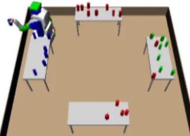
Fig. 1: A near-final state of a long-horizon problem.
an appropriate one at random. For example, consider the problem of moving the robot base to some configuration that may be the initial step of a plan to pick up and move an object. That configuration has to be selected from the small subset of base poses that have an inverse-kinematics solution that allows it to pick up the object. Or, in trying to select the grasp for an object, it may be critical to select one in a smaller subspace that will allow the object to be subsequently used for a task or placed in a particular pose.
HBF solves the exact planning problem by strongly focus-ing the samplfocus-ing of actions toward the goal. It uses backward search in a simplified problem space to generate sets of actions that are useful: these useful actions are components of successful plans in the simplified domain and might plausibly be contained in a plan to reach the goal in the actual do-main. The backward search constructs a reachability graph, working backward from the goal constraints and using them to drive sampling of actions that could result in states that satisfy them. In order to to make this search process simpler than solving the overall problem, the constraints in the final goal, as well as constraints that must hold before an action can be applied, are considered independently. Focusing the action sampling in this way maintains completeness while providing critical guidance to the search for plans in high-dimensional domains.
A. Related work
Our work draws from existing approaches to robot manip-ulation planning, integrated task and motion planning, and symbolic AI planning.
In manipulation planning, the objective is for the robot to operate on objects in the world. The first treatments considered a continuous configuration space of both object placements and robot configurations, but discrete grasps [8], [9], [10]; they were more recently extended to selecting from a continuous set of grasps and formalized in terms of a manipulation graph[11], [12]. The approach was extended to complex problems with a single movable object, possibly
requiring multiple regrasps, by using probabilistic roadmaps and a search decomposition in which a high-level sequence of transit and transfer paths is first identified, and then motion planning attempts to achieve it [1].
Hauser [3], [4] identified a generalization of manipula-tion planning as multi-modal planning, that is, planning for systems with multiple (possibly infinitely many) modes, representing different constraint sub-manifolds of the con-figuration space. Plans alternate between moving in a single mode, where the constraints are constant, and switching between modes. Hauser provided an algorithmic framework for multi-modal planning that is probabilistically complete given effective planners for moving within a mode and samplers for transitioning between modes. Barry et al. [6] addressed larger multi-modal planning problems using a bi-directional RRT-style search, combined with a hierarchical strategy, similar to that of HBF, of suggesting actions based on simplified versions of the planning problem.
Many recent approaches to manipulation planning inte-grate discrete task planning and continuous motion planning algorithms; they pre-discretize grasps and placements so that a discrete task planner can produce candidate high-level plans, then use a general-purpose robot motion plan-ner to verify the feasibility of candidate task plans on a robot [13], [14], [15], [16]. Some other systems combine the task planner and motion planner more intimately; although they generally also rely on discretization, the sampling is generally driven by the task [2], [17], [18], [19], [7], [20].
Effective domain-independent search guidance has been a major contribution of research in the artificial intelli-gence planning community, which has focused on state-space search methods; they solve the exact problem, but do so using algorithmic heuristics that quickly solve approximations of the actual planning task to estimate the distance to the goal from an arbitrary state [21], [22]. One effective approxima-tion is the “delete relaxaapproxima-tion” in which it is assumed that any effect, once achieved by the planner, can remain true for the duration of the plan, even if it ought to have been deleted by other actions [23]; the length of a plan to achieve the goal in this relaxed domain is an estimate that is the basis for the HFF heuristic.
The most closely related approach to HBF integrates symbolic and geometric search into one combined problem and provides search guidance using an adaptation of the HFF
heuristic to directly include geometric considerations [20]. It was able to solve larger pick-and-place problems than most previous approaches but suffered from the need to pre-sample its geometric roadmaps.
B. Problem formulation
Our objective is to find a feasible plan in a hybrid configu-ration space. A configuconfigu-ration variableVidefines some aspect
or dimension of the overall system; its values may be drawn from a discrete or continuous set. A configuration spaceS is the Cartesian product of the domains of a set of configuration variables V1, . . . , Vn. A state s = hv1, . . . , vni ∈ S is an
element of the configuration space consisting of assignments of values to all of its configuration variables.
A simple constraint Ci is a restriction on the possible
values of state variablei: it can be an equality Vi= Ci, or
a set constraintVi∈ Ci, whereCi is a subset of the domain
of Vi. A constraint Ci1,...,ik is a restriction on the possible
values of a set of state variables Vi1, . . . , Vik, constraining
(Vi1, . . . , Vik)∈ Ci1,...,ik, whereCi1,...,ik is a subset of the
Cartesian products of the domains of Vi1, . . . , Vik. We will
assume that there is a finite set of constraint types ξ ∈ Ξ; eachξ specifies a constraint using a functional form so that Ci1,...,ik holds wheneverξ(Vi1, . . . , Vik) = 0.
A state s = hv1, . . . , vni satisfies a constraint Ci1,...,ik
if and only if hvi1, . . . , viki ∈ Ci1,...,ik. An effect Ei is an
equality constraint onVi, used to model the effect of taking
an action on that variable.
An actiona is an effector primitive that may be executed by the robot. It is characterized by a set of condition con-straintsC1, . . . , CK on some subset of the the configuration
variables (writtena.con), and a set of effects E1, . . . , Elon
some generally distinct set of configuration variables. For any states =hv1, . . . , vni that satisfies constraints C1, . . . , CK,
in which the robot executes action a, the resulting state a.eff (s) has Vi = vi for all configuration variables not
mentioned in the effects, and value VI(Ej) = Ej for all
configuration variables in the effects set. (We use I(E) to denote the index of some particular effect). A planning problemis an initial states0∈ S and goal set of constraints
Γ. A plan is a sequence a1, . . . , am of actions; it solves a
planning problems0, Γ if am.eff (. . . a1.eff (s0))∈ Γ.
II. HBFALGORITHM
In this section, we describe the HBF algorithm in detail, beginning with the top-level forward search, continuing with the definition of a reachability graph, then showing how focused action sampling and a heuristic can be derived from the reachability graph.
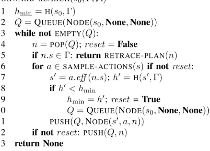
A. Forward search: persistent enforced hill-climbing Figure 2 shows a basic framework for persistent enforced hill-climbing; we use this form of search because it can maintain completeness with infinite action spaces and be-cause attempts to find a path of optimal length can quickly become bogged down with a large agenda. It is given as input an initial state s0, a set of goal constraints Γ, and a
set of possible actionsA. It keeps a queue of search nodes, each of which stores a state s ∈ S, an action a ∈ A, and a pointer to its parent node in the tree. A heuristic function
H, which we discuss in section II-C, is used to compute an estimate of the distance to reach a state satisfying Γ from state s. The search enforces hill-climbing, by remembering the minimum heuristic value hmin seen so far. Whenever
a state is reached with a lower heuristic value, the entire queue is popped, leaving only the initial state (in case this branch of the tree is a dead-end) and the current state on the queue. If the queue has not been reset, it adds the node that it just popped off back to the end of the queue. This last
FORWARD-SEARCH(s0, Γ,A)
1 hmin=H(s0, Γ)
2 Q = QUEUE(NODE(s0, None, None))
3 while not EMPTY(Q):
4 n =POP(Q); reset = False
5 if n.s∈ Γ: returnRETRACE-PLAN(n)
6 fora∈SAMPLE-ACTIONS(s) if not reset:
7 s0= a.eff (n.s); h0=H(s0, Γ)
8 ifh0< h min
9 hmin= h0; reset = True
10 Q = QUEUE(NODE(s0, None, None))
11 PUSH(Q, NODE(s0, a, n))
12 if not reset:PUSH(Q, n)
13 return None
Fig. 2: Top-level forward search.
step is critical for achieving completeness in domains with an infinite action space: it ensures that we consider taking other actions in the state associated with that node.
Intuitively, then, whenever a state with an improved heuris-tic value is reached, the queue is left containing justs0 and
the most recent state (call it s). Then, until a better state is reached, we will: sample a childs1
0 ofs0(now the queue is:
s, s1
0,s0); sample a childs1 of s (now the queue is: s10,s0,
s1,s), sample a child s(1,1)
0 ofs10 (now the queue iss0,s1,
s, s(1,1)0 , s1
0), sample a new child s20 of s0 (now the queue
is s1,s, s(1,1)
0 , s10,s20,s0), and so on. This search strategy
is as driven by the heuristic as possible, but takes care to maintain completeness through the “persistent” sampling at different levels of the search tree.
We compactly characterize the set of possible actions using action templates with the following form:
ACTIONTEMPLATE(θ1, . . . , θk):
con : (qi1, . . . , qit)∈ Ci1,...,it(θ)
...
eff : qj= ej(θ)
...
An action template specifies a generally infinite set of actions, one for each possible binding of the parametersθi,
which may be drawn from the domains of state variables or other values such as object designators. We assume that action templates are never instantiated with a set of parame-ters that violate permanent constraints (e.g., exceeding joint limits or colliding with immovable objects objects).
In addition to the heuristic, we have also left indeterminate how an action or set of actions is chosen to be applied to a newly reached state s. To do so, we must introduce the notion of a reachability graph.
B. Reachability graphs
A reachability graph (RG) is an oriented hyper-graph in which: (1) each vertex is a point in (a possibly lower-dimensional subspace of) the configuration space S, which can be represented as an assignment of values to a set of
configuration variables{Vi1= vi1, . . . , Vik = vik}; (2) each
edge is labeled with an actiona; (3) the outgoing vertices of the edge are the effects ofa; and (4) the incoming vertices of the edge are assignments that collectively satisfy the condition constraints ofa.
We say that anRGG contains a derivation of constraint C
from initial states if either (1) C is satisfied in s or (2) there exists an action a∈ G that has C as an effect and for all Ci ∈ A.con, G contains a derivation of Ci froms.
To construct the RG, we solve a version of the planning problem that is simplified in multiple ways, allowing very efficient identification of useful actions. There are three significant points of leverage: (1) individual constraints in the goal and in the conditions for an action are solved independently; (2) it is possible to plan efficiently in low-dimensional subspaces (for example, by using an RRT to find a path for the robot alone, or for an object alone); and (3) plans made in low-dimensional subspaces are allowed to violate constraints from the full space (for example, colliding with an object) and the system subsequently plans to achieve those constraints that were violated (for example, by moving the object that cause the collision out of the way).
The fundamental organizing idea is the constrained op-erating subspace(COS). A COS is a subspace of S defined by two restrictions: first, it is restricted to a set of operating constraint variables (OCV’s), and then further restricted to the intersection of that space with a set of constraintsC that are defined in terms of theOCV’s. ACOSprovides methods, used in planning, for generating potential samples in that subspace and also for generating action instances to move into and within the subspace. EveryCOSΩ is defined by:
• A setV = {Vi1, . . . , Vik} of configuration variables;
• A setC of constraints;
• An intersection sampler, which generates samples from C ∩ Ci for some domain constraint Ci of one of the
functional forms inΞ;
• A transition sampler, which generates samples (o, a, o0), where o0 =hv
i1, . . . , viki ∈ Ω, a is an action
whose effects include (but need not be limited to) Vi1 = vi1, . . . , Vik = vik, and o is an element of a
different COS.
• A roadmap sampler, which generates samples(o, a, o0) whereo∈ Ω, o0
∈ Ω, and a is an action such that the initial abstract stateo satisfies the condition constraints of a that apply to Ω’s variables and the effects of a includeo0.
Planning within a COS is completely restricted to that subspace, observing only constraints involving values of variables in V. Our definition of a COS is in contrast to Hauser’s definition of a mode, in that Hauser’s modes are defined on the complete configuration space, so that every variable either is fixed or can be controlled by the system.
In a domain with infinite state and action spaces, the corresponding RGwill generally be infinite as well. We will iteratively construct a subgraph of the fullRGthat can derive a set of goal constraintsΓ from a state s. TheRG subgraph will eventually contain actions that are the first step of a
REACHABILITYGRAPH(s, Γ) :
1 V, E ={s}, { } 2 Q = QUEUE()
3 forC∈ Γ:PUSH(Q, (C, goalSat)) GROW-RG(G, Σ, τ ) :
1 V, E = G.V, G.E; Q = V.Q; t = 0 2 while not EMPTY(Q) and t < τ :
3 C, a =POP(Q); t++
4 forΩ∈ {Ω ∈ Σ | Ω ∩ C 6= ∅}: 5 foro∈S-INTERSECTION(Ω, C) :
6 CONNECT(o, C, a); V ∪= {o}
7 V0, E0=S-TRANSITION(Ω, V ) 8 V0, E0∪=S-ROADMAP(Ω, V ∪ V0) 9 fora0∈ E0: 10 forC0∈ a0.con: 11 PUSH(Q, (C0, a0)) 12 V, E∪= V0, E0 13 PUSH(Q, (C, a))
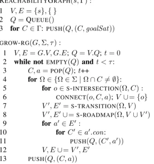
Fig. 3: Construction and growth of the reachability graph.
solution to the planning problem(s, Γ). Because it considers the satisfaction of constraints independently, it may be that there are actions that produce all of the condition constraints of some other action, but those actions are incompatible in a way that implies that this collection of actions could not, in fact, be sequenced to provide a solution. For this reason, during the forward search, we will return to the process of growing the RG, until it generates actions that are, in fact, on a feasible plan.
Procedure REACHABILITYGRAPHcreates a newRG, with start state s as a vertex (meaning that the assignment of values to variables in s can be used to satisfy conditions of edges that are added to theRG) and adds an agenda item for each constraint in the goal; these constraints are associated with the dummy action goalSat , which, when executable implies that the overall relaxed goal is satisfied.
Procedure GROWRG takes as input a partial RGG (either
just initialized or already previously partially grown), a set of COS’sΣ, and a time-out parameter τ . We assume that it, as well as all of theCOSsamplers inΣ, have a set of action templates A available to them. It grows the RG for τ steps by popping a C, a pair off of the queue, and trying to find actions that can help achieveC and adding them to the RG. It begins by generating sample elementso of the intersection between Ω and C usingS-INTERSECTION. It adds them to the set of vertices and connects them as “witnesses” that can be used to satisfy theC condition of action a. Now the transition sampler (S-TRANSITION) seeks (o, a0, o0) triples,
whereo∈ Ω, o0
∈ Ω0, ando reaches o0via actiona0. Finally,
S-ROADMAP samples(o, a0, o0) triples and adds vertices and
hyperedges that move withinΩ. Each condition of each new edge is added to the queue, and the original node is placed back in the queue for future expansion.
C. Action sampling and heuristic
Now, we can revisit the forward search algorithm in figure 2 to illustrate the points of contact with the backward algorithm. TheRG fors is first used to compute its heuristic
value. The heuristic procedure H initializes anRGfor(s, Γ) if necessary; if theRG does not yet contain a derivation for all the constraints in Γ from s, then the graph is grown in an attempt to find such a derivation. A heuristic estimate of the distance to reach Γ from s is the number of actions in a derivation. Because computing the minimum length derivation is NP-hard, we use the HFF algorithm which
greedily chooses a small derivation [23]. Because the RG
and relaxed plan graph of the HFF algorithm both make a
similar independence approximation, HFF can be computed
on top of the RG with minimal algorithmic changes. The SAMPLEACTIONS procedure seeks actions from the
RG that are applicable ins but have not yet been applied. If there are no such actions, then the RGis grown for τ steps. In our experience, it is frequently the case that as soon as a derivation is found, there is at least one action in theRGthat is feasible for use in forward search. To increase performance in practice, the first set of actions returned are restricted to the helpful actions computed by the HFF algorithm [23].
HBF can be shown to be probabilistically complete if theCOS samplers are themselves probabilistically complete. The intuition behind the argument is that the reachability graph constructs a superset of the set of solutions, due to its independence approximation. The proof is similar in nature to the probabilistic completeness proof by Hauser [4]. Due to space limitations, a sketch of this argument can be found at the following URL: http://web.mit.edu/caelan/ www/research/hbf/.
III. DOMAIN AND EXAMPLE
In this section, we describe aspects of the domain for-malization used in the experiments of the last section and work through an illustrative example. HBF is a general-purpose planning framework for hybrid domains; here we are describing a particular instance of it for mobile manipulation. Our domain includes a mobile-manipulation robot (based on the Willow Garage PR2) that can pick up, place, and push small rigid objects. The configuration spaces for prob-lem instances in this domain are defined by the following configuration variables: r is the robot’s configuration, oi is
the pose of object i, h is a discrete variable representing which object the robot is holding (its value is the object’s index or NONE), and g is the grasp transform between the held object and the gripper orNONE.
A. Action templates
The robot may move from configurationq to configuration q0 if it is not holding any object and there is a collision-free
trajectory,τ , from q to q0 given the poses of all the objects.
Each objecti also has a constraint that its pose oi be in the
set of poses that do not collide withτ . This set is represented byC-FREE-POSESi.
MOVE(q, q0, τ ):
con : r, h = q, None
oi∈C-FREE-POSESi(τ )∀i
eff : r = q0
If the robot is holding object j in grasp γ, it may move from configuration q to q0; the free-path constraint
is extended to include the held object and the effects are extended to include the fact that the pose of the held object changes as the robot moves. The values ofr and oi change
in such a way thatg is held constant. MOVEHOLDING(q, q0, τ, j, γ):
con : r, h, g = q, j, γ
oi∈C-FREE-POSES-HOLDINGi(τ, j, γ)∀i 6= j
eff : r, oj = q0,POSE(q0, γ)
The PICK action template characterizes the state change between the robot holding nothing and the robot holding (being rigidly attached to) an object. It is parameterized by a robot configuration q, an object to be picked j, and a grasp transformation γ. If the robot is in the appropriate configuration, the hand is empty, and the object is at the pose obtained by applying transformation γ to the robot’s end-effector pose when it is in configurationq, then the grasp action will succeed, resulting in objectj being held in grasp γ. No other variables are changed. The PLACEtemplate is the reverse of this action. UNSTACKand STACKaction templates can be defined similarly by augmenting PICK and PLACE
with a parameter and constraint involving the base object. PICK(q, j, γ): PLACE(q, j, γ): con : r, h = q, None oj = POSE(q, γ) eff : h, g = j, γ con : r, h, g = q, j, γ eff : h = None oj = POSE(q, γ)
The PUSH action is similar to MOVEHOLDING except that grasp transformation parameter g is replaced with an initial pose parameter p for the object. Procedure
END-POSEj computes the resulting pose of the object if the
robot moves fromq to q0 along a straight-line path.
PUSH(q, q0, j, ρ):
con : r, h, pj= q, None, ρ
oi∈C-FREE-POSES-PUSHi(q, q0, j, ρ)∀i 6= j
eff : r, oj = q0,END-POSEj(q, q0, ρ)
B. Constrained operating subspaces
Action templates define the fundamental dynamics of the domain; but to make HBF effective, we must also define the
COSs that will be used to construct RGs, selection actions, and compute the heuristic.
• Ωmove considers the robot configuration,V = {r}, and
has no constraints.
• ΩmoveHolding(i,g) is parameterized by an object i and grasp g; it considers the robot configuration and pose of object I,V = {r, oi} subject to the grasp constraint
C = {oi =POSE(r, g)}.
• Ωpush(i) is parameterized by an object i; it abstracts
away from the robot configuration and considers only the object’s pose, V = {oi}, subject to the constraint
C B A p4 p5 p6 p7 p8 p9
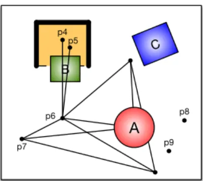
Fig. 4: An example initial state, with roadmap for objectA.
that oi ∈ table (where table is the space of poses for
oi for which it is on the table.)
• Ωplace(i) is parameterized by object i for graspable objects; it also considers only the object’s pose, V = {oi}, subject to the constraint C = {oi ∈ table}. • Ωpick(i)has the same parameters,V and C as Ωplace(i).
Each of theseCOS’s is augmented with sampling methods. Placements on flat surfaces and other objects, as well as placements in regions, are generated using Monte Carlo re-jection sampling. Inverse reachability and inverse kinematics sample robot configurations for manipulator transforms. The
S-ROADMAPsamplers for moving and moving while holding are bidirectional RRT’s that plan for the robot base then robot arm. The S-ROADMAP sampler for pushing is also a bidirectional RRT in the configuration space of just an object. Each edge of the tree is an individual push action computed by a constrained workspace trajectory planner that samples a robot trajectory that can perform the push.
C. Example
Figure 4 shows a top-down view of a table with three movable objects and a fixed u-shaped obstacle. This is the initial state s0 of a planning problem for which the goal
Γ = {oA ∈ R}, where R is the region of configuration
space for object A that would place it on the table within the fixed obstacle. Assuming that the robot is in some initial configuration q0, we can describe s0 as hr = q0, oA =
p1, oB = p2, oC = p3, h = none, g = nonei. Objects B
andC can be grasped but A cannot.
To begin the forward search, HBF must construct an initial
RG, which will be used to compute the initial heuristic value hmin and to generate the first set of actions in the search.
In the following, we will sketch the process by which the
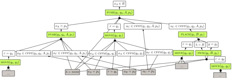
RG, G, is constructed, showing parts of G in figure 5. We adds0 to the set of vertices, add a dummy action withΓ as
its conditions constraints to the set of edges, and initialize Q = [(oA∈ R, goalSat)].
Iteration 1:C, a = (oA∈ R, goalSat) is popped from Q.
The onlyΩ that has a null intersection with C is Ωpush(A),
so V = {oA} and C = {oA ∈ table}. The first step is
to generate a set of samples of oA in R ∩ table = R;
… … … oA2 R oA= p4 r = q1 oC2 cffp(q1, q2, A, p4) oC2 cffp(q1, q2, A, p4) r = q3 oB2 cfpp(q3, q4, A, p1) oC2 cfpp(q3, q4, A, p1) oA2 cfpm(q0, q1) oA2 cfpm(q0, q1) oC2 cfpm(q0, q1) r = q5 h = B g = g1 r = q6 h = none oA= p1 r = q0 oB= p2 oC= p3 push(q1, q2, A, p4) push(q3, q4, A, p1) place(q5, B, g1) pick(q6, B, g1) move(q0, q1) move(q0, q3) move(q0, q5) move(q0, q6)
Fig. 5: Building the reachability graph.
we automatically reject sampled poses that would cause a collision with a permanent object), which we add toG. Next, we would use S-TRANSITIONto generate samples (o, a, o0);
however, because object A cannot be grasped, there are no other COSs that can be connected to Ω. Finally, we use S
-ROADMAP to generate samples (o, a, o0) that move within
Ωpush(A). This generates several more vertices, shown as
oA= p6 andoA= p7. The values ofa are complete ground
PUSH action instances; we show two particular ones (that connect up to the initial pose ofA, p1) in the figure. We add
the condition constraints of the new actions that cannot be satisfied using an existing vertex to the agenda, as well as putting the original item back on. At this point, the agenda is:[(oB∈CFPP(q1, q2, A, p4),PUSH(q1, q2, A, p4)),
(r = q1,PUSH(q1, q2, A, p4)),
(r = q3,PUSH(q3, q4, A, p1)),
(oA ∈ R, goalSat)]. (CFPP is an abbreviation for C-FREE
-POSES-PUSH.) The first constraint is that object B not be
in the way of the final push of A; the second two are that the robot be in the necessary configuration to perform each push.
Iteration 2: FromQ, we pop
C, a = (oB ∈ CFPP(q1, q2, A, p4),PUSH(q1, q2, A, p4)).
There are multipleCOSs that have non-null intersection with C, and they would each be used to generate new vertices and edges forG. In our exposition, we will focus on Ωplace(B),
so that V = {oB} and C = {oB ∈ table}. The intersection
of constraints is that oB ∈ CFPP(q1, q2, A, p4), and so we
can generate samples of poses for B that are not in the way of pushing A. Vertices like oB = p8 andoB = p9 are
added toG. Next, we useS-TRANSITIONto generate samples (o, a, o0) that connect from otherCOSs; in particular, to move in fromΩpick(B) we might sample actionPLACE(q5, B, g1)
wherep8=POSE(q5, g1). Finally,S-ROADMAP is unable to
generate samples that move within Ωplace(B). At this point,
we can add thePLACEaction toG, as well as its conditions, and add its unmet conditions to the agenda. The agenda will be augmented with ((r = q5,PLACE(q5, B, g1)), (h =
B,PLACE(q5, B, g1)), (g = g1,PLACE(q5, B, g1)).
Subsequent iterations: In subsequent iterations, an in-stance ofPICKfor objectB will be added, which can satisfy both theh = B and g = g1 conditions of thePLACE action,
and severalMOVEactions will need to be added to satisfy the robot configuration conditions. Figure 5 shows a subgraph of G containing one complete derivation of Γ. Nodes in gray with labels in them are vertices that are part of s0. Three
MOVE actions are shown with their condition constraints elided for space reasons, but they will be analogous to the one MOVE action that does have its conditions shown in detail. The green labels show the actions that are part of this derivation; there are 8 of them, which would yield an HFF
value of 8 fors0, unless there was a shorter derivation ofΓ
also contained inG. But, in fact, the shortest plan for solving this problem involves 8 steps, so the heuristic is tight in this case. Additionally, all of the actions inG whose conditions are satisfied ins0 are applied by the forward search; so all
fourMOVE actions will be considered in the first iteration.
This example illustrates the power that the RG has in guiding the forward search; the cost of computing it is non-negligible, but it is able to leverage searches in low-dimensional spaces using state-of-the-art motion-planning algorithms very effectively. Two very important things hap-pened in the process illustrated above. First, in planning how to push A into the goal region, the system was able to first reason only about the object and later worry about how to get the robot into position to perform the pushing actions. Second, it was able to plan the pushes without worrying about the fact that object B was in the way, and then later reason about how to clear the path. This style of backward goal-directed reasoning is very powerful and has been used effectively to solve NAMO (navigation among movable obstacle) problems [24] and by the HPN
planner [18].
IV. EXPERIMENTAL RESULTS
We applied HBF to six different manipulation problems to characterize its performance. The planner, samplers, and PR2 robot manipulation simulations were written in Python using
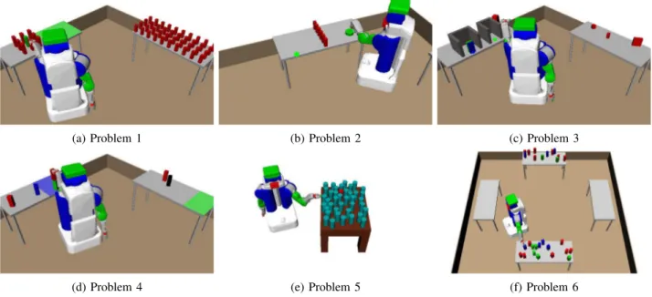
(a) Problem 1 (b) Problem 2 (c) Problem 3
(d) Problem 4 (e) Problem 5 (f) Problem 6
Fig. 6: An early state on a valid plan for each problem.
P H0 HFF
% runtime length visited % runtime length visited 1 100 12 (7) 8 (0) 156 (140) 100 4 (1) 12 (2) 6 (2) 2 97 62 (26) 16 (0) 208 (37) 100 7 (1) 16 (0) 10 (1) 3 62 238 (62) 16 (0) 2315 (712) 100 6 (1) 16 (0) 37 (2) 4 0 300 (0) - (-) 1293 (93) 97 12 (4) 24 (4) 56 (24) 5 0 300 (0) - (-) 1591 (381) 98 23 (9) 24 (4) 85 (37) 6 0 300 (0) - (-) 637 (40) 100 82 (13) 72 (4) 191 (37)
Fig. 7: Manipulation experiment results over 60 trials.
Fig. 8: Problem 6 HFF runtimes.
OpenRAVE [25] without substantial performance optimiza-tion. In each problem, red objects represent movable objects that have no specified goal constraints. However, they impose geometric constraints on the problem and must usually be manipulated in order to produce a satisfying plan.
Problem 1: The goal constraint is for the green block, which is surrounded by 8 red blocks, to be on the green region on the table. Notice that the right table has 40 movable red objects on it that do not block the path of the green object. Problem 2: The goal constraint is for the green cylinder to be at the green point on the edge of the table. The cylinder is too big for the robot to to grasp, so it must push it instead. The robot must move several of the red objects and then push the green cylinder several times to solve the problem.
Problem 3: A thin but wide green block starts behind a similar blue block. The goal constraints are that the green block be at the green point and that blue block be at the blue point, which is, in fact, its initial location. The is problem is non-monotonic in that the robot must first violate one of the goal constraints, and then re-achieve it. Additionally, the right cubby housing the green goal point is thinner than the left cubby, so the green block can only be placed using a subset of its grasps, all of which are infeasible for picking it
up at its initial location. This forces the robot to place and regrasp the green block.
Problem 4: The goal constraints are that the green block be on the green region of the table, the blue block be on the blue region of the table, and the black block be on top of the blue block. Because the black block must end on the blue block, which itself must be moved, no static pre-sampling of object poses would suffice to solve the problem. Additionally, a red block starts on top of the green block, preventing immediate movement of the green block.
Problem 5: This is exactly the same problem considered by Srivastava et al. [7]. The goal constraint is to be holding the red cylinder with an arbitrary grasp. 39 blue cylinders crowd the table, blocking the red object.
Problem 6: The goal constraints are that all 7 blue blocks must be on the left table and all 7 green blocks must be on the right table. There are also 14 red blocks. The close proximity of the blocks forces the planner to carefully order its operations as well as to move red blocks out of the way. Solutions: The planner uses the same set of sampling primitives on each problem with no problem-dependent information. Each object has a possibly infinite number of grasps, computed from its geometry. However, the first four generated are typically sufficient to solve the problems
posed here. We restrict the PR2 to side grasps to highlight the constrained nature of manipulation with densely packed objects.
We compared the performance of HBF when H= HFF to
the performance of an unguided version where H(s) = 0 for all s. We enforce a five-minute timeout on all experiments. There were 60 trials per problem all conducted on a laptop with a 2.6GHz Intel Core i7 processor. Each entry in figure 7 reports the success percentage (%) as well as the median and median absolute deviation (MAD) of the runtime, resulting plan length in terms of the number of actions, and number of states visited in the forward search. The median-based statistics are used to be robust against outliers. Figure 8 shows the distribution of runtimes for HFF on problem 6.
Several outliers cause the mean runtime of 93 (the red line) to be larger than the median runtime (the green line). The statistics for trials that failed to find a solution are included in the entries. Thus, entries with a runtime of 300 and MAD of 0 did not find a plan for any trial. The accompanying video simulates the PR2 executing a solution found by HBF for each problem.
Both versions of HBF solve problem 1 in several seconds despite the extremely high-dimensional configuration space. A manipulation planning algorithm that explores all adjacent modes [3], [4] would be overwhelmed by the branching factor despite the otherwise simple nature of the problem. The unguided search was unable to solve problems 4, 5, and 6 in under 5 minutes due to the size of the constructed state space and planning horizon. On problem 5, Srivastava et al. report a 63 percent success rate (over randomly generated initial conditions) with an average runtime of 68 seconds. The median runtime of HBF is about a third of the Srivastava et al. runtime with a 98 percent success rate. Problem 6 is comparable in nature to but more complex than task 5 considered in FFRob [20]. Additionally, the runtime is about half the FFRob reported median runtime of 157 seconds.
Conclusions: The experiments show that by leveraging the factored nature of common manipulation actions, HBF is able to efficiently solve complex manipulation tasks. The runtimes are improvements over runtimes on comparable problems reported by Srivastava et al. and Garrett et al. [20], [7]. Additionally, the dynamic search allows HBF to solve regrasping, pushing, and stacking problems all using the same planning algorithm. These results show promise of HBF scaling to the large and diverse manipulation problems prevalent in real world applications.
REFERENCES
[1] T. Sim´eon, J.-P. Laumond, J. Cort´es, and A. Sahbani, “Manipulation planning with probabilistic roadmaps,” IJRR, vol. 23, pp. 729–746, 2004.
[2] S. Cambon, R. Alami, and F. Gravot, “A hybrid approach to intricate motion, manipulation and task planning,” International Journal of Robotics Research, vol. 28, 2009.
[3] K. Hauser and J. Latombe, “Integrating task and prm motion planning: Dealing with many infeasible motion planning queries,” in ICAPS09 Workshop on Bridging the Gap between Task and Motion Planning, 2009.
[4] K. Hauser and V. Ng-Thow-Hing, “Randomized multi-modal motion planning for a humanoid robot manipulation task,” IJRR, vol. 30, no. 6, pp. 676–698, 2011.
[5] M. R. Dogar and S. S. Srinivasa, “A planning framework for non-prehensile manipulation under clutter and uncertainty,” Auton. Robots, vol. 33, no. 3, pp. 217–236, 2012.
[6] J. Barry, L. P. Kaelbling, and T. Lozano-Perez, “A hierarchical approach to manipulation with diverse actions,” in Robotics and Automation (ICRA), 2013 IEEE International Conference on. IEEE, 2013, pp. 1799–1806.
[7] S. Srivastava, E. Fang, L. Riano, R. Chitnis, S. Russell, and P. Abbeel, “Combined task and motion planning through an extensible planner-independent interface layer,” in IEEE Conference on Robotics and Automation (ICRA), 2014.
[8] T. Lozano-P´erez, “Automatic planning of manipulator transfer move-ments,” IEEE Transactions on Systems, Man, and Cybernetics, vol. 11, pp. 681–698, 1981.
[9] T. Lozano-P´erez, J. L. Jones, E. Mazer, P. A. O’Donnell, W. E. L. Grimson, P. Tournassoud, and A. Lanusse, “Handey: A robot system that recognizes, plans, and manipulates,” in IEEE International Con-ference on Robotics and Automation, 1987.
[10] G. T. Wilfong, “Motion planning in the presence of movable obsta-cles,” in Symposium on Computational Geometry, 1988, pp. 279–288. [11] R. Alami, T. Simeon, and J.-P. Laumond, “A geometrical approach to planning manipulation tasks. the case of discrete placements and grasps,” in ISRR, 1990.
[12] R. Alami, J.-P. Laumond, and T.Sim´eon, “Two manipulation planning algorithms,” in WAFR, 1994.
[13] C. Dornhege, P. Eyerich, T. Keller, S. Tr¨ug, M. Brenner, and B. Nebel, “Semantic attachments for domain-independent planning systems,” in International Conference on Automated Planning and Scheduling (ICAPS). AAAI Press, september 2009, pp. 114–121.
[14] C. Dornhege, A. Hertle, and B. Nebel, “Lazy evaluation and subsump-tion caching for search-based integrated task and mosubsump-tion planning,” in IROS workshop on AI-based robotics, 2013.
[15] E. Erdem, K. Haspalamutgil, C. Palaz, V. Patoglu, and T. Uras, “Combining high-level causal reasoning with low-level geometric reasoning and motion planning for robotic manipulation,” in IEEE International Conference on Robotics and Automation (ICRA), 2011. [16] F. Lagriffoul, D. Dimitrov, A. Saffiotti, and L. Karlsson, “Constraint propagation on interval bounds for dealing with geometric backtrack-ing,” in IEEE/RSJ International Conference on Intelligent Robots and Systems (IROS), 2012.
[17] E. Plaku and G. Hager, “Sampling-based motion planning with sym-bolic, geometric, and differential constraints,” in IEEE International Conference on Robotics and Automation (ICRA), 2010.
[18] L. P. Kaelbling and T. Lozano-Perez, “Hierarchical planning in the now,” in IEEE Conference on Robotics and Automation (ICRA), 2011. [19] A. K. Pandey, J.-P. Saut, D. Sidobre, and R. Alami, “Towards planning human-robot interactive manipulation tasks: Task dependent and human oriented autonomous selection of grasp and placement,” in RAS/EMBS International Conference on Biomedical Robotics and Biomechatronics, 2012.
[20] C. R. Garrett, T. Lozano-P´erez, and L. P. Kaelbling, “Ffrob: An efficient heuristic for task and motion planning,” in International Workshop on the Algorithmic Foundations of Robotics (WAFR), 2014. [21] B. Bonet and H. Geffner, “Planning as heuristic search: New results,” in Proc. of 5th European Conf. on Planning (ECP), 1999, pp. 360–372. [22] ——, “Planning as heuristic search,” Artificial Intelligence, vol. 129,
no. 1, pp. 5–33, 2001.
[23] J. Hoffmann and B. Nebel, “The FF planning system: Fast plan generation through heuristic search,” Journal Artificial Intelligence Research (JAIR), vol. 14, pp. 253–302, 2001.
[24] M. Stilman and J. J. Kuffner, “Planning among movable obstacles with artificial constraints,” in Proceedings of the Workshop on Algorithmic Foundations of Robotics (WAFR), 2006.
[25] R. Diankov and J. Kuffner, “Openrave: A planning architecture for autonomous robotics,” Robotics Institute, Carnegie Mellon University, Tech. Rep. CMU-RI-TR-08-34, 2008.