Balancing product flow and synchronizing transportation

Balancing Product Flow and Synchronizing Transportation

Priya Andleigh

Bachelor of Engineering, Chemical and Biomolecular Engineering, Nanyang Technological University, 2013

and

Jeffrey Scott Bullock

Bachelor of Science, Manufacturing Engineering Technology, Brigham Young University, 2012

SUBMITTED TO THE PROGRAM IN SUPPLY CHAIN MANAGEMENT IN PARTIAL FULFILLMENT OF THE REQUIREMENTS FOR THE DEGREE OF

MASTER OF ENGINEERING IN SUPPLY CHAIN MANAGEMENT AT THE

MASSACHUSETTS INSTITUTE OF TECHNOLOGY JUNE 2017

@ 2017 Priya Andleigh and Jeffrey Scott Bullock. All rights reserved.

The authors hereby grant to MIT permission to reproduce and to distribute publicly paper and electronic copies of this thesis document in whole or in part in any medium now known or hereafter created.

Signature of Author... Ma Signature of Author... Certified by... Certified by...

S

c~' :

AUG 0 12011

Signature redacted

ster of Engineering in Supply Chain Management Program

Signature

redacted

ster of Ah ineering in Supply Chain Management Program

Signature redacted

... ... .... .... .... .... .. ... ... . Dr. Ahmad Hemmati Postdocto s 9 Center forT sport & Logistics

ianature redacted

...

ov .Dr. Chris Caplice Executive Director, Center for Transportation & Logistics

I T

.~.. .jThesis Supervisor

oiyiLuIu

IeUdL LeU

co

wJ

0~

{

...

Balancing Product Flow and Synchronizing Transportation by

Priya Andleigh and

Jeffrey Scott Bullock

Submitted to the Program in Supply Chain Management on May 12, 2017 in Partial Fulfillment of the

Requirements for the Degree of

Master of Engineering in Supply Chain Management

ABSTRACT

Traditionally, production and transportation planning processes are managed separately in organizations. In such arrangements, order processing, load planning, and transportation scheduling are often done sequentially, which can be time consuming. Establishing a proactive steady flow of products between two nodes of a supply chain can bypass this order-plan-ship process. A steady flow of products can reduce transportation costs, increase cross-dock productivity, and reduce bullwhip effect upstream in the supply chain. This thesis develops an analytical framework to calculate this steady flow. The determination of eligible SKUs in this approach is performed by analyzing each SKU's historical and forecasted demand. The level of flow of each SKU is found using optimization with the objective of maximizing total savings. The methodology was tested on a plant-to-warehouse lane of a fast moving consumer goods company. The relationship between demand characteristics and optimal steady flow was studied. It was found that as the coefficient of variation decreases, the optimum steady flow moves closer to the mean of the non-zero demand and selected forecast over the model horizon. The methodology developed in the research, with its potential to reduce transportation cost and improve warehouse productivity, also presents the opportunity for new and innovative contract types with transportation providers.

Thesis Supervisor: Dr. Ahmad Hemmati

Title: Postdoctoral Associate, Center for Transportation & Logistics Thesis Supervisor: Dr. Chris Caplice

Acknowledgements

We would like to extend our sincere gratitude to Dr. Ahmad Hemmati and Dr. Chris Caplice for their guidance and expertise on this subject and to the Sponsor Company and affiliated partners for their valuable inputs that helped shape this thesis.

A special thanks to our colleagues and industry experts for their insights and to our friends and family for their unconditional support.

Table of Contents

1. Introduction ... 6

2. Literature Review ... 8

2.1. Steady Product Flow ... 8

2.2. Transportation Selection ... ₉

2.3. Literature Review Conclusion... 10

3. M ethodology and Analysis...11

3.1. Business Context... 11

3.2. M odel Fram ework ... 12

3.2.1. SKU Eligibility... 14

3.2.2. Steady Flow Calculation ... 16

3.2.3. Final SKU Selection ... 24

3.3 Param eter Tuning... 27

4. Results and Discussion... 28

4.1. Test Lane Results... 28

4.1.1. Effect of SKU Characteristics on Steady Flow ... 28

4.1.2. Effect of Param eters on M odel Performance ... 32

4.2. Assum ptions and Lim itations ... 37

4.2.1. Data Aggregation... 38

4.2.2. Vehicle Capacity Utilization ... 38

4.2.3. Other Cost Considerations ... 39

4.2.4. Forecast Accuracy... 40

4.2.5. Distribution Resource Planning (DRP)... 41

4.2.6. Segm entation of Dem and ... 42

4.3. Im plications ... 43

4.3.1. Bullw hip Dam pening ... 43

4.3.2. Transportation Contract Innovation ... 44

4.3.3. Applicability ... ₄₄

List of Figures

Figure 3-1 Steady Flow Calculation Fram ework... 12

Figure 3-2 Savings and Cost Tradeoffs as Steady Flow Quantity of Pallets Increases for a sample SKU.. 16

Figure 3-3 Cross-dock savings are calculated using a minimum of demand and steady flow...18

Figure 3-4 Accumulation of excess inventory when demand is lower than steady flow...20

Figure 4-1 Dem and and Steady flow for SKU A... 29

Figure 4-2 Effect of change in steady flow on total costs for SKU A ... 30

Figure 4-3 Demand and Steady Flow for high COV SKU B ... 31

Figure 4-4 Effect of change in steady flow on total costs for SKU B ... 31

Figure 4-5 Effect of length of history on actual savings and estimated savings accuracy...33

Figure 4-6 Effect of length of forecast on actual savings and estimated savings accuracy ... 34

Figure 4-7 Effect of change of threshold coefficient of variation of demand on actual savings and estim ated savings accu racy ... 35

Figure 4-8 Effect of change of threshold % of weeks with demand on actual savings and estimated sav ing s accu racy ... 3 6 Figure 4-9 Effect of change of threshold % forecast weeks with non-zero forecast on actual savings and estim ated savings accuracy ... 37

List of Tables

1. Introduction

A major percentage of any shipper's budget is allocated to inventory holding costs and transportation costs. One of the goals of a shipper is to reduce the overall spend on these activities every year. Products flow through any shipper's network based on customer demand. For any given product, that

demand typically fluctuates over time. Many Stock Keeping Units (SKUs) may be fast-moving and always have demand, whereas other SKUs may have more sporadic demand cycles.

When a product's demand is higher, and more frequent, that product is shipped consistently. Instead of waiting for orders to be placed, would it be beneficial to ship a certain amount of the expected

demand for that product proactively? Both financial benefits and risks are associated with setting up this type of distribution structure. Currently, little research has been done in this area to determine

eligible SKUs or provide optimal levels of steady flow for each SKU. The focus of this thesis is to provide an analytical framework to close that gap and maximize the benefits while minimizing the risks. Some benefits include shorter lead-times, decreased transportation costs, and warehouse cross-docking.

The major risk is the potential to increase inventories and consequently the inventory holding costs. To take advantage of the savings while managing the risks, the framework determines which SKUs are

eligible and how much of each SKU should be shipped proactively.

The determination of eligible SKUs is performed by analyzing each SKU's historical and forecasted demand. Key descriptive statistic measures, such as coefficient of variation of demand, percentage of non-zero forecast, and percentage of time-periods with non-zero demand are used as the eligibility

criteria. Each SKU's level flow is calculated so that the total savings is maximized. The collection of eligible SKUs is then further optimized taking into consideration vehicle capacity utilization. This

analytical framework can enable a shipper to reduce inventory levels, increase cross-dock

productivity, increase vehicle capacity utilization, and reduce overall transportation spend.

This thesis first presents a review of existing literature around steady flow and associated cost savings

in Chapter 2. Chapter 3 provides a business context and details the analytical framework developed in this research. Chapter 4 presents the results of testing the methodology on a plant-to-warehouse lane and discusses the assumptions, limitations, and implications of the research.

2. Literature Review

The focus of this thesis project is determining an optimal mix of SKUs as well as finding the optimal

quantity of each to ship proactively. This section first reviews the lean methodology of steady production flow. Then it focuses on the approaches used in the industry to utilize the most

appropriate transportation modes and methods. Further, it reviews existing literature, discussing the impact of balancing product flow on transportation costs and contracts. Finally, it discusses the gaps

that this thesis fills.

2.1. Steady Product Flow

Leveling production flow is a lean principle, which can lead to significant cost savings. Two key success drivers in implementing level production flow in a plant are the synchronization of raw

materials planning and lot size determinations (Deif & ElMaraghy, 2014). Leveling production flow has been studied in detail, but leveling the flow of products (steady product flow) between nodes

of the supply chain has not received as much attention. This thesis addresses the question of which products are eligible for steady flow and what their appropriate steady flow quantities should be.

A steady product flow implementation can have many benefits. An increase in overall shipment reliability is a major benefit to shippers and distributors when faced with supply chain disruptions (Riessen et al., 2015). Also, cross-docking has been a strategy for a lot of companies to reduce warehouse space and reduce overall inventory (Kulwiec, 2004). Cross-dock productivity is

product flow, a shipper can decrease inventory dwell time as well as transportation cycle time, and thus increase cross-docking opportunities.

2.2. Transportation Selection

If level product flow is implemented between nodes of the supply chain, then level transportation flow is required to support it. A lot of research has been conducted in the optimization of multiple modes of transportation on a single lane. Despite this, the diversity in mode utilization is lower in practice, and implementation of a more synchronized transportation model could offer shippers better cost and service opportunities (Behdani, Fan, Wiegmans, & Zuidwijk, 2016). Cooperation among all parties in the supply chain is required to ensure success in implementing a synchronized

framework (Pfoser, Treiblmaier, & Schauer, 2016).

In addition to modes of transportation, the balancing of long-term and short-term contract types can yield strategic benefits. Research to determine the best mix of contract types (fixed volume

vs. on-demand volume) was conducted and analyzed for appropriate implementation (van Duin, Tavasszy, & Taniguchi, 2007). Van Duin et al. determined that spot markets could oftentimes produce cheaper transportation costs depending on the bid method utilized due to the wide

variety of carrier options. Spot bids can be lower due to a carrier's need to move equipment full or empty along the shipper's desired lane (Garrido, 2007). Further analysis was performed to find

the best bid methods in the often capacity-starved spot bid market (Lindsey & Mahmassani, 2016). However, van Duin et al. concluded that the benefits of guaranteed capacity in fixed contracts with a smaller group of core carriers could actually reduce overall costs in the long run. It is also possible to find savings by structuring a flexible contract which includes fixed capacity as

well as additional potential capacity with individual carriers (Zhelev, 2001). This project will build

upon these research findings by using demand characteristics and business requirements to drive and adapt the optimal mix and level of contract types.

2.3. Literature Review Conclusion

The existing research has focused primarily on optimizing transportation modes based on mode

availability and pricing. There has been much discussion regarding different contract structures and how to build relationships with a network of carriers. The impact of a synchronized level flow of products on downstream metrics has been analyzed. This thesis project seeks to bridge these

topics and create an overarching model that incorporates them all into one framework. In addition, this project also analyzes demand patterns and identifies specific SKUs that would be

optimal candidates for level product flow. Such a framework that identifies a specific set of SKUs will allow shippers to bridge the gap from theory to implementation.

3. Methodology and Analysis

3.1. Business Context

The research of this thesis was conducted in the context of a fast moving consumer goods

company with a wide range of products. Plants typically manufacture one or more categories of products and ship to a network of regional warehouses. A single warehouse receives products

from multiple plants and further ships the product to customers.

Traditionally, the production and transportation planning processes are managed separately in most companies (Pirkul & Jayaraman, 1996). Most commonly, shipment of products from the

plant to the warehouse entails three activities: order, plan, and ship. The warehouse places an order to the plant for products in accordance with actual customer orders as well as forecasted

demand. The placing of an order triggers the load planning or load building process that entails deciding which SKUs should be placed on a single truck constrained by weight and volume limitations. After load planning is completed, the shipment process begins. Transportation

carriers are then contacted to request for required capacity. Upon acceptance of the load by a carrier, load pick-up planning is done. Subsequently, the load is picked up and transported to the

warehouse.

The time lag from the beginning of the process to load pick-up depends on the speed of the order-plan-ship process. This research aims to eliminate this time lag by proposing a "steady flow" of

products from the plant to the warehouse on a regular basis. Setting a regular shipment has the potential to reduce total transportation costs, increase warehouse productivity via cross-docking

products directly to customer orders, and bring stability to the system through higher predictability. The focus of this research is to build an analytical framework to determine the optimal "steady flow" of products.

3.2. Model Framework

To begin building an analytical framework, one specific lane was chosen to study and test. The

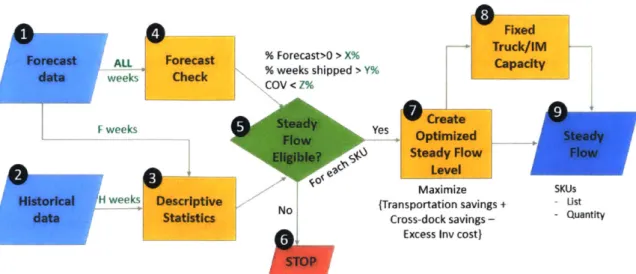
focus of this study is a plant-to-warehouse lane. An intra-company lane such as this was chosen because a single company would have more independence changing its shipment strategy as compared to an external lane involving two or more companies. To determine the optimal steady flow on the plant-to-warehouse lane, the demand data from the warehouse out to the customers was utilized. This data was aggregated to a weekly level, and the unit of measure for time used in this model was a week. The overall approach that was developed to determine the steady flow is

shown in Figure 3-1.

ALL Foecast % Forecast>O > X%

we s Foecst % weeks shipped > Y9i

cov < Z% weeks Steady - Flow Eligible? weeks Descriptive Statistics No Fixed Truck/IM Capacity Create es Optimized Steady

Steady Flow Flow

Level

Maximize SKUs

(Transportation savings + - Ust

cross-dock savings - - Quantity

Excess Inv cost}

Figure 3-1 - Steady Flow Calculation Framework

0

Forecast

0

Historical H data

The process is as follows. Starting in boxes 1 & 2 (Figure 3-1), SKU level forecast and historical data

are used to characterize the demand. First, descriptive statistics (box 3) of the demand are calculated. In order to do this, a determination needs to be made as to how much data would be

used for these calculations. In other words, how many weeks of historical data (say, H weeks) and forecast data (say, F weeks) should be used? The number of weeks for each are input parameters that can be tuned. The calculated statistics from the specified timeframe (H weeks + F weeks, henceforth called "model horizon") include mean of demand, standard deviation of demand, coefficient of variation (COV) of demand, minimum demand, as well as percentage of weeks with demand (non-zero values). Only weeks with demand (non-zero values) are used to calculate the

mean, standard deviation, COV, and minimum demand to ensure the statistics were not affected by weeks without shipments. Next, a forecast check is performed (box 4) by analyzing the full length of available forecast data to determine the percentage of forecast weeks with a non-zero

demand. This check is performed to filter out any SKUs that are being phased out of production.

These summary statistics are then used to determine whether the SKU is eligible for steady flow (box 5). Eligibility is discussed in further detail in Section 3.2.1. If the SKU is found to be ineligible,

it is marked as such and disregarded (box 6). If a SKU is found to be eligible, its optimal steady flow is then calculated (box 7). The optimal steady flow is chosen by maximizing total savings, which includes transportation savings, cross-dock savings, and cost of excess inventory. The

mathematical calculations of steady flow are presented in detail in Section 3.2.2. Optimal steady flow is calculated for every eligible SKU. An optimization is then performed to select the best mix of SKUs that maximizes total savings while conforming to a minimum vehicle capacity utilization

constraint. This collection of SKUs and their corresponding quantities for steady flow is the model's final output and recommendation (box 9).

The first six months of weekly steady flow is studied to calculate the average and minimum number of trucks/containers required for the steady flow of products. Once the steady flow of

containers is determined, it is used as an additional constraint in the final SKU selection process

(box 8). Details of the final SKU selection process are discussed in Section 3.2.3.

Since the weekly forecast data is being used, the model was designed to be utilized once every

week. Ideally, if the total savings or SKU mix on the steady flow does not change beyond a certain tolerance set by the organization, the steady flow should remain constant week after week. Changing the steady flow every week would incur additional time and effort to plan the containers

as opposed to longer time intervals. However, this would still result in a reduction in time and effort compared to the current load planning, which is performed on a daily basis using the

traditional order-plan-ship process. Further details of SKU eligibility, steady flow calculation, and final SKU selection are presented in the sections below.

3.2.1. SKU Eligibility

Identifying SKUs that are eligible for steady flow is an important step to ensure longer-term

validity of the flow. The purpose of this step is to filter out SKUs that the company will discontinue in the near future, that are shipped sporadically, or that have very high variance in shipment volumes. The model uses three criteria to test the eligibility of the SKUs for steady flow: percentage of forecast weeks with non-zero forecast, percentage of weeks with

demand, and coefficient of variation of demand. These three criteria were selected because they describe the frequency and variation of demand over the model horizon. Each of the

criteria are described below:

i. Percentage of forecast weeks with non-zero forecast:

SKUs in every industry have a lifecycle. SKUs enter the market, vary in demand, and many are eventually phased out. In order to make sure that discontinued SKUs are not added to the steady flow, a forecast check is applied. This check calculates the percentage of weeks in the total forecast length where the expected demand was non-zero. If this percentage fails to meet the threshold set by the user, the SKU is labeled ineligible.

ii. Percentage of weeks with demand:

Even if a SKU remains in the portfolio of the company for a long period of time, there may be some SKUs that only ship regularly during a certain season, or others that are

slow-moving and have sporadic demand. The percentage of weeks in the model horizon that have a non-zero demand is calculated and compared against the threshold set by the user.

Any SKUs being demanded less frequently than pre-determined user tolerance are labeled as ineligible for steady flow.

iii. Coefficient of variation (COV) of demand:

This check is designed to limit steady flow to SKUs that do not have large variations in demand over the model horizon. Only weeks in the model horizon that had a non-zero demand were included in the calculation of the COV. The upper limit for an approved COV

The above eligibility criteria were created as input parameters to the model so that they could be changed to align with time-relevant business decisions.

3.2.2. Steady Flow Calculation

If a SKU is determined to be eligible for steady flow, its optimal steady flow quantity is then

determined. The objective of the optimization is to determine the quantity of each given SKU that should be put on steady flow that would maximize the total savings.

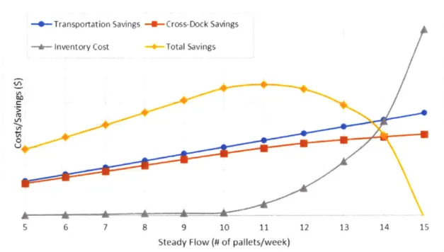
The trade-off between transportation savings, cross-dock savings, and excess inventory costs is the primary driver of the optimization. Figure 3-2 illustrates this trade-off as the steady flow quantity of pallets increases for a sample SKU. Each of these savings and costs are described below.

-4--Transportation Savings -4-Cross-Dock Savings -e- Inventory Cost -4-Total Savings

5 6 7 8 9 10 11 12 13 14 15

Steady Flow (# of pallets/week)

Transportation Savings:

As noted in Section 2.2, fixed volume transportation contracts can help shippers negotiate a better price with carriers. These savings per container (or truck) are used in the model

to calculate total transportation savings. All pallets on the steady flow contribute to the transportation savings. Transportation savings is calculated as follows:

n

Transportation savings = (s

**

i=1

Definitions (units)

n = # weeks in model horizon (weeks)

s = number of pallets on steady flow (pallet)

j

The # of weeks in the model horizon, n, is found by adding the total number of historical and forecast weeks used. By definition, the steady flow "s" remains constant for the model horizon. The percentage of a truckload (% TL) that each pallet represents is found

by averaging the % TL by weight with the % TL by cube. This calculation provides a more accurate percentage of a truckload for each pallet because it considers vehicle capacity

utilization. The transportation savings per truck, p, is the cost reduction from establishing a fixed-volume contract with a carrier and will vary by lane.

ii. Cross-Dock Savings:

A steady flow between the plant and warehouse opens the possibility of synchronizing

the arrival of products at the warehouse with their scheduled loading for customer shipment. This cross-docking can help reduce storage and logistics costs at the warehouse and increase productivity.

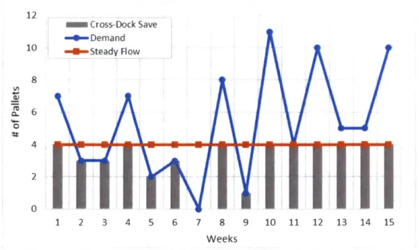
It is possible to achieve cross-dock savings, as long as the steady flow is lower than the demand for that week. If the demand is lower than the steady flow quantity, only the demand quantity is available to be cross-docked. Figure 3-3 illustrates this concept. In week 1, the sample SKU's demand is higher than the steady flow. As such, all 4 units of steady flow can be cross-docked. However, for week 2, since the demand (3 pallets) is lower than the steady flow (4 pallets), only 3 pallets of the SKU can be cross-docked that week. 12 12Cross-Dock Save - Demand 10 - Steady Flow 8 4 0

0

Moreover, not all pallets on steady flow may be eligible to be cross-docked due to factors other than lack of demand, such as a delay in the outbound carriers, change in supply volumes to customers, warehouse limitations, customer logistics delays, etc. Thus, a cross-dock eligibility factor, ce, is included in the calculation. This factor, ce, can range

from 0 to 1. A ce value of 1 indicates that all pallets on the steady flow can be

cross-docked, while a value of 0 indicates that none of the pallets on the steady flow are eligible for cross docking. Ce is an input parameter that is user-defined in accordance with the

company's business processes. It can be found based on the lead-time required to estimate actual cross-dock activities that can truly be realized while utilizing the steady

flow.

Cross-dock savings is calculated as follows:

n

Crossdock savings = Min(s, di) * C* Ce

i=1

Definitions (units)

n = # weeks in model horizon (weeks)

s = number of pallets on steady flow (pallet)

di= demand for week i (pallet)

Cs = cross-dock savings per pallet ($/pallet)

Ce = cross-dock eligibility: 0 5 ce 1 (dimensionless)

The # of weeks in the model horizon, n, is found by adding the total number of historical and forecast weeks used. By definition, the steady flow "s" remains constant for the

model horizon. c, and ce are also user-defined parameters based on the company's business processes.

iii. Excess Inventory Cost:

SKUs on the steady flow ship regularly from the plant to the warehouse. Due to inherent variation in demand, in some cases, the number of pallets of a SKU on the steady flow will exceed the demand. This could lead to a build-up of inventory at the warehouse until the demand in the next period(s) is able to absorb the excess inventory. To account for this, excess inventory cost is considered. Figure 3-4 illustrates the concept of inventory build-up in cases where demand is lower than steady flow in certain weeks.

12 12Excess Inventory -1- Demand 10 -0--Steady Flow 8 6

Yv A

I

A

1

Figure 3-4 -Accumulation of excess inventory when demand is lower than steady flow

As seen in Figure 3-4, when the steady flow is lower than the demand (week 1), there is no excess inventory. In week 2, the demand (3 pallets) falls below the steady flow of 4

pallets. Thus, excess inventory of 1 pallet is accumulated in the warehouse. This is carried to week 3. The demand for week 3 is again lower than the steady flow, thus contributing

one additional pallet to the excess inventory. The two pallets of excess inventory are then carried to week 4. However, the demand in week 4 is higher than the steady flow by 3 pallets. Thus, the inventory being carried over is used up in week 4 and no excess is carried forward to week 5, and so forth.

Excess inventory cost is calculated as follows:

Excess Inventory Cost = Max((e _ + s - di),0) *j * h * v}

Definitions (units)

n = # weeks in model horizon (weeks)

e1_1 = excess inventory running total in week i-1; eo = 0 (pallet) s = number of pallets on steady flow (pallet)

di = demand for week i (pallet)

j

h = inventory holding cost ($/$/weeks)

v = inventory value ($/truck)

The # of weeks in the model horizon, n, is found by adding the total number of historical and forecast weeks used. By definition, the steady flow "s" remains constant for the

by averaging the % TL by weight with the % TL by cube. This calculation provides a more accurate percentage of a truckload for each pallet because it considers vehicle capacity utilization. The inventory holding cost, h, and the inventory value, v, are both user-defined

parameters based on the company's business processes and product characteristics. In

addition to the above, excess inventory left over at the end of the model horizon (i = n) is

subject to an end-of-period penalty.

End of Period Penalty = {Max((en- ₁ + s - dn), 0) *] * t * r)

Definitions (units)

r = end of period risk factor (%)

The end of period risk factor, r, is the percentage chance that the excess inventory remaining at the end of the period remains indefinitely. In other words, r represents the

associated risk that a SKU on steady flow will be phased out before the excess inventory can be dispersed.

By combining the above, the total excess inventory cost is calculated as follows:

Excess Inv Cost

= Max((e1, + s - di),0)

*j

+ {Max((en_₁ + s - d), 0)

*1

Total Savings = Transportation Savings + Crossdock Savings - Excess Inv Cost

As the steady flow increases, transportation cost savings increase, cross-dock savings increase (until steady flow exceeds demand), but at the same time excess inventory costs also increase. Thus, there exists a point that maximizes the total savings before excess inventory costs catch

up with the transportation and cross-dock savings.

The mathematical formulation of the optimization is summarized as follows:

Total Savings = Transportation Savings + Crossdock Savings - Excess Inv Cost Objective function: MAXIMIZE Total Savings

Decision Variable: Number of Pallets on Steady Flow (s)

n

Transportation savings = (S*

j

i=1

n

Crossdock savings = Min(s, di) * cs * ce

i=1

Excess Inv Cost

= Max((e,- + s - di),0) * j * h * v

+ {Max((en-1 + s - d), 0) * j * v * r} Definitions (units)

n = # weeks in model horizon (weeks)

s = number of pallets on steady flow (pallet)

p = transportation savings per truck ($/truck)

di= demand for week i (pallet)

c= cross-dock savings per pallet ($/pallet)

Ce = cross-dock eligibility: 0 5 ce 1 (dimensionless)

ei_1 = excess inventory running total in week i-1; eo = 0 (pallet)

h = inventory holding cost ($/$/weeks)

v = inventory value ($/truck)

r = end of period risk factor (%)

In the model, the above optimization is performed for each SKU by using the hill-climbing

technique. This technique was used to minimize the model's calculation runtime. It calculates the savings with an initial steady flow value equal to the minimum pallets of demand. It then increases the number of pallets on steady flow until the point where savings start to decline.

Thus, the maximum savings is found and the corresponding number of pallets is set as the steady flow amount.

This process is repeated for all SKUs that are found to be eligible for steady flow.

3.2.3. Final SKU Selection

After the list of SKUs eligible for steady flow and their corresponding optimal steady flow quantity are determined, truck/container weight and volume constraints are taken into consideration. First, the total number of trucks represented by a given SKU, both based on weight and volume are calculated. For dense products, the number of trucks required on the

basis of weight may be higher than that on the basis of volume. Conversely, for light products, the number of trucks required by volume may exceed the number of trucks required by

weight. Collectively, for all steady flow eligible products, the model then optimizes the combination of heavy and light products to maximize savings in accordance with vehicle capacity utilization requirements.

Vehicle capacity utilization, also referred to as vehicle fill rate, is the ratio of utilized vehicle capacity to available vehicle capacity. Depending on the density of the products, a vehicle may reach the maximum allowed weight (weighed-out) before reaching the maximum allowed volume (cubed-out) or vice versa. Ideally, a truck should have a density such that it is both weighted-out and cubed-out. Thus, combining different SKUs such that the available weight

and volume in the truck is efficiently utilized is critical to minimize the number of vehicles required, and thus cost.

The target vehicle capacity utilization is an input parameter in the model and can be

user-defined based on the desired target or specific lane characteristics. The optimization is performed using linear programming treating the individual SKUs as binary decision variables. Either a SKU is included in the final list or it is not. The reason for approaching the optimization as simply binary is that the total savings curve is non-linear. Section 4.2.2 includes more

details. The mathematical formulation of the optimization is summarized as follows:

Total Final Savings =

>L(b

Definitions (units)

b = binary {0, 1} (dimensionless)

a = each individual SKU (dimensionless)

The total number of trucks is calculated by both weight and volume. That is to say, each pallet of each SKU equates to a unique percentage of a truckload by weight as well as volume. By

adding up all of the steady flow SKUs' truckload quantities by weight and volume, a total number of required trucks by weight as well as volume is calculated. Vehicle capacity utilization is then calculated by dividing the total number of trucks required by volume by the

total number of trucks by weight. However, this equation makes the optimization non-linear. A non-linear optimization is unrealistic with hundreds of decision variables, so making it linear is imperative for the model to run in a time efficient manner. In order to achieve linearity, the difference is calculated between the total number of required trucks by weight and volume. An upper and lower bound constraint is then placed on this calculation and the optimization

is performed. If the optimization result does not yield a vehicle capacity utilization within the specified target range, then the upper and lower bounds are narrowed and the optimization is performed again. This process occurs iteratively until the vehicle capacity utilization is

within the specified target range. The target range is an input parameter of the model. Despite this iterative process, the final model output is achieved within minutes due to its linearity.

Once the model completes this optimization, this final output represents approved and

recommended SKUs to be placed on steady flow. The model was then run over the course of several months to determine the minimum number of trucks as well as the average number

how many trucks would be contracted in a fixed-volume agreement. Once this decision is made, the model would then use that contracted capacity as a constraint to the final

optimization output.

3.3. Parameter Tuning

The final output of this model is influenced by the model's input parameters described in the sections above. Several input parameters are simply business decisions based on lane characteristics or company processes, such as the vehicle fill threshold, inventory holding cost, in addition to truck weight and volume constraints. However, several other input parameters are

candidates to be tuned to ensure that the final output is truly optimal.

A definitive screening analysis was performed using the statistical software package JMP in order to visualize the effects of changing values on certain input parameters. This analysis was completed by running the model and determining the optimal SKU mix and steady flow amount

for each week over the course of several months. The steady flow amounts were then compared to actual demand history for that time period in order to calculate the actual total savings. The

actual total savings was then compared to the estimated total savings and scored for accuracy. The total savings and savings accuracy were the responses used for the definitive screening analysis.

4. Results and Discussion

4.1. Test Lane Results

The methodology developed in Section 3.2 was tested using data from the sponsor company's North American operations. One high volume plant-to-warehouse lane with more than 1,000 SKUs was chosen to calculate the steady flow using a set of input parameters, and the impact on the model's performance when changing those parameters was studied.

4.1.1. Effect of SKU Characteristics on Steady Flow

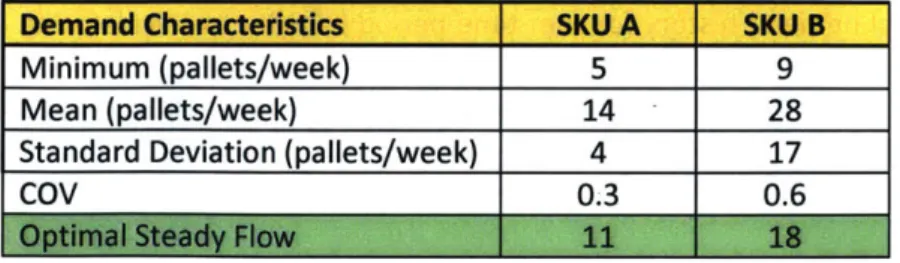
Results for selected eligible SKUs with different demand characteristics are discussed below. All numerical figures have been altered to mask real data. Table 4-1 presents the demand

characteristics of the selected SKUs.

Table 4-1 - Demand characteristics of selected SKUs

Demand Characteristics SKU A SKU B

Minimum (pallets/week) 5 9

Mean (pallets/week) 14 28

Standard Deviation (pallets/week) 4 17

COV 0.3 0.6

Optimal Steady Flow 11 18

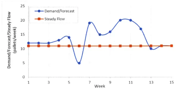
SKU A represents a typical product that has a non-zero demand throughout the demand

horizon. Its demand varies with a mean of 14 and standard deviation of 0.3, as noted in Table

4-1. Figure 4-1 illustrates the fluctuating demand and the corresponding optimal steady flow for this SKU.

25 -4- Demand/Forecast 20 -U-Steady Flow 151 10 5 1 3 5 7 9 11 13 Week

Figure 4-1 -Demand and Steady flow for SKU A

Figure 4-2 illustrates how the model determined the optimal steady flow. As can be seen, as the steady flow increases to up to 9 pallets a week, the transportation and cross-dock savings continue to rise without incurring noticeable excess inventory costs. However, as the steady flow is increased beyond 9 pallets per week, the excess inventory costs rise rapidly. The total savings are maximized at 11 pallets per week. The optimal steady flow determined for SKU A was in between the minimum pallets shipped and the mean pallets shipped over the model horizon. 0 U- M~-0 M

E

-0- Transportation Savings -- Cross-Dock Savings

-A- Inventory Cost -4-Total Savings

5 6 7 8 9 10 1 12 13 14 15

Steady Flow (# of pallets/week)

Figure 4-2 - Effect of change in steady flow on total costs for SKU A

This can be compared to SKU B, which is similar to SKU A in that it is shipped regularly with

non-zero demand over the full model horizon, but has a higher COV than SKU A, as shown in

Table 4-1. Figure 4-3 illustrates the fluctuating demand and the corresponding optimal steady

flow for this SKU.

80 70 .2 LL60 0 J. 30 m20 E a 10

0

Figure 4-3 - Demand and Steady Flow for high COV SKU B

Figure 4-4 illustrates how the model determined the optimal steady flow at 18 pallets per week, which, like SKU A, is between the minimum and mean of the demand.

-4- Transportation Savings -*-Cross-Dock Savings - I- Inventory Cost --- Total Savings

Mr 9

-7 12 17

Steady Flow (# of pallets/week)

Figure 4-4 - Effect of change in steady flow on total costs for SKU B

22 27 - - - - --- IF-

--Oj

The optimized steady flow for SKU A is closer to the mean than it is to the minimum of the

demand. In contrast, the optimized steady flow for SKU B is closer to the minimum than it is to the mean of the demand (Table 4-1). As any SKU's COV gets higher, the closer the steady flow will be to the minimum of the demand. This is because as the variation in demand

increases, having a higher steady flow increases the risk of bloating the inventory downstream.

As the percentage of weeks with demand decreases in the model horizon, the steady flow also gets closer and closer to the minimum. In other words, the more weeks that have zero demand for any given SKU the closer the steady flow will be to the minimum amount of

demand.

4.1.2. Effect of Parameters on Model Performance

The final output of this analytical model provides a list of recommended SKUs along with their optimal steady flow quantities. This output is influenced by the model's input parameters,

some of which should be tuned in order for the final output to be truly optimal. As mentioned in section 3.3, a definitive screening analysis was performed in order to visualize the effect of changing values on certain input parameters using JMP. This was done by running the model

and determining the optimal SKU mix and steady flow amount for each week over the course of 6 months. The steady flow amounts were then compared to actual demand history for that time period in order to calculate the actual total savings. The total savings and savings

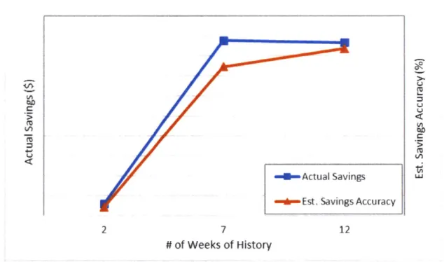
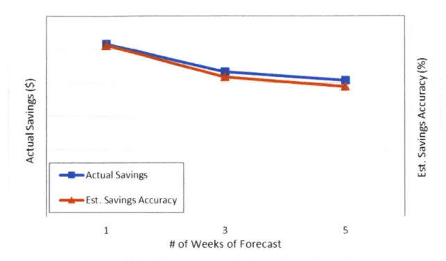
The inputs to the model horizon were selected for tuning as they directly affect the quantity and type of data being used in the model itself. History lengths of 12 weeks, 7 weeks, and 2 weeks were observed as well as forecast lengths of 1 week, 3 weeks, and 5 weeks. Based on the results of the screening, it is clear that using a higher length of history and a shorter length of forecast increases total actual savings and estimated savings accuracy (Figure 4-5 & Figure 4-6). The more history and less forecast data used in calculating the descriptive statistics during the SKU eligibility process, the better the model's performance. This was primarily because of the observed bias of the forecast in the given dataset.

-en-Actual Savi -mEst. Saving 2 7 ngs s Accuracy 'I M LA Vi 12 # of Weeks of History

Figure 4-5 - Effect of length of history on actual savings and estimated savings accuracy

4.' M

U

-

Actual Savings

MEst.

Savings Accuracy

1 3 5

# of Weeks of Forecast

Figure 4-6 - Effect of length of forecast on actual savings and estimated savings accuracy

The inputs to the eligibility criteria were also selected for tuning as they are the gate through

which all SKUs must pass in order to be considered for steady flow. Five COV values were

analyzed

0.4, 0.6, 0.8, 1.0, and 1.2. This range of values was representative of the majority

of SKUs on the given lane. As seen in Figure 4-7, a COV of 0.4 resulted in a 7% jump in

estimated savings accuracy. The remaining values yielded little change from one another in

terms of accuracy. The actual savings increased by 50% when going from a COV of 0.4 to 1.2.

This concurs with the fact that the overall number of SKUs becoming eligible also doubled.

M

---- Actual Savings

-- di-- Est. Savings Accuracy

0.4 0.6 0.8 1.0 1.2

Coefficient of Variation (COV)

Figure 4- 7 - Effect of change of threshold coefficient of variation of demand on actual savings and estimated

savings accuracy

Five values were also used to test percentage of weeks with demand - 50%, 60%, 70%, 80%, and 90%. There was no significant change in estimated savings accuracy between these values observed, but there was a 5% decrease in actual savings when going from 50% to 90% (Figure 4-8). This is due to the stricter requirement for SKUs, which constricted the amount of eligible SKUs by 10%.

C

.15

'U

Ln

-4b-Actual Savings - Est. Savings Accuracy

50 O 60% 70%

% Weeks with Demand

Figure 4-8 - Effect of change of threshold % of weeks with demand on actual savings and estimated savings accuracy

Three values were also used to test percentage of forecast weeks with nonzero forecast -40%, 60%, and 80%. There was no significant change in estimated savings accuracy between these values observed, but there was a 3% decrease in actual savings when going from 40% to 80% (Figure 4-9). This makes sense as the overall number of eligible SKUs decreased by 4%.

C

.5

40% 60%

% Forecast Weeks with Non-Zero Forecast

CD

.5

CU

80%

Figure 4-9 - Effect of change of threshold % forecast weeks with non-zero forecast on actual savings and estimated savings accuracy

The COV was observed to be the critical input parameter that influenced the actual savings and model accuracy the most. Either the actual savings or the model accuracy was maximized depending on which way the COV was being tuned. The other two parameters had minor effects, but were not nearly as impactful compared to the COV.

4.2. Assumptions and Limitations

The methodology described in Section 3.2 was developed as a framework for determining which SKUs could provide cost savings when converting some of the base demand into a steady flow. The model is intended to take into account the key costs and enable the study of the relationship between demand characteristics and the input parameters for SKUs on the steady flow. The

assumptions made in the model along with some additional opportunities for further research are described below.

4.2.1. Data Aggregation

As discussed in Section 3.2, this research uses demand data aggregated at a weekly level.

Thus, all calculations were done using a week as the unit of time. This approach enabled the analysis of a year's worth of data to build and refine the model without requiring advanced

data management packages. However, the methodology developed in this research applies to any given time unit for which relevant data is available. Estimation of cross-dock savings

and excess inventory costs may be more accurate if the calculations were based on a shorter time interval. Hence, it is recommended that future research be flexible in order to determine the best level of aggregation.

4.2.2. Vehicle Capacity Utilization

As discussed in Section 3.2.3, once the product flow between the plant and warehouse is

determined, the number of vehicles required needs to be calculated. The number of vehicles required for a given steady flow primarily depends on the achieved vehicle capacity

utilization.

As explained in Section 3.2.3, our approach takes into account target vehicle capacity utilization, albeit in a simplified manner. The optimization treats the individual SKUs in a binary fashion. Either a SKU is included in the final list or it is not. The reason for approaching

the optimization as a binary decision is because the total savings curve is non-linear. This is also done to keep the model simple enough to be able to study the impact of changes in

steady flow on cost savings. In practical implementation, it may be possible to find other combinations to maximize the vehicle capacity utilization. In addition, it is possible that the

overall vehicle capacity utilization of the whole lane is affected negatively due to some SKUs flowing on steady flow and others following the traditional process. This was not included in the scope of this study. In future studies, it is recommended that these two effects of vehicle capacity utilization be incorporated into the optimization to determine the steady flow.

4.2.3. Other Cost Considerations

The model developed in this research uses transportation savings, cross-dock productivity savings, and excess inventory as the primary cost considerations. Some additional cost

considerations, such as effect on safety stock requirements, replenishment frequency, planning process productivity, and environmental sustainability were not used directly in the

model calculations. These considerations are discussed briefly below. i. Safety Stock Requirements:

As noted in Section 3.2, the products on the steady flow skip the order-plan-ship process. For this reason, their effective lead-time from the plant to the warehouse decreases. Safety stock requirements at the warehouse depend on the lead-time; thus, a decrease

in lead-time will cause a reduction in safety stock requirements.

ii. Replenishment Frequency:

By definition, the products on the steady flow move from the plant to the warehouse consistently. In theory, a shipment reaches the warehouse every day of the week, and the

replenishment cycle time for steady flow products is minimized. The steady flow also decreases the risk of stock-outs, reduces the number of expedited shipments required, and increases the responsiveness of the supply chain.

iii. Planning Process Productivity:

Since the products on the steady flow skip the order-plan-ship process, only a weekly

effort is required to plan the shipment instead of the traditional daily exercise. This new process can contribute to lower time and effort required on behalf of the planning staff

after the initial determination of steady flow of containers/trucks is set. iv. Environmental Sustainability:

Taking into account vehicle capacity utilization as discussed in 4.2.2, steady flow has an

implication on the total number of vehicles that flow on the given lane. A lower number of vehicles contributes to lower fuel requirements and carbon emissions, and thus has a

positive effect on the carbon footprint of the organization. In the past decade, more and more organizations are measuring their carbon footprint and using it as a performance metric. Therefore, this might be a relevant cost to include in the steady flow determination.

These additional considerations have not been included in the current research. An extension of this research should include the above considerations for a more comprehensive cost

calculation.

4.2.4. Forecast Accuracy

As discussed in Section 3.2, the approach used in this research utilizes historical as well as forecast data to calculate the steady flow. Using the forecast data helps to incorporate effects

of seasonality, planned promotional activities, and discontinuation of products. However, as discussed in Section 3.3, it is critical to tune the input parameters to determine the

appropriate length of forecast to be used in the calculation.

As noted in Section 4.1.2, the given dataset yielded a negative correlation of accuracy of estimated savings and length of forecast used. This correlation can be attributed to the

observed bias of the forecast in the given dataset. For a given forecast length used, it is expected that as accuracy of forecast decreases, the estimated savings accuracy also decreases. Since this research was limited to testing the methodology using data for one lane only, the effect of increasing forecast accuracy on estimated savings accuracy could not be studied in detail. Future research applying this methodology to lanes with varying forecast

accuracy would be valuable in establishing and validating this relationship of forecast accuracy with the choice of parameters used.

4.2.5. Distribution Resource Planning (DRP)

Traditionally, the shipment frequency and volume for intra-company lanes, such as a plant-to-warehouse lane, is calculated by a Distribution Resource Planning (DRP) system. DRP is the

process by which multi-echelon distribution is carried out, taking into account safety stock requirements at various nodes. In most companies, this process is performed using an

automated system that analyzes future demand, starting inventory level, and safety stock requirements of the destination as well as planned deliveries. The objective of the DRP calculation is to maintain the destination safety stock levels and plan the product shipments

Having a steady flow of products from the plant to the warehouse would affect the DRP calculations described above. Since products on the steady flow skip the order-plan-ship

process, their lead-time is shortened. Most commonly used DRP systems currently do not allow for the use of multiple lead-times for a single lane. Thus, in this research, the steady

flow calculation is done outside of the DRP system. The calculation is then used as an input to DRP to determine the remaining flow of products between the plant and the warehouse. It is

recommended that in future studies, the DRP system be modified to include two different lead-times for the same lane. This modification would allow the steady flow calculations to

be integrated with the DRP calculations. Further research can be performed to evaluate the effect of steady flow changes on the lane's total flow.

4.2.6. Segmentation of Demand

In the current research methodology, as described in Section 3.2, all SKUs are subject to the same input parameters and eligibility criteria. Different categories of products flowing on the chosen lane may have varying forecast accuracy. For instance, class A SKUs, which have higher

demand and contribute more value to the company, may have more sophisticated demand planning methods, while slow moving, low margin products may have a less detailed forecasting process. Thus, segmenting SKUs according to their forecast accuracy may help in choosing appropriate parameters for each segment, improving steady flow optimization.

4.3. Implications

The analytical framework created for this thesis allows the company to have greater control over

their internal supply chain. The company can focus on maximizing potential savings and reducing internal costs while maintaining the same service levels to customers.

Many benefits and risks are involved when implementing a steady flow of products. This analytical framework is designed to maximize the benefits while minimizing the risks. Beyond providing an output of recommended SKUs and steady flow quantities, this framework allows for several other secondary benefits for the company that are not quantified in the model.

4.3.1. Bullwhip Dampening

One such benefit is the reduced variability that a company will have in upstream order

processes. By using downstream demand as a tool for proactive upstream planning, the company will experience a bullwhip dampening effect. Instead of becoming reactionary to the bulk ordering habits of downstream warehouses, plants can instead better match the

ongoing demand of the output at the warehouses.

This steady flow of products and reduced variability would potentially allow for reduced inventories and safety stock. The cost savings associated with this benefit are not quantified

in the model as this would be a business decision. However, the savings for this benefit could be significant.

4.3.2. Transportation Contract Innovation

Another secondary benefit that would be achieved by implementing a steady flow of products is stronger partnerships with transportation providers. The transportation savings calculated in the model is based on lower contracted prices per truck/container due to fixed volume

contracts. These contracts are mutually beneficial to the company as well as to the transportation providers. The company enjoys lower rates for the same service, and they also

enjoy a reduction in lead-time since the typical order-plan-ship process is eliminated. The transportation provider enjoys better asset planning as well as driver planning which helps

reduce uncertainty. Fixed volume contracts are also attractive to over-the-road transportation providers, as they provide more stable work schedules for employees, which reduces driver attrition rates. All of these benefits may allow for stronger strategic

partnerships and additional synergies.

4.3.3. Applicability

This analytical framework was created in the context of a fast moving consumer goods company, but this framework is applicable to any company in any industry. Any company that

moves high volumes - meaning several trucks/containers a day - of product on a single lane within its own network can use this model to take advantage of all of the benefits described above. The framework was built so that all of the parameters could be easily adjusted to align with any company's business processes as well as be tuned to the specific needs of any given

lane. In addition, the use of historical and forecast data over a moving model horizon enables the model to adapt and recommend the optimal steady flow for each time period.

5. Conclusion

Significant research has been done to study level production and its merits, but steady product flow between nodes of a supply chain had not been studied as much. The goal of this thesis was to develop

an analytical framework for determining the products that could flow on an intra-company lane regularly. This steady flow of products between supply chain nodes can lower transportation costs, increase cross-dock productivity, as well as dampen the bullwhip effect upstream in the supply chain. This research was done in the context of a plant-to-warehouse lane of a fast moving consumer goods

company.

The methodology developed in this research utilizes historical and forecast data to characterize the

demand. Descriptive statistics are used to determine whether a SKU is eligible for steady flow. Subsequently, transportation cost savings, cross-dock savings, and excess inventory considerations are used to optimize the quantity of each eligible SKU on steady flow. The model considers additional

business constraints of vehicle capacity utilization and then recommends a final list of SKUs and

quantities for the steady flow. This methodology was tested on a high volume plant-to-warehouse lane. Insights about the relationship between the variation in demand and steady flow were presented. As the coefficient of variation decreases, the optimal steady flow moves closer to the mean

of the non-zero historical demand and selected forecast over the model horizon.

Areas for future enhancements to this framework include optimal data aggregation, forecast accuracy implications, expansion of cost considerations, and implications on DRP. This research opens up the

possibility of realizing cost savings by decreasing transportation costs and improving warehouse productivity, paving the way for innovative contract types with transportation providers. This framework allows shippers to bridge the gap between steady flow theory and implementation.

References

Behdani, B., Fan, Y., Wiegmans, B., & Zuidwijk, R. (2016). Multimodal schedule design for synchromodal freight transport systems. European Journal of Transport & Infrastructure

Research, 16(3), 424.

Deif, A. M., & ElMaraghy, H. (2014). Cost performance dynamics in lean production leveling. Journal

of Manufacturing Systems, 33(4), 613-623. https://doi.org/10.1016/j.jmsy.2014.05.010

Garrido, R. A. (2007). Procurement of transportation services in spot markets under a double-auction scheme with elastic demand. Transportation Research Part B: Methodological,

41(9), 1067-1078. https://doi.org/10.1016/j.trb.2007.04.001

Kulwiec, R. (2004). Crossdocking as a Supply Chain Strategy. Retrieved December 4, 2016, from http://www.ame.org/sites/default/files/target_articles/04-20-3-Crossdocking.pdf Lindsey, C., & Mahmassani, H. S. (2016). Sourcing truckload capacity in the transportation spot

market: A framework for third party providers. Transportation Research Part A. https://doi.org/10.1016/j.tra.2016.10.001

Pfoser, S., Treiblmaier, H., & Schauer, 0. (2016). Critical Success Factors of Synchromodality: Results from a Case Study and Literature Review. Transportation Research Procedia, 14, 1463-1471. https://doi.org/10.1016/j.trpro.2016.05.220

Pirkul, H., & Jayaraman, V. (1996). Production, transportation, and distribution planning in a multi commodity tri-echelon system. Transportation Science, 30(4), 291-302.

Riessen, B., Negenborn, R. r., Dekker, R., Corman, F., VoR, S., & Negenborn, R. r. (2015). Synchromodal Container Transportation: An Overview of Current Topics and Research Opportunities. In F. Corman, S. VoR, & R. r. Negenborn (Eds.). Presented at the

Computational Logistics. 6th International Conference, ICCL 2015. Proceedings: LNCS 9335, Springer International Publishing. https://doi.org/10.1007/978-3-319-24264-4_27

Suh, E., essuh@snu.ac. k. (2015). Cross-docking assessment and optimization using multi-agent co-simulation: a case study. Flexible Services & Manufacturing Journal, 27(1), 115-133. https://doi.org/10.1007/s10696-014-9201-3

van Duin, J. H. R., Tavasszy, L. A., & Taniguchi, E. (2007). Real time simulation of auctioning and re-scheduling processes in hybrid freight markets. Transportation Research Part B:

Methodological, 41(9), 1050-1066. https://doi.org/10.1016/j.trb.2007.04.007

Zhelev, G. (2001). Flexibility in Transportation Procurement: A Real Options Approach, Masters Thesis, Massachusetts Institute of Technology.