Multicast tree structure and the power law

Multicast Tree Structure and the Power Law

Cedric Adjih & Philippe Jacquet Leonidas Georgiadis Wojciech Szpankowski¤

INRIA Dept. Electrical & Computer Eng. Dept. of Computer Science Rocquencourt Aristotle Univ. Thessaloniki Purdue University

78153 Le Chesnay Cedex Thessaloniki, 54006 W. Lafayette, IN 47907

France Greece U.S.A.

{adjih,jacquet}@inria.fr leonid@eng.auth.gr spa@cs.purdue.edu

Abstract

One of the main bene…ts of multicast communication is the overall reduction of network load. To quantify this reduction, when compared to traditional unicast, exper-imental studies by Chuang and Sirbu indicated the so called power law which asserts that the number of links L(m) in a multicast delivery tree connecting a source to m (distinct) sites satis…es L(m) ¼ cm0:8where c is a constant. In order to explain theoret-ically this behavior, Phillips, Shenker, and Tangmunarunkit examined approximately L(m) for a V -ary complete tree topology, and concluded that L(m) grows nearly lin-early with m, thus not obeying the power law. We …rst re-examine the analysis by Phillips et.al. and provide precise asymptotic expansion for L(m) that con…rms the nearly linear (with some wobbling) growth. Claiming that the essence of the problem lies in the modeling assumptions, we replace the V -ary complete tree topology by a V -ary self-similar tree with similarity factor 0 · µ < 1. In such a tree a node at level k is replicated CV(D¡k)µ _{times, where D is the depth of the tree and C is a constant.}

Under this assumption, we analyze again L(m) and prove that L(m) » cm1¡µ _where

c is an explicitly computable constant. Hence self-similar trees provide a plausible ex-planation of the multicast power law. Next, we examine more general conditions for general trees, under which the power law still holds. We also discuss some experimental results in real networks that rea¢rm the power law and show that in these networks the general conditions hold. In particular, our experiments show that for the tested networks µ ¼ 0:12.

1

Introduction

Multicast communication in the internet was proposed a decade ago in [1, 6] (cf. also [5]), and the experimental MBone network has been operational since 1992. In multicast communication senders transmit to logical address while receivers join a logical group. Mul-ticast routing ensures that only a single copy of a packet destined to multiple destinations traverses each link, so that the overall tra¢c load is reduced signi…cantly. Also, multicast alleviates the overhead on senders who can reach an entire group by the transmission of a single packet. The trade-o¤ is that multicast requires extra control and routing overhead at the routing nodes.

In this paper we concentrate on the quanti…cation of the main advantage of multicast routing. That is, we address the question of what is the expected tra¢c load reduction due to multicasting, when compared to unicast communication. Only recently some e¤orts

were undertaken to address this question. Motivated by the problem of pricing multicast communications, Chuang and Sirbu [4] performed experiments on a number of real and generated network topologies. They measured the average number of links L(m); in the multicast tree needed to reach m randomly selected routing nodes from a given source. L(m) represents the average cost of multicast tree per unit of bandwidth (it is assumed that all destinations require the same bandwidth). If unicast communication is employed, then the communication cost per unit of bandwidth is U m where U is the average number of links in a unicast path. The e¢ciency gain of multicast versus unicast is re‡ected in how far L(m) deviates from the (unicast) linear growth. Chuang and Sirbu [4], after extensive simulations, concluded experimentally that L(m) = £(m0:8). Moreover, they found that the constant in front of m0:8does not change signi…cantly with network size. This naturally raises the following questions. Is this behavior speci…c to the chosen topologies, or should be expected for other topologies as well? In the latter case, what is the main characteristic of the topology (or the generated multicast trees) that causes the appearance of the power law? This paper attempts to provide theoretical answers to these questions.

The most intriguing result, in the Chuang and Sirbu paper is reproduced here in Figure 1. The authors of 1 considered a multicast tree with N routing nodes. Multiple destination hosts may be connected to the network through each routing node (e.g., each routing node may have a number of dial-in ports, or may have a LAN connected to one of its ports). A source and a number n; of multicast destination hosts, is picked randomly. A multicast tree using shortest paths from the source to each of the destinations is constructed. We denote by L(n) the average number of links of the multicast trees created by the above procedure. Note that the number of destination hosts n can be either smaller or larger that the number of routing nodes N (throughout the paper we rather work with n rather than with distinct number of routing nodes m). Therefore, the ratio a = n=N can vary from zero to in…nity. Figure 1 shows the Chuang and Sirbu …ndings concerning the ratio of L(n) to the average cost of unicast communication. For n small relative to N , i.e., for a small, the power law L(n) ¼ n0:8 _{seems to be exhibited. Deviation from the power law and a phase transition}

appears around a = 1, and saturation occurs for a À 1. Our goal is to provide a theoretical explanation of the behavior observed in Figure 1, based on topological features of multicast trees that we introduce in the paper.

The …rst attempt to explain the power law of Chuang and Sirbu was undertaken by Phillips, Shenker and Tangmunarunkit in [14]. The authors on [14] considered several network topologies and provided approximate analysis of L(n) which indicated that L(n) grows linearly rather than according to the power law (cf. (17) and (18) of [14]). To make sure the approximation of [14] did not tilt …nal results, we provide precise analysis of the tree topology considered in [14], (cf. Theorem 1) which con…rms that their result indeed gives a good approximation for the leading term for L(n) when a is small. Interestingly enough, for small a we discover some small oscillations of the coe¢cient in front of n.

There are various ways to attempt to resolve this discrepancy between experimental and theoretical …ndings. In this work we demonstrate that the essence of the problem lies in the modeling assumptions about the structure of the underlying multicast tree. Indeed, our experimental results suggest that the actual geometry of the internet is such that multicast trees cannot be modeled as the regular trees proposed in [14] but rather a new model must be introduced. Speci…cally, we start with a full V ¡ary multicast tree, i.e., a tree for which all the nodes except the leaf nodes have outdegree V . Next, between two successive

1 10 100 1000 10000 10000 1

10 100

tree saturation re gion

Normalized T

ress Cost L(n)/U(n)

n^0.8

N = 100

n

Figure 1: This is Figure 7 from Chunag and Sirbu [4] showing the phase transition of the ratio of the number of links traverse in multicast and the average path length in unicast versus the number of destinations n.

branchings of a multicast we add several concatenated relay (otherwise called unary) nodes, i.e., nodes at which no branching occurs. The average number of these concatenated nodes decreases exponentially as the distance (in number of branchings) from the source increases. More precisely, a node in such a tree at level k is replicated V(D¡k)µ times, where D is the depth of three tree and 0 · µ · 1 is the self-similarity factor. A tree with such a property is shown in Figure 2. In fact, in our analysis we study trees of this structure which, for reasons that will become apparent in Section 2, we call self-similar. For self-similar trees we proceed to show that the ratio R(n) = L(n)=U (n) (of the number of links in a multicast tree to the average path length in unicast) exhibits the power law. More precisely, we show that for small a = n=N it holds R(n) » (c + Ã(n))n1¡µ where c is an explicitly computable constant and Ã(n) is an oscillating function of rather small amplitude for small values of V . (cf. Corollary 4(i)). Moreover, this constant is independent of the number of routing nodes N , which is in agreement with the observed results in [4].

Motivated by our experimental results, we concentrate on certain conditions that seem to be satis…ed by multicast trees on real networks. These conditions refer to the number of routing nodes on a multicast tree that can be reached by a node on that tree. It turns out that self-similar trees satisfy these conditions, and furthermore we show that these conditions are su¢cient for the appearance of the power law (albeit in a weaker form than in self-similar multicast trees).

The paper is organized as follows. In the next section we consider a complete V ¡ary tree network topology and provide a precise analysis of L(n) for regular and self-similar trees (cf. Section 2). In Section 3 we provide more general conditions that guarantee the appearance of the power law. We provide experimental results in Section 4. In particular, for our experiments we …nd that µexp¼ 0:12 which con…rms the power law £(n0:88). Finally,

the Appendix contains derivations of our theoretical results. In passing, we should mention that our …ndings have been established by analytical techniques of the precise analysis of algorithms such as Mellin transform and complex asymptotics (cf. [10, 15]). We give a brief survey of these methods since they may be useful for the study of other problems of similar

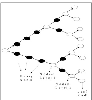
U n a r y N o d es N o d e at L e v e l 1 N o d e at L e v e l 2 L e a f N o de

Figure 2: A Self-Similar Tree with D = 3 and µ = 1.

nature.

2

Tree Topologies

In this section we present our results concerning regular and self-similar tree topologies. Derivations of the results are provided in the Appendix.

2.1

Regular Trees

As in [14], we consider a V ¡ary tree where the source is located at the root of the tree and all the potential destination hosts of the multicast tree are connected to the network through the leaf nodes of the tree. In Section 2.3 we consider the possibility that destination hosts may be connected to the network through other tree nodes, not just through the leaf nodes. We assume that behind each leaf node there may be multiple destination hosts. This is the case when, for example, each of the leaf nodes connects a LAN to the network. We may think of the V ¡ ary tree as the tree in a communication network G, composed of the shortest paths from the source to all the routing nodes of G. We refer to such a tree as the “global multicast tree” for the chosen source. When a number of the destination hosts in G needs to form a multicast group with the given source, they form a subtree of the global multicast tree. This subtree is used for multicast communication. Shortest path multicast trees were employed in the experiments in [4]. Multicast trees of this type are or can be used by several Internet multicast protocols such as DVMPRP [13], MOSPF [11], PIM-DM [7]. However, we should emphasize that the analysis that follows does not rely on the fact that the global multicast tree is a shortest path tree.

Let D be the depth of the tree, i.e., its longest (in terms of hops) path. We assume that the V ¡ ary tree is complete (all nodes but the leaves have outdegree V and all the leaves

are at depth D). If N is the number of leaf nodes then clearly

N = VD: (1)

Let the multicast group consist of n hosts and a = n

N > 0: (2)

Note that since more than one destination hosts may be behind each node, it is possible that a > 1. In order to explain the shape of Figure 1 we will deal with a in the region 0 · a < 1. However, the power law appears when a ¿ 1, which is the most interesting case from an analytical point of view, and the most likely one in practice. We assume that the probability of a host being connected to the network through a given leaf node is uniform and independent of the way the rest of the hosts are connected. In passing we point out, after the authors of [14], that if one insists on considering the number m of network nodes through which the destination hosts are connected to the network, then a good approximation is obtained by setting m = N (1¡e¡n=N) (cf. (1) of [14]). We underline again that throughout this paper we will work with the destination host multiply n rather than with m. Note that when a ¿ 1, then from the above approximation we obtain m ¼ n. As the power law is manifested when a ¿ 1, the results are qualitatively the same whether we work with n or m. We choose to work with n since the analysis is simpler in this case and, moreover, the method of choosing n destination hosts independently appears more natural.

Following Chuang and Sirbu [4], to quantify the reduction of tra¢c load in multicast over unicast, we shall analyze the average number of links L(n) in the multicast tree that connects n randomly selected hosts. If U denotes the average path between the source and a host in the unicast transmission, then the reduction ratio R(n) is de…ned as

R(n) = L(n)

U : (3)

Observe that for the complete V -ary tree we have U = D.

To estimate the average number of links in the multicast tree connecting n nodes, we observed that at level k of the tree, 1 · k · D, there are Vk _{links; the probability that a}

particular link is in the multicast tree after n destination hosts have been selected is 1 ¡ (1 ¡ 1=Vk)n:

Thus the average number of links in the multicast tree is L(n) = D=logXVN k=1 Vk ³ 1 ¡ ³ 1 ¡ V¡k ´n´ : (4)

Our goal is to estimate L(n) asymptotically as n ! 1 for …xed a (cf. Theorem 1), as well as for a ! 0, a ! 1 and a ! 1 (cf. Corollary 2).

Since V¡(D¡k) = aVk_{=n, in order to evaluate (4), it seems natural to replace 1 ¡ (1 ¡} V¡(D¡k))n _{by 1 ¡ e}¡aVk, take the upper sum index D = log_V N to be in…nity, and then sum up. However, this direct approach leads to incorrect results since the upper index D = log_{V N is at the cu¤-o¤ of a signi…cant contribution coming from (1 ¡ 1=V}k₎n_{and the}

in…nite series diverges. We need to be much more careful. In the Appendix we prove the following result.

Table 1: Comparison of the exact L(n) with the asymptotic expansion Lasym(n) obtained in Theorem 1 and the approximation LPST(n) proposed by Phillips, Shenker, and Tangmu-narunkit [14] for a = 0:5, that is, N = 2n.

N L(n) Lasym_{(n) L}PST_(n) 2 3.250 3.202 4.885 4 7.919 7.895 9.771 8 17.295 17.283 19.541 16 36.083 36.057 39.083 32 73.609 73.605 78.166 64 148.704 148.702 156.332 128 298.896 298.896 312.665 256 599.283 599.282 625.330 512 1200.056 1200.056 1250.650 1024 2401.602 2401.602 2501.320

Theorem 1 For …xed a, _{0 < a = n=N < 1, and large n (hence large N) the average} number of traversed links L(n) attains the following asymptotic expansion

L(n) = N µ V V ¡ 1¡ c1(a) ¶ ¡ V V ¡ 1 ¡ 1 2c2(a) + O µ 1 log n ¶ ; (5) where c1(a) = 1 X l=0 V¡lexp³_¡aVl´; (6) c2(a) = 1 X l=0 aVlexp³_¡aVl´: (7)

The quantities c1(a) and c2(a) converge quickly and hence (5) provides a convenient

way for the approximate computation of L(n). In order to verify the accuracy of the above asymptotic expansion (denoted Lasym(n) in Table 1) we compare it to the exact formula L(n) and the approximation LPST(n) proposed by the authors of [14]. From Table 1 one concludes that the asymptotic expansion presented in Theorem 1 is very good, even for small values of n.

From Theorem 1 one also must conclude that R(n) » ND(V =(V ¡ 1) ¡ c1(a)), which most

de…nitely does not exhibit the power law for general a. But, Figure 7 of [4] (cf. Figure 1) suggests that the power law appears only for small values of a, while for large values of a one should expect a saturation. To explain this situation, in the corollary below we analyze (5) for a ! 0, a ! 1 and a ! 1. This is equivalent to estimating asymptotically the constants c1(a) and c2(a) for these three regimes.

(i) For a ! 0 the quantity L(n) attains the following asymptotics L(n) = n µ D + 1 ln V ¡ ln n ln V + µ 1 2 ¡ ° ln V ¶ + Ã1(ln a) ¶ ¡ V V ¡ 1 ¡ 1 2 ln V + 1 2Ã2(ln a) + O µ 1 log n ¶ ; (8)

where ° = 0:571 : : : is the Euler constant, and Ã1(x), Ã2(x), are oscillating periodic

func-tions of small amplitude for small V that can be expressed as Ã1(x) = 1 X k=¡1 k6=0 ¡(¡1 ¡ 2¼ik= ln V ) ln V exp ³ 2¼ik x ln V ´ ; (9) Ã2(x) = 2¼i 1 X k=¡1 k6=0 k¡(¡2¼ik= ln V ) ln2V exp ³ 2¼ik x ln V ´ : (10) In fact, jÃ1(x)j < 0:0000001725; 0:00041227; 0:0085; 0:068; 0:153 for V = 2; 3; 5; 100; 1000, respectively.

(ii) For a ! 1 we have L(n) = N µ V V ¡ 1¡ C1¡ C2(a ¡ 1) + C3(a ¡ 1) 2 ¶ ¡ V V ¡ 1¡ C3 2 a + O µ 1 log n ¶ ; (11) where C1= 1 X l=0 V¡le¡Vl; C2 = 1 X l=0 e¡Vl; C3 = P₁ l=0Vle¡V l 2 :

(iii) For a ! 1 we arrive at L(n) = N µ V V ¡ 1 ¡ e ¡a ¶ ¡ V V ¡ 1¡ 1 2 ¡ ae¡a+ aV e¡aV¢+ O µ 1 log n ¶ : (12) We can now compare the theoretical results of Corollary 2 to the experimental results of Chuang and Sirbu presented in Figure 1. In particular, taking into account that ln N = D ln V we see from (8) that the ratio R(n) for a ! 0 can be approximated by

RD(n) ¼ n µ 1 +1 ¡ ° ln N + ln V 2 ln N ¡ ln n ln N + ln V ln NÃ1(ln a) ¶

which again most decidedly is not of the power law form. However, one can argue that for large a ! 1 and …xed N formulas (11) and (12) could explain respectively the transition and saturation region of Figure 1.

We note that the approximate analysis in [14] lead to the approximation L(n) ¼ n (D + 1= ln V ¡ ln n= ln V ) :

From (8) we see that the main term that the approximate analysis missed, is d = (:5 ¡ :5772= ln V ) plus the oscillating function Ã1(ln a) which for small to medium V is of small

amplitude. The term d is small, i.e., ¡0:33272 · d < :5. Moreover, we must note that the approximation is valid for a ¿ 1.

2.2

Self-Similar Trees

In view of the results in the previous section, we conclude that we cannot explain the multicast power law based on the adopted modeling assumptions. As discussed in the introduction, we shall argue that a possible explanation is the assumption regarding the structure of the global multicast tree. In this section we show that if the tree has a “self-similar” structure in the sense to be discussed below, then we indeed have the power law behavior for small a.

As in the previous subsection, consider a V ¡ary tree where all possible hosts are located at the leaves of the tree. However, we assume now that the link connecting a node at level k and a node at level k ¡ 1 consists of a concatenation of a random number of links. Let `k be the average number of these links. We postulate that `k is a fraction of `k¡1, that is,

for some A we have `1 = A and

`k= Á`k¡1; 0 · Á · 1:

Therefore, `k= Ák¡1A: Setting Á = V¡µ we …nd,

`k= V¡µ(k¡1)A = `DV(D¡k)µ; µ > 0:

In the rest of the paper, we assume for simplicity and without loss of generality that `D = 1.

The last equality suggests another interpretation of µ. Observe that there are K = VD¡k leaves hanging from a node at level k; thus we reproduce such a node Kµ times.

We call a tree with the above structure, a self-similar V ¡ary tree with similarity factor µ. Figure 2 shows a binary self-similar tree with similarity factor µ = 1 and depth D = 3. Note that when µ = 0, we have the regular V ¡ ary tree. In the following we assume that 0 · µ < 1.

We analyze now Lµ(n) and Rµ(n) for self-similar trees. In particular, as before, we

derive Lµ(n) = D X k=1 V(D¡k)µVk³_{1 ¡}³_{1 ¡ V}¡k´n´; and for the average path length in a unicast connection we …nd

Uµ= D X k=1 V(D¡k)µ = N µ ¡ 1 Vµ_{¡ 1}: (13)

In the Appendix we prove the following asymptotic expansions for Lµ(n).

Theorem 3 For …xed a,_{0 < a = n=N < 1, and large n the average number of links L}µ(n)

in the self-similar tree attains the following asymptotic expansion Lµ(n) = N Ã Vµ¹ Vµ¹_{¡ 1}¡ c1(a; µ) ! ¡ N µ_Vµ¹ Vµ¹_{¡ 1}¡ 1 2c2(a; µ) + O µ 1 log n ¶ ; (14) where µ_{= 1 ¡ µ and} c1(a; µ) = 1 X l=0 V¡¹µlexp³_¡aVl´; (15) c2(a; µ) = 1 X l=0 aV(1+µ)lexp³_¡aVl´: (16)

Corollary 4 Under the same conditions as in Theorem 3, we …nd: (i) For a ! 0 the quantity L(n) attains the following asymptotics

Lµ(n) = Nµ à nµ¹ µ ¡ (µ) ¹ µ ln V ¡ Ã3(ln a) ¶ ¡ V ¹ µ Vµ¹_{¡ 1}¡ 1 2 µ¡ (µ) nµ_{ln V} ¡ 1 nµÃ4(ln a) ! + O µ 1 log n ¶ ; (17) where ° = 0:571 : : : is the Euler constant, ¡(µ) is the Gamma function, Ã3(a) and Ã4(a)

are oscillating periodic functions of small amplitude for small V that can be expressed as Ã3(x) = 1 X k=¡1 k6=0 ¡(¡1 + µ ¡ 2¼ik= ln V ) ln V exp ³ 2¼ik x ln V ´ ; (18) Ã4(x) = 1 X k=¡1 k6=0 (µ ¡ i2¼k= ln V )¡(µ ¡ 2¼ik= ln V ) ln V exp ³ 2¼ik x ln V ´ : (19)

(ii) For a ! 1 we have L(n) = N Ã Vµ¹ Vµ¹_{¡ 1}¡ C1(µ) ¡ C2(µ) (a ¡ 1) + C3(µ) (a ¡ 1) 2 ! (20) ¡ N µ_Vµ¹ Vµ¹_{¡ 1}¡ C3(µ) 2 a + O µ 1 log n ¶ where C1(µ) = 1 X l=0 V¡µle¡Vl; C2(µ) = 1 X l=0 Vµle¡Vl; C3(µ) = P₁ l=0V(1+µ)le¡V l 2 :

(iii) For a ! 1 we arrive at Lµ(n) = N Ã Vµ¹ Vµ¹_{¡ 1}¡ e ¡a ! ¡ N µ_Vµ¹ Vµ¹_{¡ 1}¡ 1 2 ³ ae¡a+ aV1+µe¡aV´+ O µ 1 log n ¶ : (21) Now we are in a position to explain Figure 1 and to justify the power law of Chuang and Sirbu [4]. Observe that for small a Corollary 4(i) and (13) suggest the following ap-proximation. R(n; µ) = L(n; µ) Uµ ¼ n 1¡µ³ Vµ_{¡ 1}´ µ ¡ (µ) (1 ¡ µ) ln V ¡ Ã3(ln a) ¶ ¡V ¡ V 1¡µ V1¡µ_{¡ 1}: (22)

Thus, we obtain the power law with exponent of n equal to 1 ¡ µ. In addition, we observe that the constant that multiplies n1¡µ is independent of the tree size, which also agrees with the experimental results. We see from Corollary 4(iii) that for a ! 1 with N …xed the ratio L(n) tends to (N V1¡µ_{¡ N}µV1¡µ)=(V1¡µ_{¡1). Of course this is to be expected, since in this} case all nodes belong to the multicast tree and hence L(n) is equal to the number of links in the global multicast tree. Finally, around a = 1 we have a transitive behavior predicted by Corollary 4(ii). Therefore, Figure 1 is explained under the assumption of self-similar multicast trees.

2.3

Hosts Located at Non-relay Nodes

In the previous sections we assumed that destination hosts are located at the leaves of the global multicast tree. If destination hosts can also be located at any of the non-relay nodes of the global multicast tree, then in order to …nd the average cost of multicast we argue as in Section 2 and …nd Lµ(n) = D X k=1 µ V(D¡k)µVk µ 1 ¡ µ 1 ¡V D¡k+1_{¡ 1} VD+1_{¡ V} ¶n¶¶ = VDµV µ(D+1) ¡ Vµ Vµ_{¡ 1} ¡ V D D¡1_X k=0 V¡µk à 1 ¡a Vk+1¡1 V ¡1 n !n :

The term of Lµ(n) that needs to be analyzed asymptotically is

Lµ(n) = D¡1_X k=0 V¡µk à 1 ¡a Vk+1_¡1 V ¡1 n !n :

This term has the same form as the one analyzed before and hence its asymptotic expansion has also the same form. Hence, the results are qualitatively the same as in the case where destination hosts are located at nodes at the leaves of the tree.

3

Generalization

Motivated by experimental results, see Figure 3 of Section 4, we provide in this section general conditions on the global multicast tree, that give rise to the multicast power law.

For a node A on the global multicast tree, de…ne by r(A) the number of destination tree nodes that can be reached by A, using the multicast tree links (the tree links are considered unidirectional). For example, in the self-similar tree in Figure 2 if destination hosts are located at leaf nodes, then we have r(A) = 1 if A is a leaf node or if A is a relay node between levels 2 and 3. If A is located at level 1 or if A is a relay node between levels 0 and 1 we have r(A) = 4 = 23¡1_{. We call r(A) the “reachability degree of A”.}

Let Q(k) the number of nodes with reachability degree k. If destination nodes are at the leaves of the global multicast tree, it is easy to see that for the regular V -ary tree, we have Q(k) = VD_k¡1 _{if k = V}l_{, 0 · l · D, and Q(k) = 0 when k is not a power of V . Similarly,}

taking into account that there are Vµ(D¡l)_{¡ 1 relay nodes between levels l ¡ 1 and l we …nd} that for the self-similar V -ary tree we have Q(k) = k¡1+µVD, if k = Vl_{, 1 · l · D and} Q(k) = 0 when k is not a power of V .

Now, let us de…ne by F (k) the number of tree nodes with reachability degree at least k. That is, F (k) = N X l=k Q(k):

For a self-similar tree of depth D, we have for 1 · k · N, F (k) = D X l=dlogVke Q(k) = N D X l=dlogVke Vl(¡1+µ) = N VdlogVke(¡1+µ)1 ¡ V (D¡dlogVke+1)(¡1+µ) 1 ¡ V¡1+µ : Hence, N V¡1+µk¡1+µ_{· F (k) ·} N 1 ¡ V¡1+µk ¡1+µ_:

From the previous discussion we conclude that for self-similar trees, F (k) is decreasing according to k¡1+µ. The experimental results in Section 4 (see Figure 3) con…rm that this latter relation holds in real networks as well. Hence it seems natural to ask whether networks satisfying relations of this type give rise to the multicast power law. It turns out that indeed this is the case as shown in the next theorem.

Theorem 5 If for the global multicast tree and 0 < µ < 1 it holds for large N

aNk¡1+µ· F (k) · ANk¡1+µ (23)

then we have for n · N, aN AN ¡(µ)µn1¡µ¡1 + O¡_maxfn¡1_{; n=N g}¢¢_{· R(n)} · A_aN N ¡(µ)µn1¡µ¡1 + O¡_maxfn¡1_{; n=N g}¢¢: The proof of Theorem 5 is given in the appendix. We see that under the generalized assumptions of Theorem 5 the power law appears again, albeit in a weaker form than in self-similar trees. Note that if AN = AS(N ) and aN = aS(N ) (as is the case for self-similar

trees with S(N ) = N ) then the bounds on R(n) for small n=N become independent of N .

4

Experiments

We conducted a set of experiments on a real network in order to provide further evidence of the power law. We used data that was graciously made available by Bill Cheswick and Hal Burch on their site Internet Mapping Project [3]: They run frequent traceroute-style path probe on registered Internet networks: these probes give a good approximation of the paths used to route packets to many Internet networks, and all together give an approximation of the tree starting from one host in the Internet to all other networks. We will use this data to construct a tree topology and a multicast tree.

The above experimentally built tree was used to generate a multicast tree and compute R(n). Here is a brief description of our experiment:

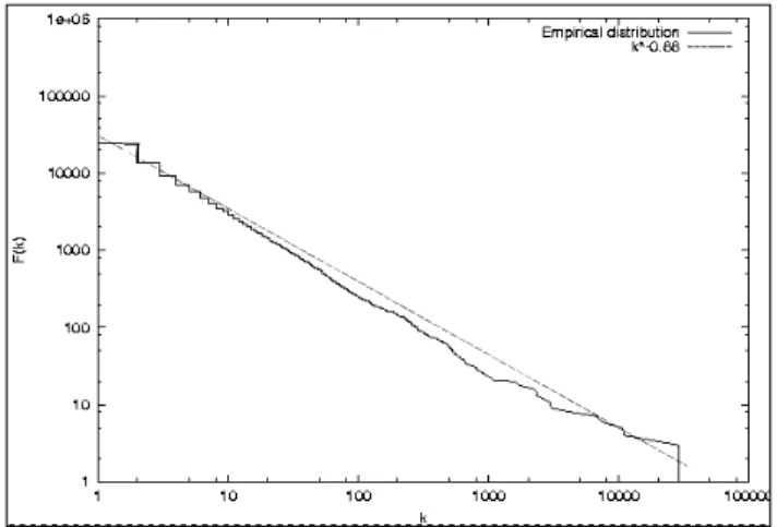
Figure 3: Log-log plots of F (k) versus k for the experimental tree.

² The total number of networks probed is 103625. ² The total number of successful probes is N = 28587. ² The destination hosts were all drawn randomly.

² After each draw, the size of the multicast tree is computed and updated along with the size of the unicast tree.

Note that not all probes are successful. This is due to the fact that probes rely on heuristics to guess what IP addresses are actually used in a given network. When an IP address is not correctly guessed, the probe isn’t taken into account. For each successful probe, a complete path to some network is found that lists all the intermediary routers. Using the set of all these probes, we build a tree. Given n, we pick a random number of n destination hosts and construct the multicast tree connecting the source to the routers at which the destination hosts are located. This multicast tree is a subset of the global multicast tree.

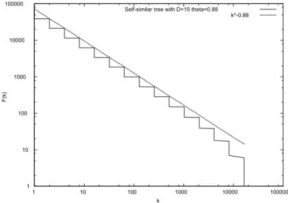
In Figure 3 we plot F (k), i.e., the number of routers in the global multicast tree that have reachability degree k, versus k. We see that F (k) is decreasing according to k¡:88. From the discussion in Section 3 we conclude that for this network, µ = 1 ¡ :88 = :12. For comparison in Figure 4 we plot F (k) versus k for a self similar tree with D = 15 and the same µ = :12.

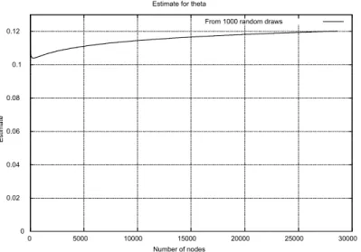
In Figure 5 we plotted R(n)=n versus n together with the curve f (n) = n¡0:12_{. In}

addition, in Figure 6 we plot µ versus n. The approximation seems to be very good. The previous experiments rea¢rm the power law for multicast trees as observed in [4].

1 10 100 1000 10000 100000 1 10 100 1000 10000 100000 F(k) k

Self-similar tree with D=15 theta=0.88 k^-0.88

Figure 4: F (k) versus k for the self-similar tree

0.20736 0.248832 0.298598 0.358318 0.429982 0.515978 0.619174 0.743008 0.89161 1 10 100 1000 10000 100000 Ratio Number of nodes Ratio Multicast_tree_size/Unicast_tree_size (log scales)

From 1000 random draws 1/n^0.12

0 0.02 0.04 0.06 0.08 0.1 0.12 0 5000 10000 15000 20000 25000 30000 Estimate Number of nodes Estimate for theta

From 1000 random draws

Figure 6: Experimental Curves for Estimating µ versus n.

5

Conclusions

In this paper we examined structural conditions on global multicast trees that give rise to the multicast power law. Regular V ¡ary trees do not exhibit the power law, while similar trees do. In fact, the power law rises under conditions weaker than tree self-similarity. Experimental work demonstrated that these latter conditions indeed hold for the tested networks.

The question whether multicast communication follows the power law arose from the attempt to price multicast communication in [4]. Power laws related to Internet topology parameters were studied in [8]. As indicated in the latter reference, power laws of this nature may be valuable for a¢rming how realistic simulated topologies are. This is an important issue that received a lot of attention [2], [16].

Our analysis provides a link between the structural properties of the global multicast tree and the generated multicast tree load. This leads to several new questions. Are the structural properties of the global multicast tree examined in this paper inherent to other networks as well? If so, what causes the appearance of this structure, and what is its implication in network performance, pricing, simulation etc? Is self-similarity an inherent multicast tree structure, or are networks with more general structure (e.g., appropriately behaving F (k)) the rule? Self-similarity implies an increased number of relay nodes (or in reality nodes with small outdegree) in the tree. Support for this property provide the experimental results in [8] and [12] where it is observed that the number of network nodes with small outdegree is a signi…cantly large proportion of the total number of nodes in the network (see Figure 6 in [8] and Figure 4 in [12]). However, further experimental work is needed in order to validate self-similarity or the more general conditions examined in this work. Of course, in real networks one does not expect simple V -ary trees or the appearance of self-similarity in the exact form presented here.

More generally, given the fact that several power laws related to various network para-meters have been observed experimentally, the question arises as to why these laws appear

and when one law implies the other. In this paper we touched one aspect of this big problem.

A

APPENDIX

In this appendix we establish our main theoretical results from Section 2. As observed before, our results for self-similar trees cover as the special case (µ = 0) the …nding for regular V -ary trees. Thus we concentrate here only on proving Theorem 3 and Corollary 4.

A.1

Proof of Theorem 3

We saw that the average cost of the multicast self-similar tree is

Lµ(n) = D

X

k=1

V(D¡k)µVk³_{1 ¡}³_{1 ¡ V}¡k´n´:

Observe that since D = log_V N and n = aN , for k = D the last term of the above sum is approximately equal to VD_{(1 ¡ e}¡a). This term is not small in general and thus we cannot extend the limit of the summation to in…nity without introducing signi…cant error. In order to provide an asymptotic analysis of Lµ(n), we de…ne ¹µ = 1 ¡ µ and proceed as follows:

Lµ(n) = D X k=1 V(D¡k)µVk³_{1 ¡}³_{1 ¡ V}¡k´n´= VD D¡1_X l=0 V¡¹µl µ 1 ¡ µ 1 ¡ V l VD ¶n¶ = VD Ã 1 ¡ V¡D¹µ 1 ¡ V¡¹µ ! ¡ VD D¡1_X l=0 V¡¹µl µ 1 ¡ V l VD ¶n = N Ã 1 ¡ N¡¹µ 1 ¡ V¡¹µ ! ¡ ¹Lµ(n); where ¹ Lµ(n) = N D¡1_X l=0 V¡¹µl µ 1 ¡aV l n ¶n : We shall use the following expansion for x · ln n

³ 1 ¡x n ´n = exp (¡x) Ã 1 ¡ x 2 2n + x nO Ã (ln n)3 n !! : (24) After setting An= $ ln¡ln n_a ¢ ln V % ; (hence ln n < eaVAn _{· e ln n) we obtain}

¹ Lµ(n) = N An X l=0 V¡¹µl µ 1 ¡aV l n ¶n + N D¡1_X l=An+1 V¡¹µl µ 1 ¡aV l n ¶n : (25)

We …rst look at the term An X l=0 V¡¹µl µ 1 ¡aV l n ¶n : For l · An we have aVl· ln n and hence from (24),

An X l=0 V¡¹µl µ 1 ¡aV l n ¶n = An X l=0 V¡¹µlexp³_¡aVl´ Ã 1 ¡a 2_V2l 2n + aVl n O Ã (ln n)3 n !! = An X l=0 V¡¹µlexp³_¡aVl´_¡ a 2N An X l=0 V(1+µ)lexp³_¡aVl´ + 1 Nµ¹O Ã (ln n)3+µ n1+µ ! + [[µ = 0]]ln N N O Ã (ln n)3 n ! ;

where [[µ = 0]] is equal to 1 when µ = 0 and zero otherwise. We now look separately at each of the above terms. We …nd

An X l=0 V¡¹µlexp³_¡aVl´= 1 X l=0 V¡¹µlexp³_¡aVl´_¡ 1 X l=An+1 V¡¹µlexp³_¡aVl´: (26) But 1 X l=An+1 V¡¹µlexp³_¡aVl´= 1 Nµ¹:O Ã 1 nµ_{(ln n)}µ¹ ! ; (27)

which …nally yields

An X l=0 V¡¹µl µ 1 ¡aV l n ¶n = c1(a; µ) ¡ 1 2Nc2(a; µ) + 1 Nµ¹O Ã 1 nµ_{(ln n)}µ¹ ! ; (28) where c1(a; µ) = 1 X l=0 V¡¹µlexp³_¡aVl´ (29) c2(a; µ) = 1 X l=0 aV(1+µ)lexp³_¡aVl´: (30)

To complete the proof of Theorem 3 we must estimate the term

D¡1_X l=An+1 V¡¹µl µ 1 ¡aV l n ¶n : But for l > An we …nd µ 1 ¡aV l n ¶n < µ 1 ¡ ln n_n ¶n = O(1=n); and hence D¡1_X l=An+1 V¡¹µl µ 1 ¡aV l n ¶n = V¡¹µAn_O µ 1 n ¶ =³ a ln n ´_µ¹ O µ 1 n ¶ = 1 Nµ¹O Ã 1 nµ_{(ln n)}µ¹ ! : (31) Combining our previous estimates we …nally prove Theorem 3.

A.2

Derivation of Corollary 4

We now prove Corollary 4, that is, we …nd asymptotic expansions of Lµ(n) for n: Observe

that we only need to analyze the quantities c1(a; µ) and c2(a; µ) de…ned in (15) and (16),

respectively. The regimes: (i) a ! 1 and (ii) a ! 1 are easy and are omitted due to lack of space.

Next we look at the regime a ! 0 which is the most interesting case, and the hardest. It turns out that this case can be handled by a special analytic tool, namely the Mellin transform. The Mellin transform found myriad of applications in the analysis of algorithms. The reader is referred to an excellent survey by Flajolet, Gourdon and Dumas [9] (cf. [10, 15]). For reader convenience, we collected the most important properties of the Mellin transform in Section A.4. In particular, the de…nition of Mellin transform is given in (34). Property (M2) de…nes the so called fundamental strip of the complex plane where the Mellin transform exists. The harmonic sum property (M3) and the mapping properties (M4) are crucial. We shall use them to derive asymptotics of c1(a; µ) and c2(a; µ) as a ! 0.

Let us …rst consider c1(a; µ) = P1l=0V¡¹µlexp

¡

¡aVl¢. Observe that by (M3) the sum in c1(a; µ) := c1(a) is a harmonic sum with ¸k= V¡k and g(x) = e¡x with ¹k= Vk. Thus

the Mellin transform c¤₁(s) with respect to a of c1(a) is by (M3) (and the well known fact

that the Mellin of e¡x _{is the Euler gamma function ¡(s) for <(s) > 0):} c¤₁(s) = ¡(s)

1 ¡ V¡(1+s¡µ):

We now use (M4) to …nd c1(a) as a ! 0, that is, we shall …nd the inverse to the Mellin

transform which according to (M1) is

c1(a) = 1 2¼i Z 1 2+i1 1 2¡i1 ¡(s) 1 ¡ V¡(1+s¡µ)x ¡s_{ds: (32)}

The goal is to apply the Cauchy residue theorem. But …rst we must consider a large rectangle left the the line, say from the line (1_{2 ¡ i1;}1_{2 + i1) to (¡M ¡ i1; ¡M + i1)} for some large M > 0. Due to the factor x¡s _{the left line contributes O(x}¡M_{) for any}

M > 0, which is negligible. The top and bottom lines of the big rectangle cancel out, thus the integral in (32) is equal to the residues inside the rectangle.

We now evaluate the residues. We note that the function c¤₁(s) has poles at sk =

¡1 + µ ¡ (2¼ik)= ln V ; k = §1; §2; :::. All these poles are single. The pole at 0 has residue c0;0 =

Vµ¹ Vµ¹_{¡ 1}:

The poles at sk, k 6= 1 have residues

c0;sk =

¡ (¡1 + µ ¡ 2¼ik= ln V )

ln V :

Using now the Reverse Mapping Theorem (M4) and the property ¡(¡1+µ) = ¡(µ)=(¡1+ µ), we see that for a ! 0 we have the expansion for any M > 0

c1(a; µ) = vµ¹ vµ¹_{¡ 1}¡ ¡ (µ) ¹ µ ln va ¹ µ + aµ¹Ã3(ln a) + O(aM); (33)

where Ã3(x) = 1 X k=¡1 k6=0 ¡(¡1 + µ ¡ 2¼ik= ln V ) ln V exp ³ 2¼ik x ln V ´ :

Now we consider c2(a; µ) = P1_l=0aV(1+µ)lexp¡¡aVl¢. It is again a harmonic sum,

hence by (M2) we …nd its Mellin transform to be c¤₂(a) = s¡ (s)

1 ¡ v¡(s¡µ):

But c¤

2(s) has a single poles at µ with residue

c0;0=

µ¡ (µ) ln v ;

and single poles at sk= µ ¡ (2¼ik)= ln V , k 6= 0 with residues

(µ ¡ i2¼k)¡(µ ¡ 2¼ik= ln V )

ln V :

Hence using again the Reverse Mapping Theorem (M4) we obtain c2(a; µ) = µ¡ (µ) ln V a ¡µ_{¡ a}¡µ_à 4(ln a) + O(aM) where Ã4(x) = 1 X k=¡1 k6=0 (µ ¡ 2i¼k= ln V )¡(µ ¡ 2¼ik= ln V ) ln V exp ³ 2¼ik x ln V ´ :

Combining everything we …nally prove Corollary 4.

A.3

Proof of Theorem 5

We …rst deal with L(n). Using Abel’s partial summation formula (cf. [15]) we observe that for two real-valued sequences vk and uk it holds

N X k=1 (uk¡ uk+1)vk = u1v1¡ uN +1vN + N X k=2 uk(vk¡ vk¡1):

Using this and taking into account that F (N + 1) = 0, we proceed as follows:

L(n) = N X k=1 Q(k) µ 1 ¡ µ 1 ¡_Nk ¶n¶ = N X k=1 (F (k) ¡ F (k + 1)) µ 1 ¡ µ 1 ¡_Nk ¶n¶ = N X k=2 F (k) µµ 1 ¡k ¡ 1 N ¶n ¡ µ 1 ¡ k N ¶n¶ + F (1) µ 1 ¡ µ 1 ¡ 1 N ¶n¶ = N X k=1 F (k) µµ 1 ¡k ¡ 1 N ¶n ¡ µ 1 ¡ k N ¶n¶ :

Now we deal with the upper bound. Using Taylor’s expansion we have µ 1 ¡k ¡ 1_N ¶n ¡ µ 1 ¡_Nk ¶n = n µ 1 ¡_Nk ¶_n¡1 1 N + O µ n2 N2 ¶ µ 1 ¡k ¡ 1_N ¶_n¡2 : Using this expansion and (23) we conclude

L(n) · ANNµ¡1n N X k=1 µ k N ¶_µ¡1µ 1 ¡ k N ¶_n¡1 1 N + ANNµ¡1n à _N X k=1 µ k N ¶µ¡1µ 1 ¡k ¡ 1_N ¶n¡2 ₁ N ! O³ n N ´ :

The function xµ¡1_{(1 ¡ x)}n¡1 is decreasing for 0 < x < 1: Therefore

N X k=1 µ k N ¶µ¡1µ 1 ¡_Nk ¶n¡1 ₁ N · Z 1 0 xµ¡1_{(1 ¡ x)}n¡1dx = ¯(µ; n) = ¡(µ)¡(n) ¡(n + µ); where ¯(µ; n) and ¡(x) are respectively the Beta and Gamma functions [15]. Also, we have

N X k=1 µ k N ¶µ¡1µ 1 ¡k ¡ 1_N ¶n¡2 ₁ N = N ¡µ₊ N X k=2 µ k N ¶µ¡1µ 1 ¡k ¡ 1_N ¶n¡2 ₁ N · N¡µ+ N X k=2 µ k ¡ 1 N ¶µ¡1µ 1 ¡ k ¡ 1_N ¶n¡2 ₁ N · N¡µ+ N X k=1 µ k N ¶µ¡1µ 1 ¡_Nk ¶n¡2 ₁ N · N¡µ+¡(µ)¡(n ¡ 1) ¡(n ¡ 1 + µ): Therefore, L(n) · ANNµ¡1n ¡(µ)¡(n) ¡(n + µ) + ANN µ¡1_n¡(µ)¡(n ¡ 1) ¡(n ¡ 1 + µ)O ³ n N ´ + ANNµ¡1nN¡µO ³ n N ´ : Using now the approximation [15],

¡(n) ¡(n + µ) = n ¡µ¡_{1 + O(n}¡1₎¢_; we have L(n) = ANNµ¡1n1¡µ¡(µ) ¡ 1 + O(n¡1)¢ + ANNµ¡1n (n ¡ 1)¡µ¡(µ) ³ 1 + O((n ¡ 1)¡1) ´ O³ n N ´ + ANNµ¡1nN¡µO ³ n N ´ = ANNµ¡1n1¡µ¡(µ) µ³ 1 + O(n¡1) + O³ n N ´´ + 1 ¡(µ)O µ³_n N ´1+µ¶¶ = ANNµ¡1n1¡µ¡(µ) ³ 1 + O(n¡1) + O³ n N ´´ ;

where in the last equality we used the fact that n < N . It remains to compute U (n). Arguing as above we obtain

U (n) = N X k=1 k NQ(k) = N X k=1 k N (F (k) ¡ F (k + 1)) = N X k=1 1 NF (k) ¸ aNNµ¡1 µZ 1 0 xµ¡1dx + O µ 1 N ¶¶ = aNNµ¡1µ¡1 µ 1 + O µ 1 N ¶¶ : The lower bound is derived in a similar fashion.

A.4

Main Properties of Mellin Transform

For the reader convenience, we collected here the main properties of the Mellin transform. For details and proofs see [9, 15].

(M1)Direct and Inverse Mellin Transforms. Let c belong to the fundamental strip de…ned below. Then

f¤_{(s) := M(f(x); s) =} Z ₁ 0 f (x)xs¡1dx ₍₎ f (x) = 1 2¼i Z _c+i1 c¡i1 f¤(s)x¡sds: (34) (M2) Fundamental Strip. The Mellin transform of f (x) exists in the fundamental strip <(s) 2 (¡®; ¡¯), where

f (x) = O(x®) _{(x ! 0);} f (x) = O(x¯) _{(x ! 1)} for ¯ < ®.

(M3)_{Harmonic Sum Property. By linearity and the scale rule M(f(ax); s) = a}¡s_{M(f(x); s),} f (x) =X k¸0 ¸kg(¹kx) () f¤(s) = g¤(s) X k¸0 ¸k¹¡_ks: (35)

(M4)Mapping Properties (Asymptotic expansion of f (x) and singularities of f¤_(s)).

f (x) = X (»;k)2A c»; kx»(log x)k+ O(xM) () f¤(s) ³ X (»;k)2A c»; k (¡1) k_k! (s + »)k_{+ 1}: (36)

— (i) Direct Mapping. Assume that f (x) admits as x ! 0+_{the asymptotic expansion (36)}

for some ¡M < ¡® and k > 0. Then for <(s) 2 (¡M; ¡¯), the transform f¤(s) satis…es the singular expansion (36)

— (ii) Reverse Mapping. Assume that f¤_{(s) = O(jsj}¡r_{) with r > 1, as jsj ! 1 and that}

f¤_{(s) admits the singular expansion (36) for <(s) 2 (¡M; ¡¯). Then f(x) satis…es the} asymptotic expansion (36) at x = 0+.

References

[1] S. Casner and S. Deering, “First IETF internet audiocast,” ACM Computer Communi-cations, 92-97, 1992.

[2] K. Calvert, M. Doar, and E. Zegura, “Modeling InternetTopology,” IEEE Commun. Magazine, 35, 160-163, 1997.

[3] B. Cheswick and Hal Burch, Internet Mapping Project, http://www.cs.bell-labs.com/who/ches/map/index.html.

[4] J. Chuang and M. Sirbu, “Pricing Multicast Communications: A Cost-based Approach,” Proceedings of the INET’98, 1998.

[5] S. Deering, “Multicast Routing in Inetrnetworks and Extended LANs,” Computer Com-munication Review, 18, 1998.

[6] S. Deering, and D. Cheriton, “Multicast Routing in Datagram Internetworks and Ex-tended LANs,” ACM. Trans. Computer Systems, 8, 85-110, 1990.

[7] D. Estrin, D. Farinacci, V. Jacobson, C. Liu, L. Wei, P. Sharma and A. Helmy, “Protocol Independent Multipast (PIM) sparse mode/dense mode,” Internet Draft, 1996.

[8] M. Faloutsos, P. Faloutsos, and C. Faloutsos, “On the Power-Law Relationship of the Internet Topology,” ACM SIGCOMM, Cambridge, 1999.

[9] P. Flajolet, X. Gourdon, and P. Dumas, “Mellin Transforms and Asymptotics: Harmonic sums,” Theoretical Computer Science, 144, 3–58, 1995.

[10] D. E. Knuth, The Art of Computer Programming. Sorting and Searching, Vol. 3, Second Edition, Addison-Wesley, Reading, MA, 1998.

[11] J. Moy, “Multicast Extensions to OSPF,” Internet Draft, 1998.

[12] J. Pansiot and D. Grad, “On Routes and Multicast Trees in the Internet,” ACM Computer Communication Review, 28, 41-50, 1998.

[13] T. Pusateri, “Distance Vector Routing Protocol,” Internet draft, draft-ietf-idmr-dvmrp-v3-07, 1998.

[14] G. Phillips, S. Shenker, H. Tangmunarunkit, “Scaling of Multicast Trees: Comments on the Chuang-Sirbu scaling Law,” SIGCOMM, Cambridge, 1999.

[15] W. Szpankowski, Average Case Analysis of Algorithms in Sequences, John Wiley & Sons, New York, 2001.

[16] E. W. Zegura, K. L. Calvert, and M. J. Donahoo, “A Quantitative Comparison of Graph-based Models for Internet Topology,” IEEE/ACM Transactions on Networking, 5, 1997.