Autonomous thruster failure recovery on underactuated spacecraft using model predictive control

Autonomous thruster failure recovery on underactuated

spacecraft using model predictive control

The MIT Faculty has made this article openly available.

Please share

how this access benefits you. Your story matters.

Citation

Pong, Christopher M., Alvar Saenz-Otero and David W. Miller.

"Autonomous thruster failure recovery on underactuated

spacecraft using model predictive control." In Guidance and

Control 2011: Proceedings of the 34th Annual AAS Rocky Mountain

Section Guidance and Control Conference, February 4-9, 2011,

Breckenridge, Colorado, Univelt, Inc. pp. 107-126. (Advances in the

astronautical sciences; v. 141)

As Published

http://www.univelt.com/linkedfiles/v141%20Contents.pdf

Publisher

Univelt, Inc.

Version

Author's final manuscript

Citable link

http://hdl.handle.net/1721.1/81885

Terms of Use

Creative Commons Attribution-Noncommercial-Share Alike 3.0

AUTONOMOUS THRUSTER FAILURE RECOVERY

ON UNDERACTUATED SPACECRAFT

USING MODEL PREDICTIVE CONTROL

Christopher M. Pong,

Alvar Saenz-Otero,

and David W. Miller

Thruster failures historically account for a large percentage of failures that have occurred on orbit. These failures are typically handled through redundancy, however, with the push to using smaller, less expensive satellites in clusters or formations there is a need to perform thruster failure recovery without additional hardware. This means that a thruster failure may cause the spacecraft to become underactuated, requiring more advanced control techniques. A model of a thrus-ter-controlled spacecraft is developed and analyzed with a nonlinear controlla-bility test, highlighting several challenges including coupling, nonlinearities, se-vere control input saturation, and nonholonomicity. Model Predictive Control (MPC) is proposed as a control technique to solve these challenges. However, the real-time, online implementation of MPC brings about many issues. A me-thod of performing MPC online is described, implemented and tested in simula-tion as well as in hardware on the Synchronized Posisimula-tion-Hold, Engage, Reo-rient Experimental Satellites (SPHERES) testbed at the Massachusetts Institute of Technology (MIT) and on the International Space Station (ISS). These results show that MPC provided improved performance over a simple path planning technique.

INTRODUCTION

Failure detection, isolation, and recovery is an integral part of any robust space-based system. If a satellite fails on orbit, currently there is little to no chance of being able to send an agent to that satellite and provide on-orbit servicing. Thus, it is paramount for a satellite to be able to tell if something is wrong (failure detection), determine what subsystem or component has failed (isola-tion), and appropriately change the system to handle this failure (recovery).

An extensive review has been performed of failures that have occurred on 129 military and commercial spacecraft from 1980 to 2005.1 It was determined that thruster failures account for 24% of all the attitude and orbit control subsystem failures. Because thruster failures are one of the more likely failures to occur on a spacecraft, many have developed ways to mitigate the effect of these failures. One of the obvious methods of handling these failures is through the use of

*

Graduate Research Assistant, Space Systems Laboratory, Department of Aeronautics and Astronautics, Massachu-setts Institute of Technology, 77 MassachuMassachu-setts Avenue, Cambridge, MA 02139.

†

Research Scientist, Space Systems Laboratory, Department of Aeronautics and Astronautics, Massachusetts Institute of Technology.

‡

Professor, Department of Aeronautics and Astronautics, Director, Space Systems Laboratory, Massachusetts Institute of Technology.

tional hardware. Sensors can be embedded in the thruster itself for thruster failure detection and additional redundant thrusters can be used to replace the failed thrusters. Additional hardware, however, impacts the cost, mass, volume, and power budgets of the spacecraft program.

For large, monolithic spacecraft with a cost budget on the order of billions of dollars, redun-dancy may well be justified. However, there is a move toward launching smaller, less expensive spacecraft. Examples include satellites developed for the Evolved Expendable Launch Vehicle (EELV) Secondary Payload Adapter (ESPA) ring and satellites adhering to the CubeSat standard. These satellites can be launched for a small fraction of the cost of a dedicated launch vehicle, dramatically driving down costs. There is also a push to replace the functionality of a monolithic spacecraft with multiple spacecraft (e.g., DARPA's System F6 Program). Including redundancy for each spacecraft to handle failures on top of this may be too costly to justify the benefits. With the prospect of smaller, less expensive spacecraft and having multiple spacecraft in a cluster or formation, methods of performing thruster failure recovery without the use of hardware redun-dancy has become a vital topic of research.

Overview of the SPHERES Testbed

To aid in the development and maturation of esti-mation and control algorithms for proximity opera-tions such as formation flight, inspection, servicing, assembly, the Massachusetts Institute of Technology (MIT) Space Systems Laboratory (SSL) has devel-oped the Synchronized Position Hold, Engage, Reo-rient, Experimental Satellites (SPHERES) testbed. This testbed consists of six nanosatellites: three at the MIT SSL and three on board the International Space Station (ISS). The three satellites on the ISS can be seen flying in formation in Figure 1. These satellites will serve as a representative spacecraft on which to

test the developed thruster failure recovery algorithm. Figure 1. SPHERES Satellites on the ISS. The SPHERES satellites contain all the necessary subsystem functionality of a typical satel-lite: avionics, communication, metrology, power, propulsion. Additional information on the SPHERES testbed can be found in References 2 and 3.

Testing in the space environment is typically a high-risk and costly endeavor where any ano-maly or failure can easily result in the loss of a mission. The SPHERES testbed provides re-searchers with the ability to push the limits of new algorithms by performing testing in a low-risk, representative environment. Three different development environments are used: the six-degree-of-freedom (6DOF) MATLAB simulation, the three-degree-six-degree-of-freedom (3DOF) ground testbed, and the 6DOF ISS testbed. These environments allow algorithms to be iteratively matured to higher levels of technology readiness.

SPACECRAFT MODEL

Before developing a control system that is able to handle thruster failures, a dynamic model of the spacecraft must first be developed and analyzed. First, a brief review of the equations of mo-tion of a thruster-controlled spacecraft is given, then the controllability of a SPHERES satellite is analyzed, and finally the challenges associated with controlling this system are elucidated.

Equations of Motion of a Thruster-Controlled Spacecraft

Thrusters are modeled as a body-fixed force that is applied to a set location on the spacecraft. The lever arms and thrust directions of all m thrusters can be arranged in matrices of size 3×m. The thruster lever arms are given by





where li represents the vector describing the lever arm of the i th

thruster in the body frame. The thrust directions are given by





where di represents the vector describing the direction of the i th

thruster in the body frame. The force provided by each thruster is given by a vector, u. It is important to note that these thruster forces are unilateral, meaning that they cannot produce negative thrust. A spacecraft is fully ac-tuated if a linear combination of these thruster forces can produce any arbitrary force and torque. If the spacecraft has more than enough thrusters, it is overactuated. On the other hand, if the spacecraft does not have enough thrusters (i.e., it cannot produce any arbitrary force and torque), it is underactuated. If a spacecraft is fully actuated, and a thruster fails off, the spacecraft becomes underactuated. Therefore, the reconfigurable control of an underactuated spacecraft is the same problem as recovering from a thruster failure.

These thruster control inputs drive both the translational and attitude dynamics. The position,

r, and velocity, v, of the spacecraft are described by the following kinematic and kinetic

equa-tions v r  (6)

 

where m is the spacecraft mass* and ΘT is the direction cosine matrix (DCM) that transforms the thruster body forces, Du, into the inertial frame (the same frame as position and velocity). This DCM is a function of the current spacecraft attitude, which is represented as a unit quaternion. This quaternion represents the rotation from the inertial frame to the body frame and is defined as









where a is the normalized axis of rotation and θ is the angle of rotation. With this definition of the attitude quaternion, the DCM is given by4

 





where the superscript × denotes the 3×3 skew-symmetric cross-product matrix associated with the 3×1 column vector. In general,

                           0 0 0 1 2 1 3 2 3 3 2 1 a a a a a a a a a a a . (10)

The equations of motion for the spacecraft attitude, q, and the angular rate, ω, can now be stated as

 





 









Equations (6), (7), (11), and (12) form the complete dynamics of a thruster-controlled spacecraft. The main assumptions of these equations are that the origin of the body is at the center of mass of the spacecraft, and that the spacecraft can be treated as a rigid body (no flexibility or slosh in the spacecraft).

Controllability

Now that the model for a thruster-controlled spacecraft has been developed, it is useful to de-rive the controllability of this system, which will give valuable insight into its complex nature. A system is controllable if for all states xi and xf there exists a feasible control input trajectory, u(t),

defined on the interval [0, T] such that the solution to the initial value problem x˙ = f(x,u) with

x(0) = xi has the solution x(T) = xf.

Despite its fundamental role in control theory, a completely general set of conditions for con-trollability of nonlinear systems does not currently exist.5 While there exist simple methods for determining controllability of linear, time-invariant (LTI) systems, it has been shown that these techniques, even when modified to handle the unilateral control inputs, does not provide complete controllability results for this system. This is because linearization ―freezes‖ the locations and directions of the thrusters and makes the controllability results only valid for a single attitude.6 More advanced controllability tests are necessary to gain further insight into this system.

Nonlinear controllability is considerably more complex than LTI controllability. The most de-veloped concept of controllability of nonlinear systems is restricted to systems that can be ex-pressed in control-affine form,

 

_

 





u

x

g

x

f

x

where x is the state, f is the drift vector field, ui is the i th

control input, and gi is the i th

control vec-tor field. In this formulation, it can easily be seen that the dynamics of the system are a linear combination of the drift vector field and control vector fields. Controllability can be viewed in terms of adjusting the coefficients, ui, to steer the system from one state to another.

An interesting property of these vector fields, arising from the nonlinear nature of the system, is that combinations of multiple vector fields can produce motion in directions of the state space that is not possible with a single control input. The flow along a vector field g from state x0 for

time t, φt g

(x0), is defined as the solution to the differential equation x˙ = g(x) with initial condition

x0. It can be shown 7

that the composition of flows along two vector fields, g1 and g2 for an

infini-tesimally small amount of time, ε,

 







 









 

 

 

 

4









O



























g

x

x

g

x

g

x

g

x

x

where O(ε3) denotes terms on the order of ε3 or higher. This result shows that the flow along these vector fields produces a net non-zero motion on the order of ε2, ignoring the higher-order terms. It is important to note that in this formulation, this net non-zero motion is valid only for states in the neighborhood of the initial state, x0. Therefore, this concept will be used to define small-time

* local controllability. This net non-zero motion can be captured in the definition of the Lie bracket

operation as†





 

 

The idea that Lie brackets can produce a non-zero vector field is connected with the idea of nonholonomicity. When a system contains nonintegrable constraints‡ it is considered nonholo-nomic. Since it is often difficult to directly determine whether a constraint is truly nonintegrable versus one's lack of ability to determine how to integrate it, one can employ the Frobenius theo-rem to determine whether a system is nonholonomic or holonomic. The Frobenius theotheo-rem states that a system is holonomic or integrable if and only if all Lie brackets are in the span of the origi-nal system vector fields.8 Inversely, a system is nonholonomic if and only if there are Lie brackets that are not spanned by the original system vector fields. Knowing whether or not a system is nonholonomic is important when considering the control system design.

Since the Lie bracket produces a new vector field, further vector fields can be defined recur-sively (e.g., g3 = [g1,[g2, g1]]). The degree of a vector field, δ(·), is the number of times the

origi-nal system vector fields appear in the Lie bracket operation (e.g., δ([g1,[g2, g1]]) = 3). The degree

with respect to a vector field, δgi(·), is the number of times gi appears in the Lie bracket operation

*

The qualifier ―small-time‖ indicates that it holds for any time greater than zero.

†

This definition of the Lie bracket operation is a specific definition for defining small-time local controllability. The Lie bracket operation can be defined in any way such that the following three properties hold: bilinearity, skew symme-try, and Jacobi identity.

‡

(e.g., δg1([g1,[g2, g1]]) = 2). Intuitively, the degree of a vector field is equivalent to a measure of

―speed‖ of the vector field. A higher degree corresponds to a slower motion.

It is also necessary to define ―good‖ and ―bad‖ Lie bracket terms. One minor detail that was excluded from the flow definition of a Lie bracket is that vector fields such as the drift vector field can only be followed in a single direction. For the example of the drift vector field, flow in the opposite direction can only be possible if time were reversed. Lie brackets that exhibit this asymmetry are therefore called ―bad.‖ A Lie bracket, φ, is bad if δf(φ) is odd and δgi(φ) is even

for all i = 1…m. The exact reasoning behind this definition of a bad Lie bracket is beyond the scope of this paper. The intuitive reasoning is that Lie brackets that meet these conditions have motions that contain only even exponents of the control inputs, ui, and can therefore only be

fol-lowed in a single direction.9 Another article gives an example where brackets that are seemingly bad (e.g., ones that have the drift vector field in them) can have their flows rearranged such that they are not bad.10 A Lie bracket that is not bad is called ―good.‖ It will be necessary, for control-lability, to have these bad Lie brackets be ―neutralized‖ by good brackets. A bad Lie bracket can be neutralized if it can be written as a linear combination of good Lie brackets of lower degree. Intuitively, this means that the illegal motion of a bad Lie bracket can be counteracted by the fast-er, legal motions of a good Lie bracket.

With the definition of the Lie bracket, the Lie algebra of the system vector fields, L({f, g1, …,

gm}) can now be defined. The Lie algebra includes all the system vector fields as well as all

vec-tor fields that can be produced by a finite number of nested Lie bracket operations.8 This vector space can be determined by finding an independent basis of vector fields which spans this vector space. Since finding this basis can be a tedious task, there is an approach that uses the Philip Hall basis to help prune the search space of possible nested Lie bracket operations.8

Now that all of the necessary tools for determining controllability have been developed, the conditions for small-time local controllability (STLC) can be stated. The control-affine system given by Equation (14) is STLC from x0 if:

1. The drift velocity field is zero at x0: f(x0) = 0.

2. The Lie Algebra Rank Condition is satisfied by good Lie bracket terms up to degree i: dim(L{f,g1, …, gm}) = span({φ1, …, φn | φ1, …, φn are good}) = n.

3. All bad Lie brackets of degree j ≤ i are neutralized. 4. Inputs are symmetric.

These are the sufficient conditions for STLC given in Reference 11 and summarized in Refer-ence 9. The first condition arises since the drift vector field is a bad Lie bracket. Since it cannot be neutralized by good Lie brackets since it is already of the lowest possible degree, it must be equal to zero. The second and third conditions ensures that the motion produced by all possible combinations of the vector fields spans the full n-dimensional space, while all bad Lie brackets that are encountered can be neutralized. The final condition ensures that the inputs are symmetric, meaning the control vector fields can be followed in both directions. While this is a problem with unilateral control inputs, the conditions for STLC have been generalized, to an extent, for unila-teral control inputs.10 These slightly generalized conditions will not be presented since the two approaches are equivalent in the case when thrusters are paired.* This highlights an important li-mitation of this analysis; when a single thruster has failed, its corresponding opposing thruster

*

must also be removed from the controllability analysis for this analysis to be valid. This is neces-sary since if a thruster fires without some set of thrusters that can immediately counteract it, this thruster firing necessarily produces a global change in state.

The STLC property is important for a few reasons. First, a system that is STLC implies that it is controllable under a few mild conditions.9 Second, it means that the system can follow a curve arbitrarily close as long as it hovers around zero-velocity states. This is a useful property for a system where obstacles need to be avoided since the necessary motion to avoid an obstacle can be acheived through a ―wiggling‖ motion. In contrast, a system that is controllable but not STLC may need to go through large state changes to achieve a desired state and can therefore not follow any arbitrary trajectory.

With the sufficient conditions above, the thruster-controlled spacecraft was tested to see if it is STLC. It turns out that the representative SPHERES satellite is STLC with all twelve thrusters operational, however does not pass the conditions for a single thruster failure. This is because the system has bad Lie brackets of degree three that cannot be neutralized.6 These results extend con-trollability results presented in Reference 12, which only considered a rigid body constrained to a plane. The fact that the spacecraft is not STLC, means that to steer the spacecraft to a particular position and attitude, global state changes must occur. Feasible trajectory design, especially with obstacles, becomes nontrivial.

It is important to note here that the STLC conditions presented are only sufficient conditions. Therefore, even if the conditions are not met, the system may still be STLC. This has been shown through counterexample. For example, Reference 13 showed that a system that does not meet the conditions for small-time local configuration controllability (STLCC), a concept very closely re-lated to STLC, can actually be transformed into a system that does meet the STLCC conditions. While it is possible that a transformation can be found that makes the presented system STLC even in the event of thruster failures, determining if such a transformation exists is beyond the scope of this paper. Therefore, it has not been proven that an underactuated spacecraft is not STLC. Rather, it can be said that the underactued spacecraft model presented (excluding any transformations) is not STLC given the set of sufficient conditions used.

Another conclusion that can be drawn from this analysis is that the spacecraft becomes second-order nonholonomic in the event of any thruster failure. This arises from the fact that when a thruster fails, the spacecraft becomes underactuated, causing a nonintegrable constraint on acceleration. Knowing that the system falls under the class of nonholonomic systems is useful to know when designing the control system.

Control System Design Challenges

Now that the spacecraft model has been developed and analyzed with nonlinear controllability techniques, the specific challenges with developing a control system for this spacecraft can be discussed. The main challenges are coupling of the translational and attitude dynamics, multiplic-ative nonlinearities, control input saturation, and nonholonomicity.

Coupling. In the formulation of the system dynamics, the control input, u, enters the system

through both the translational and attitude dynamics. A very common method of handling this issue is to decouple position and attitude by treating the control inputs as generalized forces and torques instead of individual actuator commands. This approach decouples the translational and attitude dynamics. The translational dynamics are transformed into a set of linear equations, which is easily controlled with any linear control technique. The attitude dynamics are still nonli-near but there exist many techniques to control these dynamics. A separate module, called a con-trol allocator, must then convert the computed concon-trol forces and torques into individual thruster

forces. This module can be reconfigured to reallocate control authority from failed thrusters to other operational thrusters. The problem with this method is that it assumes that the spacecraft is at least fully actuated. If the spacecraft is underactuated, the control law may command a force and torque that is infeasible for the control allocator to produce. Therefore typical decoupling of translational and attitude control cannot be done while assuring a stable control system.*

Multiplicative Nonlinearities. The equations of motion exhibit several terms with

multiplica-tive nonlinearities. A multiplicamultiplica-tive nonlinearity is defined here as a term with state and/or con-trol variables multiplied together (e.g., m-1ΘT(q)Du). As shown in Reference 6, the common ap-proach of using the Jacobian to linearize the dynamics about a certain state does not produce use-ful results since a linearization essentially ―freezes‖ the thruster locations to a particular attitude. This causes the linearized spacecraft to become uncontrollable. This means that any linear control technique will not be able to control the spacecraft. The control technique must be able to handle the nonlinearities directly. A common nonlinear control technique, feedback linearization (see Reference 14), transforms the nonlinear system into a linear system through feedback. The prob-lem with this method, however, is that the control necessary to perform this transformation may not be admissible due to the stringent unilateral saturation of the control input.

Saturation. A specific type of nonlinearity that is of special concern is the saturation

nonli-nearity of the control inputs. Since each thruster can only produce a positive force, saturation lim-its the allowable control inputs to the range [0, umax). One potential option is to employ the design

procedures of saturation control.15 The approach is to first characterize the null controllable re-gion, a set of states where the system can be driven to the origin with an admissible control trajec-tory. Then feedback laws can be defined that are valid on a large portion of this null controllable region. There are two issues with this approach. First, characterizing the null controllable region (equivalent to determining controllability for a set of states) has been extensively studied for li-near systems but is still an open area of research for nonlili-near systems, as noted previously. Second, many of these design procedures for deriving the feedback control laws are only valid for saturation that is symmetric15 about the origin or asymmetric16 saturation that has the origin in its interior. An intuitive reason why these restrictions exist is that explicit feedback control laws (i.e.,

u = -Kx) produce both positive and negative control inputs depending on the current state. As

long as the saturation allows both positive and negative values, the feedback control law would be valid at least for some subset of the state space. When the saturation disallows negative values, linear feedback control laws alone are not valid.

Nonholonomicity. As previously mentioned, an underactuated spacecraft is second-order

non-holonomic, meaning that it has non-integrable constraints on acceleration. Through the use of Lie brackets, it can be seen that motion in certain directions can be achieved only through combina-tions of inputs separated in time. This is an interesting challenge because linear feedback control laws produce a single command input based on the current state of the state of the satellite. They do not produce a sequence of commands that will generate motion in these ―restricted‖ directions. Nonholonomic control techniques such as one presented in Reference 17 require the system to be driftless as well as STLC.

*

Reference 6 tests reconfigurable control allocation techniques and shows that, in most cases, produce unstable sys-tems.

MODEL PRECTIVE CONTROL

Model Predictive Control (MPC) is the proposed technique in this paper to handle the chal-lenges above. It is a control technique that relies heavily on a model of the dynamics of the sys-tem to be controlled. Using this model, it predicts the state and control trajectory that the syssys-tem will follow. An optimization method is then wrapped around this model to minimize some cost function as well as enforce constraints. This optimization is rerun periodically based on the cur-rent estimated state to update the control inputs sent to the actuators to account for disturbances.

The discrete-time MPC problem statement can be written as a minimization from time 0 to time p as









where xi and ui denote the state and control at time i, x = [x0T, x1 T, …, xp T]T is the state trajectory,

u = [u0 T , u1 T_{, …, u} p-1 T

]T is the control trajectory, Q and R are weighting matrices, f denotes the equivalent discrete dynamics, xc is the current estimated state, and umax/min are the saturation limits

of the control inputs. The third constraint, xp = 0, is necessary to enforce stability, as shown in

References 18 and 19 for discrete and continuous systems, respectively. This optimization prob-lem is a regulation probprob-lem since it drives the state to the origin by the end of the prediction hori-zon, p. To drive it to a state other than the origin, the state can be replaced by the state error. The vector part of the quaternion error, as defined in Reference 20, can be used as for this purpose.

This optimization is essentially an open-loop planning technique based on the current esti-mated state of the spacecraft, xc. To handle disturbances or unmodeled effects, this optimization

is solved with new initial conditions at some multiple of the control period based on the new state of the spacecraft. If the computational burden is not too great, the optimization can even be per-formed every control period. Because the prediction time horizon is fixed relative to the current time for periodic calls to the optimization algorithm, MPC is also referred to as receding horizon control.

This inclusion of saturation constraints directly into the control system is one of the main ad-vantages of this method. Since the saturation constraints appear explicitly in this formulation, un-deractuation or thruster failures can easily be handled. For example, if the spacecraft has a thrus-ter pair that is able to produce a bilathrus-teral force on the spacecraft, it would have the following con-straint,

max min u u

u   . (19)

If the thruster that produces the positive force were to fail, the constraint can be easily mod-ified to

0





u

The other challenges (coupling, multiplicative nonlinearities, and nonholonomicity) are also handled well in this framework. The predictive nature of the controller (i.e., the fact that the op-timization problem looks p control periods into the future) means that the controller is able to de-sign a trajectory where combinations of control actions separated in time can produce motions that are not feasible to produce instantaneously. Also, the coupling and multiplicative nonlineari-ties are neatly folded into the first constraint given in Problem (18).

Many of the challenges are addressed by including constraints in optimization problem. This really just shifts the burden from designing a control algorithm to designing an optimization algo-rithm and there are many issues that make designing this optimization algoalgo-rithm difficult. The issues of processing delay as well as feasibility and stability will be discussed in the following sections.

Processing Delay

One of the major assumptions of MPC is that a solution to the optimization problem can be calculated in zero time and executed by the actuators immediately. This is clearly not possible since the solution to the optimization problem requires some processing time. This processing time translates into a delay in the control system. As this delay increases, the system performance decreases until the system goes unstable from too much delay. This was not an issue for most of the early implementations of MPC since they were used to control large industrial chemical processes where the dynamics of the system were very slow relative to the available computing power. For space systems, however, the avionics that perform the computations are power, vo-lume and mass limited. Because these limitations could limit performance and even cause stabili-ty issues, a method has been developed to compensate for this large processing delay. This me-thod is shown pictorially in Figure 2.

Figure 2. Delay Compensation Method for Mitigating the Effects of Processing Delay.

This figure shows two parallel ―threads,‖ the control loop and the MPC task. The control loop executes the actuator commands at a fixed rate while the MPC task is allotted some multiple of the control period, c, to perform its calculations. As long as c ≤ p, there will always be actuator commands for each control period. First, the MPC calculations are initiated knowing the current state and scheduled controls for the next c control periods. These scheduled controls are the com-puted controls from a previous call to the MPC task. If there were no previous calls to the MPC task (i.e., for the first control period), the controls are set to zero. Since the control loop knows that the MPC task will not be complete for c control periods, it executes the previously computed

controls. Meanwhile, the MPC task thread uses the state and scheduled control commands to pre-dict the state of the spacecraft c control periods from the current control period, k. This is the cru-cial component for the delay compensation. The effectiveness of this method relies upon the ac-curacy of this prediction step. The MPC optimization problem is then solved based on this pre-dicted future state. Some amount of buffer time is left to account for variations in processing time for the optimization algorithm. At control period k+c, the updated controls are then implemented in the control loop and the process is repeated.

Feasibility & Stability

From the previous section, it is known that the optimization technique is given a fixed amount of time to converge to within the set tolerances. This poses a problem for determining if the sys-tem is stable. It has been shown in Reference 21 that stability can be guaranteed as long as the constraints of the optimization problem are met (feasibility implies stability). One troublesome constraint is the third constraint of Problem (18). Ensuring that this terminal equality constraint,

xp = 0, can be met, even with enough time to converge within tolerances, is equivalent to knowing

that the system is globally controllable. As previously stated, however, determining the global controllability of a nonlinear system is still an open problem. Adding on top of this, the discrete finite parameterization of the control trajectory, the (finite) prediction horizon, and the control input saturation constraints, makes satisfaction of this constraint much more difficult to know a priori. Therefore, the terminal equality constraint cannot be guaranteed to be met and therefore stability of the spacecraft is not guaranteed. Further stability analysis is beyond the scope of this paper, but this is an interesting topic that can be pursued. There exist proofs on the convergence of optimization algorithms and the convergence of dynamic systems. Some kind of combination of these two fields could produce a way to provide and/or prove stability for this MPC algorithm under premature termination conditions.

SIMULATION & HARDWARE RESULTS

The MPC algorithm and a piecewise trajectory path planning technique (as a comparison) have been implemented in simulation and on the actual SPHERES testbed. Simulations of the 6DOF spacecraft demonstrate the functionality of the MPC algorithm. To validate these simula-tion results, on orbit testing of the offline MPC algorithm was also performed on the SPHERES ISS testbed. In addition to the 6DOF testing, 3DOF tests were also performed on the ground at MIT to test the delay compensation technique.

Six-Degree-of-Freedom Results

The control algorithms were tested by performing the same ―representative‖ maneuver. For li-near systems, the step response of a system is a useful maneuver to perform because it provides many useful metrics to characterize the system (e.g., rise time, settling time, maximum percent overshoot, etc.). Characterization of this step response gives a good idea of how the system would react in many different situations. For this reason, a step command in position was chosen as the representative maneuver. The spacecraft starts at a position of r = [-0.3 -0.3 -0.3]T m and is com-manded to move to a position of r = [0.3 0.3 0.3]T m, with an initial and final attitude of q = [0 0 0 1]T. This is a good representative maneuver because if any of the twelve thrusters fails, the spacecraft must perform maneuvering other than simply accelerating to start the translation and decelerating to stop the translation.

For nonlinear systems, however, a step response is less useful because the system response depends on many factors such as initial conditions. There-fore, there is no single representative maneuver that would provide all the information necessary to cha-racterize how the system would respond for any arbitrary scenario. With this in mind, additional test maneuvers must be performed to ensure that all as-pects of the system response have been observed.

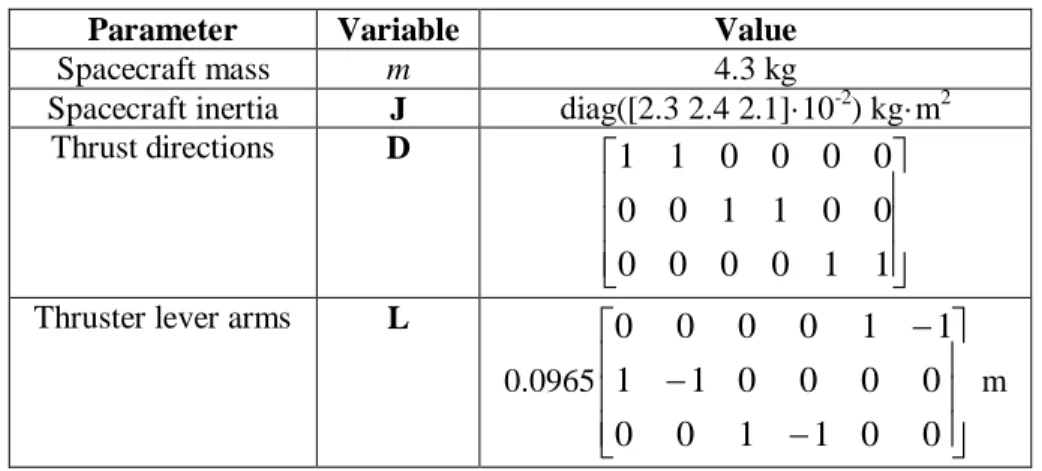
Table 1 gives the values of the 6DOF SPHERES parameters. Note that information for only 6 thrus-ters are given because thrusthrus-ters 7–12 can be paired

with thrusters 1–6, as can be seen in Figure 3. Figure 3. Thruster Locations and Directions

for the SPHERES Satellite. Table 1. 6DOF SPHERES Parameters.

Parameter Variable Value

Spacecraft mass m 4.3 kg

Spacecraft inertia J diag([2.3 2.4 2.1]·10-2) kg·m2 Thrust directions D           1 1 0 0 0 0 0 0 1 1 0 0 0 0 0 0 1 1

Thruster lever arms L

0.0965              0 0 1 1 0 0 0 0 0 0 1 1 1 1 0 0 0 0 m

Baseline Translation. To begin, a simulation of the representative translation with a simple

translational and attitude PD controller and with one thruster failed was performed to demonstrate the need for an improved control system. The control system implemented in this simulation has been used successfully on the ISS for multiple tests (see, e.g., Reference 3). The position control-ler is run at 0.5 Hz and has a damping of ζ = 0.7 and bandwidth of ωn = 0.2 rad/s. The attitude

controller is run at 1 Hz and has a damping of ζ = 0.7 and bandwidth of ωn = 0.4 rad/s. Control

allocation is performed by multiplying the commanded forces and torques with precomputed mix-ing matrix.22

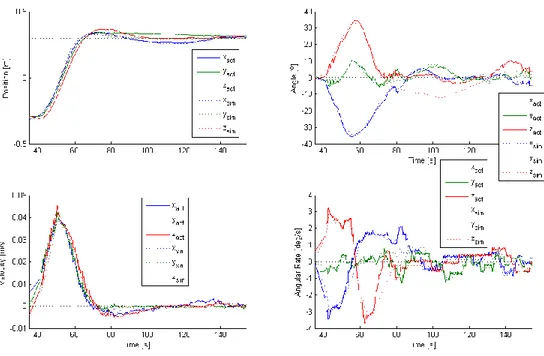
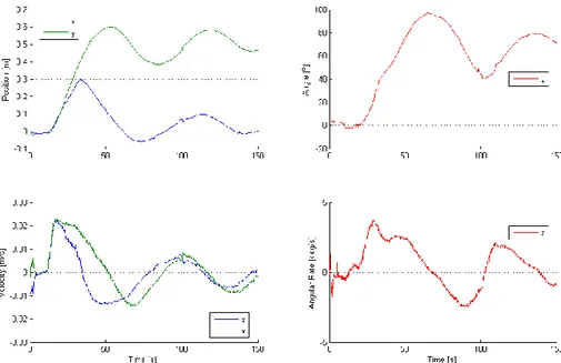
Figure 4 shows four plots of the position, velocity, attitude (converted to roll, pitch, and yaw Euler angles), and angular rates versus time. When the spacecraft approaches the desired position and attempts to stop, thruster 9, which would normally be used to stop the spacecraft fails to ac-tuate. This causes the spacecraft to drift along a curved trajectory away from the desired position. Around 110 seconds, the spacecraft begins to rotate rapidly so that it can once again thrust to-wards the desired position. Around 140 seconds, it reaches the desired position, but once again cannot stop itself and drifts away along a similar curved trajectory. In addition, large oscillations in the velocity and angular rate can be observed, which wastes fuel. This serves as a motivation for creating a control system that can properly handle thruster failures.

Figure 4. 6DOF Maneuver: PD Control, Thruster 9 Failed (Simulation).

Piecewise Trajectory. A simple path planning technique was tested to serve as a comparison

for the MPC algorithm. This method involves piecing together motions that are known to be feas-ible to generate a feasfeas-ible trajectory from the initial state to the final state. To complete the repre-sentative maneuver, the spacecraft rotates about the body x-axis, rotates about the body y-axis, translates to the final position, rotates about the y-axis, and rotates about the x-axis. Nominally, this trajectory avoids the use of thruster 9. The normal control allocator and PD controllers are used in these tests. This test was run on the ISS during SPHERES Test Session 18 on August 15, 2009. Results of this test compared against the simulation are shown in Figure 5. These results show that this technique was able to control the spacecraft from one position to another despite the failed thruster.

The simulation and on orbit data match closely. The only noticeable difference between the simulation and hardware are offsets in time when the various maneuvers start. Since the maneuv-ers terminate based on precise state errors, these differences are expected with slight differences in initial conditions and other noise sources. These results also show that there are low enough disturbances that this technique is valid. If the disturbances were too high, the spacecraft would diverge from its nominal trajectory, which the technique would not be able to correct. Running other cases are not really necessary for this technique since it is a series of decoupled maneuvers. Scaling and rearranging these maneuvers would result in achieving any final position and attitude. With a symmetry argument, it can be shown that this technique can handle any single thruster failure. If this technique was extended to multiple thruster failures, however, it would only handle 43% of all double thruster failure cases and 4.8% of all triple thruster failure cases. This calcula-tion is based on the SPHERES thruster geometry and the fact that this technique requires two body-fixed torques and one body-fixed force. This technique will serve as a baseline to compare the performance of the MPC algorithm against.

Model Predictive Control. Finally, the MPC algorithm was tested in simulation as well as in

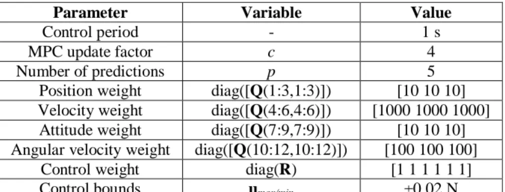
hardware. The tuned parameters that were selected for the MPC algorithm are shown in Table 2. The control loop runs at 1 Hz while the MPC algorithm updates the scheduled controls every 4 control periods (c = 4). With 5 predictions, the MPC algorithm was able to predict 20 seconds in advance (each time step is 4 seconds). The tuned weights and control bounds are also shown in this table. Due to onboard processing limitations of the SPHERES satellites, the algorithm was unable to be run in real-time on the ISS (see Reference 6 for more details). Therefore simulations were run offline to determine the control commands. For the tests on the ISS, these were stored in memory and actuated in an open loop fashion with closed-loop PD controllers keeping the system near the nominal trajectory, which was also stored in memory. These tests were run on the ISS during SPHERES Test Session 24 on October 7, 2010.

Table 2. 6DOF MPC Parameters.

Parameter Variable Value

Control period - 1 s

MPC update factor c 4

Number of predictions p 5

Position weight diag([Q(1:3,1:3)]) [10 10 10]

Velocity weight diag([Q(4:6,4:6)]) [1000 1000 1000]

Attitude weight diag([Q(7:9,7:9)]) [10 10 10]

Angular velocity weight diag([Q(10:12,10:12)]) [100 100 100]

Control weight diag(R) [1 1 1 1 1 1]

Control bounds umax/min ±0.02 N

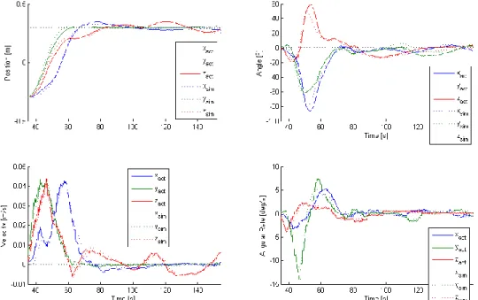
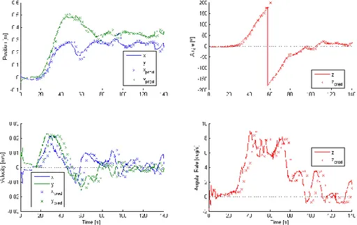
Figure 6 shows the results with thruster 9 failed—again there is good agreement between the simulation and on orbit data. The spacecraft, from the start of its maneuvering, is able to predict that it will not be able to stop properly without thruster 9. Because of this, it begins rotating im-mediately to point other thrusters in the direction of motion so that it can stop its motion towards the desired position. After it reaches the desired position, it is able to rotate back to the desired attitude. Additional simulations with different initial conditions were performed and it was ob-served that the spacecraft was still able to execute the commanded maneuver.

Figure 6. 6DOF Maneuver: MPC, Thruster 9 Failed (Hardware vs. Simulation).

Table 3 shows a comparison of MPC versus the piecewise trajectory technique in terms of several metrics. The first two metrics are the time and fuel used to execute the representative ma-neuver. When using MPC, the maneuver is completed in a fraction of the time it takes to com-plete the same maneuver with the piecewise trajectory technique. This increase in speed comes at the cost of a little more fuel usage. The next few metrics are the percentage of thruster failure cases the technique handles for different numbers of failures. As previously mentioned, for the piecewise trajectory approach these percentages were calculated by determining the thruster fail-ures that could occur while still being able to produce the requisite body-fixed force and torques. For MPC, numerous simulations were run with various thruster failure cases run on the represent-ative maneuver with two different initial conditions. The number of simulations that needed to be run was greatly reduced by using the symmetries of the SPHERES thruster placement. One im-portant note from these simulations is that the weights did not need to be retuned for the various thruster failure cases. The same weights shown in Table 2 were equally valid for the various thruster failure cases. From Table 3, it can be seen that MPC handles a much larger percentage of double and triple thruster failures over the piecewise trajectory technique.

Table 3. Comparison of the Piecewise Trajectory and MPC Techniques.

Metric Piecewise Traj. MPC

Maneuver completion time 90 s 35 s

Maneuver fuel used 2.5% of tank 2.6% of tank

Percent of single thruster failures handled 100% 100%

Percent of double thruster failures handled 42.8% 85.7%

Further hardware testing was performed to determine the effectiveness of the MPC algorithm with multiple thruster failures. Figure 7 shows the results on the representative maneuver, this time with thrusters 1 and 9 failed. Yet again, there is very close matching of the simulation with on orbit data. The fact that all on orbit tests performed closely to the simulation gives high confi-dence in the simulation. The MPC algorithm once again is able to maneuver the spacecraft in a way without using thrusters 1 or 9. The performance in terms of steady state error is slightly worse than the case with only thruster 9 failed.

Figure 7. 6DOF Maneuver: MPC, Thruster 1 & 9 Failed (Hardware vs. Simulation).

Three-Degree-of-Freedom Results

To test unexercised parts of the MPC algorithm, tests were also performed on the 3DOF SPHERES testbed at the MIT SSL. The 6DOF simulation is not a real-time simulation so the ef-fects of finite computation time is not present, disallowing the testing of the delay compensation method. Also, since there is no capability to run the MPC algorithm online on the 6DOF ISS testbed, the MPC algorithm must also be tested on the 3DOF MIT testbed.

The representative maneuver used for the 3DOF tests is similar to that used for the 6DOF tests. The spacecraft starts at a position of r = [0 0]T m and is commanded to move to a position of r = [0.3 0.3]T m, with an initial and final attitude of q = 0°. Table 4 gives the values of the 3DOF SPHERES parameters.

Table 4. 3DOF SPHERES Parameters.

Parameter Variable Value

Spacecraft mass m 12.4 kg Spacecraft inertia J 0.0856 kg·m2 Thrust directions D       1 1 0 0 0 1

Baseline Translation. The first test performed on the 3DOF SPHERES hardware was a

base-line translation with all thrusters operational. The gains of the PD controller were adjusted to match the new mass and inertia of the spacecraft.

Figure 8 shows the resulting trajectory. The satellite clearly is able to complete the maneuver, but there is some steady state error in position. This is actually due to the fact that the table sup-porting the satellites cannot be perfectly leveled. The table legs' length can be adjusted to remove large errors, but small tip/tilt errors might still be present. In addition, the glass on the table is not perfectly flat. This non-zero gradient imparts a force due to gravity on the spacecraft, creating a steady state error in position since there is no integrator in the controller. It is important to recog-nize this source of error because it appears in all of the following results.

Figure 8. 3DOF Maneuver: PD Control, All Thrusters Operational (Hardware).

Figure 9 shows the resulting trajectory when thruster 9 is failed. The behavior is qualitatively very similar to the behavior seen in for the 6DOF case. The spacecraft is unable to stop itself when it reaches the desired position and cannot reach the desired position or attitude after this point. This shows very undesirable behavior that will be fixed by using MPC.

Figure 9. 3DOF Maneuver: PD Control, Thruster 9 Failed (Hardware).

Model Predictive Control. The MPC algorithm was tested on the 3DOF SPHERES testbed

with the parameters given in Table 5. The main control loop was set to run at 1 Hz and the MPC algorithm was initiated every other control period (c = 2), for an effective rate of 0.5 Hz. This algorithm planned 10 time steps in advance (equivalent to 20 seconds since each time step is 2 seconds) and was run online but off-board on a desktop computer. The MPC algorithm took ap-proximately 1.5 seconds to run (per iteration) on a 2.83 GHz processor leaving apap-proximately 0.5 seconds as a buffer for processing time variations and communication delays to and from the spacecraft. Therefore, there is an effective 2 second delay between when the updated controls are requested and when the updated controls are actuated. Table 5 also shows the tuned state and con-trol weights that were used and the concon-trol bounds.

Table 5. 3DOF MPC Parameters.

Parameter Variable Value

Control period - 1 s

MPC update factor c 2

Number of predictions p 10

Position weight diag([Q(1:2,1:2)]) [100 100]

Velocity weight diag([Q(3:4,3:4)]) [100 100]

Attitude weight diag([Q(5,5)]) 10

Angular velocity weight diag([Q(6,6)]) 1000

Control weight diag(R) [1000 1000 500]

Control bounds umax/min ±0.04 N

To test the effectiveness of the delay compensation method, the test was run with and without the prediction step. Note that this ―prediction step‖ is different from the predictive nature of MPC, despite its similar terminology. Without the prediction step, this two-second delay is too large for the controller to handle, causing the control system to not function properly. The result-ing trajectory for this test was qualitatively very similar to that shown in Figure 9.

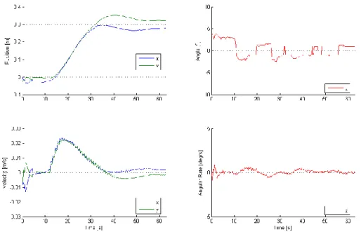
With the prediction step, the two-second delay can be mitigated. Figure 10 shows the resulting trajectory with the predicted states overlayed on the same plot. Ideally, if the model matched the actual dynamics perfectly, the predicted states would match perfectly with the actual states. How-ever, due to process noise, sensor noise and other unmodeled effects, the predicted and actual states to not match exactly. Both the position and angle predictions match well, however there is an obvious delay in the velocity and angular velocity predictions. Despite this error, the predic-tion allows the delay to be compensated enough to achieve stability in the system. The spacecraft is able to reach the desired position by executing an angular flip. The steady state error in position is due to local gradient of the glass table, as was also seen in Figure 8.

Figure 10. 3DOF Maneuver: MPC, Thruster 9 Failed (Hardware).

CONCLUSION

MPC has been applied to solve the problem of controlling a spacecraft that has become unde-ractuated due to failed thrusters. A model of a thruster-controlled spacecraft was developed and analyzed with the sufficient conditions for STLC. For an underactuated spacecraft, the sufficient conditions for STLC were not met. Analysis of the equations of motion and results from this test highlighted the main challenges of controller design for this system: coupling, multiplicative non-linearites, severe control input saturation, and nonholonomicity. MPC has been proposed to solve these challenges. There were several issues with implementing MPC in real time: processing de-lays as well as feasibility and stability. A method for mitigating the processing delay due to solv-ing an optimization problem in real time has been developed. However, the issue of findsolv-ing a feasible solution to ensure stability remains open.

The MPC algorithm was implemented, tested, and compared against a simple path planning technique on the SPHERES testbed. The MPC algorithm performed better than the path planning technique in terms of completion time and number of thruster failure cases handled at the cost of a larger computational load and slightly increased fuel usage. Close agreement of the simulation and on orbit data validated the simulation results. In addition, 3DOF tests on the ground demon-strated the processing delay compensation method since the 6DOF MPC tests could only be run offline.

REFERENCES

1

Tafazoli, M., ―A study of on-orbit spacecraft failures,‖ Acta Astronautica, Vol. 64, No. 2–3, 2009, pp. 195–205.

2

Saenz-Otero, A., Design Principles for the Development of Space Technology Maturation Laboratories Aboard the International Space Station, Ph.D. thesis, Massachusetts Institute of Technology, Cambridge, MA, June 2005.

3

Nolet, S., Development of a Guidance, Navigation and Control Architecture and Validation Process Enabling Auto-nomous Docking to a Tumbling Satellite, Ph.D. thesis, Massachusetts Institute of Technology, Cambridge, MA, May 2007

4

Hughes, P. C., Spacecraft Attitude Dynamics, John Wiley & Sons, Inc., New York, NY, 1986.

5 _{Bullo, F. and Lewis, A. D., Geometric Control of Mechanical Systems: Modeling, Analysis, and Design for Simple}

Mechanical Control Systems, Vol. 49 of Texts in Applied Mathematics, Springer Science+Business Media, LLC, New York, NY, 2005.

6

Pong, C. M., Autonomous Thruster Failure Recovery for Underactuated Spacecraft, Master's thesis, Massachusetts Institute of Technology, Cambridge, MA, September 2010.

7

Murray, R. M., Li, Z., and Sastry, S. S., A Mathematical Introduction to Robotic Manipulation, CRC Press LLC, 1994.

8

LaValle, S. M., Planning Algorithms, Cambridge University Press, New York, NY, 2006.

9

Choset, H., Lynch, K. M., Hutchinson, S., Kantor, G., Burgard, W., Kavraki, L. E., and Thrun, S., Principles of Robot Motion: Theory, Algorithms, and Implementations, The MIT Press, Cambridge, MA, June 2005.

10

Goodwine, B. and Burdick, J., ―Controllability with Unilateral Control Inputs,‖ Proceedings of the 35th IEEE Confe-rence on Decision and Control, IEEE, Kobe, Japan, December 1996, pp. 3394–3399.

11

Sussmann, H. J., ―A General Theorem on Local Controllability,‖ SIAM Journal on Control and Optimization, Vol. 25, No. 1, January 1987, pp. 158–194.

12

Lynch, K. M., ―Controllability of a Planar Body with Unilateral Thrusters,‖ IEEE Transactions on Automatic Con-trol, Vol. 44, No. 6, June 1999, pp. 1206–1211.

13

Lewis, A. D. and Murray, R. M., ―Configuration Controllability of Simple Mechanical Control Systems,‖ SIAM Re-view, Vol. 41, No. 3, September 1999, pp. 555–574.

14

Slotine, J.-J. E. and Li, W., Applied Nonlinear Control , Prentice-Hall, Inc., 1991.

15

Hu, T. and Lin, Z., Control Systems with Actuator Saturation: Analysis and Design, Birkhauser, Boston, MA, 2001.

16

Hu, T., Pitsillides, A. N., and Lin, Z., ―Null Controllability and Stabilization of Linear Systems Subject to Asymme-tric Actuator Saturation,‖ Proceedings of the 39th IEEE Conference on Decision and Control, IEEE, Sydney, Australia, December 2000, pp. 3254–3259.

17

Laferriere, G. and Sussmann, H., ―Motion Planning for Controllable Systems without Drift," Proceedings of the 1991 IEEE International Conference on Robotics and Automation, IEEE, Sacramento, CA, April 1991, pp. 1148–1153.

18

Keerthi, S. S. and Gilbert, E. G., ―Optimal Infinite-Horizon Feedback Laws for a General Class of Constrained Dis-crete-Time Systems: Stability and Moving-Horizon Approximations," Journal of Optimization Theory and Applica-tions, Vol. 57, No. 2, May 1988, pp. 265–293.

19

Mayne, D. Q. and Michalska, H., ―Receding Horizon Control of Nonlinear Systems,‖ IEEE Transactions on Auto-matic Control, Vol. 35, No. 7, July 1990, pp. 814–824.

20

Wie, B., Space Vehicle Dynamics and Control, AIAA Education Series, American Institute of Aeronautics and As-tronautics, Inc., Reston, VA, 1998.

21

Scokaert, P. O. M., Mayne, D. Q., and Rawlings, J. B., ―Suboptimal Model Predictive Control (Feasibility Implies Stability),‖ IEEE Transactions on Automatic Control, Vol. 44, No. 3, March 1999, pp. 648–654.

22 _{Hilstad, M. O., A Multi-Vehicle Testbed and Interface Framework for the Development and Verification of Separated}