An approach to bridging atom optics and bulk spin quantum computation

An Approach To Bridging Atom Optics and

Bulk Spin

Quantum

Computation

by

Kota Murali

Bachelor of Engineering, Bangalore University (2001)

Submitted to the Program in Media Arts and Sciences,

School of Architecture and Planning

in partial fulfillment of the requirements for the degree of

Master of Science in Media Arts and Sciences

at the

MASSACHUSETTS INSTITUTE OF TECHNOLOGY

June 2003

@Massachusetts Institute of Technology, 2003

Author

...

" . . . .

.

.. ... \. ... . . . .

Program in Media Arts and Sciences,

School of Architecture and Planning

May 9, 2003

Certified by

... ?''..

.

. . . .' . .

.

.

....

.:

...

...

...

..

Isaac L. Chuang Associate Professor Thesis Supervisor

A

cce ted by . ...

.... ... ...

/...9

.. .... ... .... ... ... ...

Acc pte by

...

...

...

...

...

...

...

...

...

_{A ndrew B ..Lippm an}

Chairman, Departmental Committee for Graduate Students

MSAHSETTS INSTITUTE OF TECHNOLOGY

JL1 4 2003

LIBRARIES

_

An Approach To Bridging Atom Optics and

Bulk Spin Quantum Computation

by

Kota Murali

Submitted to the Program in Media Arts and Sciences, School of Architecture and Planning

on May 9, 2003, in partial fulfillment of the requirements for the degree of

Master of Science in Media Arts and Sciences

Abstract

This thesis is an exploration in quantum computation and modern physics. Atomic, molec-ular, and optical (AMO) physics, a centerpiece of modern physics, originated in the 1950's with the discovery of nuclear magnetic resonance (NMR), a field which has mostly been left behind in physics. However, NMR has recently taken yet another leap: quantum computers of up to seven qubits in size, the largest realized to-date, have been implemented by apply-ing NMR to molecules in liquid solution. What new lessons can AMO physics learn from these advances made by NMR into quantum computation? And what can NMR quantum computation learn from the many advances made in recent AMO physics? In this work, I study two specific answers to these twin questions: the use of atom-like quantum sys-tems beyond spin-1/2 for NMR quantum computation, and the demonstration of a modern quantum-optical phenomenon, electromagnetically induced transparency, using NMR quan-tum computation. Both examples build on theoretical analysis, and include experimental results, showing how atomic physics could be very useful for implementing certain quan-tum operations and vice versa. These investigations form the basis for an atomic physics test-bed in NMR quantum computation.

Thesis Supervisor: Isaac L. Chuang Title: Associate Professor

An Approach To Bridging Atom Optics and

Bulk Spin Quantum Computation

by Kota Murali

Submitted to the Program in Media Arts and Sciences in partial fulfillment of the requirements for the degree of

Master of Science in Media Arts and Sciences at the

MASSACHUSETTS INSTITUTE OF TECHNOLOGY

June 2003

(2

I' Thesis Advisor...:... .. .. ..~ ~~ ~~~~~.. . . .. .. .. .. . . ... . . . . Isaac L. Chuang Associate Professor Program in Media Arts and Sciences Massachusetts Institute of Technology

T hesis R eader ...

..-

..

o.n

...W augh

Institute Professor Emeritus

Department of Chemistry Massachusetts Institute of Technology

T hesis R eader ... ...

Mildred S. Dresselhaus Institute Professor Departments of Electrical Engineering and Physics Massachusetts Institute of Technology

Acknowledgments

I would like to thank my advisor Isaac Chuang for introducing me to the world of quantum computation, and for his guidance and support all through the work for this thesis. Thanks are due to my thesis readers Millie Dresselhaus for being a constant source encouragement

and inspiration and John Waugh for many useful discussions and advice. I also thank Alex Pines for many useful discussions.

Thank you to the "Quanta" group for its wonderful support. Matthias Steffen, my mentor - a.k.a. "The NMRQC expert", deserves a special thanks for his enormous patience and time introducing me to the spectrometer. Our joint work on most aspects of this thesis are a result of our fruitful collaboration. Thanks to Bin, a very motivated undergraduate student, for working with me on the experiments of chapter 5 of this thesis. His wonderful company and night-outs in finishing up some of the most important simulations for this thesis work is gratefully acknowledged.

Thanks to Andy for keeping the lab in a humorous mood all the time. Aram, the resident (actually non-resident) theorist, of our group for his patience in dealing with my questions. Thanks to Steve has been a wonderful companion of mine both in and outside the lab. Though we did not get a chance to collaborate in research, our collaboration in cooking has yielded very tasty results. Thanks to Josh for teaching me a great deal about quantum dots and also for useful discussions on various aspects of this thesis. Thanks to the Andrew and Francois for their help and support in finishing up this thesis. Thanks to the rest of the Quanta group: Terri, Zilong, and Joshua.

Thanks to my friends in the Gershenfeld group. Ben and Jason have been some of my best friends on campus. Ben introduced me to decoherence phenomena in quantum systems, his contributions are well appreciated which forms the basis for the chapter 4 of this thesis. Thanks to Jason for his help and support all through. The trio of Aram, Ben, and Jason have been very supportive all the time, if not for their help it would not have been possible to lead a sane life here. Thanks to Yael for many useful discussions and for sharing his ideas on building very sensitive NMR probes.

Thanks to my other friends, Maxim, Ajay, Rishi, Ryan, Yu-Ming, Steve, Austin and Muyiwa for their support.

the ever annoying graduate students. Thanks to Mike and Maureen for taking care of us, our experiments could run smoothly only with your help.

Thanks to my parents and sister for their support and encouragement all through my life.

Contents

1 Introduction 19

1.1 Background and motivation . . . . 19

1.2 NMR Quantum Computation and AMO Physics ... ... 20

1.3 Outline of the thesis ... . 22

2 Theory of Quantum Computation 25 2.1 Quantum computing vs. classical computing . . . . 25

2.1.1 Quantum parallelism . . . . 27 2.1.2 M easurem ent . . . . 28 2.1.3 Density Operator . . . . 29 2.1.4 Entanglem ent . . . . 30 2.1.5 Unitary Evolution . . . . 31 2.2

Quantum

gates . . . . 32

2.2.1 Universal Quantum Gates . . . . 32

2.2.2 Single qubit gates . . . . 32

2.2.3 Two-qubit gates . . . . 35

3 Higher-Order Spin Quantum Computation 39 3.1 Introduction . . . . 39

3.2 System of qubits . . . . 40

3.3 Quadrupolar Interaction and NMR . . . . 41

3.4 Single and multiple-qubit gates . . . . 43

3.5 Thermal population distribution and Pseudo-pure states . . . . 46

3.6 Measurement and density matrix reconstruction techniques . . . . 47

3.7 Grover's algorithm speeds up unstructured search . . . . 48

3.7.1 Grover's algorithm: quantum circuit description.. . . . .. 49

3.8 Bloch-Siegert shifts . . . . 50

3.9 Experimental realization of a two-qubit quantum search algorithm using higher-order spin systems.. . . . . . . . 54

3.10 Sum m ary . . . . 55

4 Relaxation Dynamics of Higher-Order Spin Systems 57 4.1 Introduction.... . . . . . . . 57

4.2 The Lindblad Equation . . . . 58

4.2.1 Complete-positivity of Lindblad operators . . . . 59

4.3 Lindblad formulation for higher-order spins . . . . 61

4.3.1 Theory of deriving the Lindblad operators for higher-order spins systems 61 4.3.2 Methods to obtain the relaxation time constants.. . . . .. 63

4.3.3 Phase damping operators . . . . 64

4.4 Experimental realization of relaxation dynamics of an entangled state . . . 66

4.5 Sum m ary . . . . 67

5 Electromagnetically Induced Transparency by NMR 71 5.1 Introduction... . . . . . . . . . . . . 71

5.2 Theory of the EIT effect . . . . 73

5.2.1 Quantum control . . . . 76

5.3 Coherent population trapping using quantum gates . . . . 78

5.4 Experimental realization of EIT in spin systems . . . . 80

5.4.1 EIT in the presence of a strong control field: theory and experimental results . . . . 81

5.4.2 EIT with coherent dark states: theory and experiments . . . . 82

5.5 Ramsey interferometry for measuring phase coherence: theory and experiments 84 5.5.1 Visibility in the strong control field limit: theory and experimental results . . . . 86

5.5.2 Visibility for EIT with coherent dark states: theory and experimental results . . . . 89

5.6.1 Kraus operator formalism for relaxation with a zero temperature reservoir . . . . 92 5.6.2 Simulations using Lindblad operator formalism with a finite

temper-ature reservoir model. . . . . 95 5.7 Sum m ary . . . . 96

6 Conclusions 97

A Simulation for Bloch-Siegert Shifts 99

B Pulse sequence for Grover's algorithm on a spin-3/2 system 105

B.1 Grover Framework . . . . 108 C Lindblad equation for higher-order spin systems 121

D Simulation for Ramsey interferometry 125 D.1 Pulse sequence for EIT in the strong control field limit . . . . 130 D.2 Pulse sequence for EIT using coherent dark states . . . . 132

List of Figures

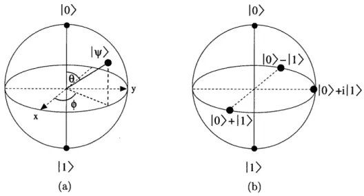
2-1 (a) Bloch sphere representation of an arbitrary quantum state

1t)

for a single qubit. (b) Representation of several important quantum states, ignoring the normalization factor. . . . . 26

2-2 Quantum circuit representation of (a) an arbitrary single qubit rotation U, and (b) the NOT gate. . . . . 35

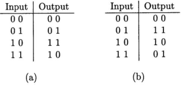
2-3 Truth tables for (a) the CNOT12 gate, and (b) the CNOT2 1gate . . . . 35

3-1 Schematic energy level diagram for an I = 3/2 system with quadrupolar

splitting. The energy levels correspond to the spin states I = 3/2, m = -3/2), 1I = 3/2,m = -1/2), |I = 3/2,m = 1/2), and |I = 3/2,m = 3/2), and can be assigned the logical labels |00), |01), 110), and 11) respectively.

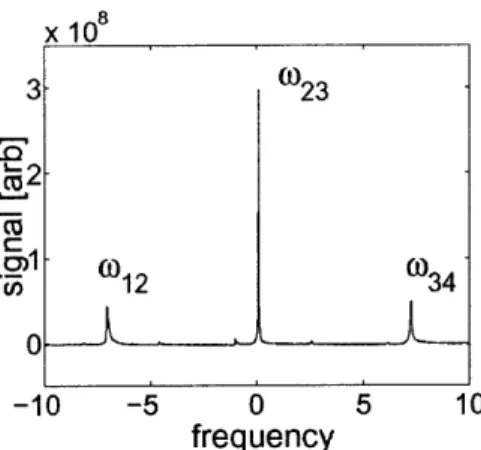
3-2 An NMR spectrum of a spin-3/2 system displaying the three allowed

transi-tions: 3/2 -+ 1/2, 1/2 -+ -1/2, and -1/2 -+ -3/2 denoted as W12, W23, and

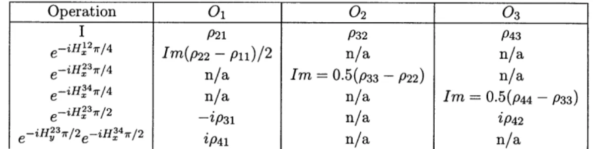
3-3 Illustration of how to implement a universal set of quantum gates in an

I = 3/2 system. Time goes from left to right. The first and third column

show qubit operations with the horizontal lines denoting the qubits, and the subscript denoting the rotation angle in units of ir/2. Columns two and four show the corresponding transition selective operations for the I = 3/2 system, where the first line denotes the transition at frequency W12, and so forth.

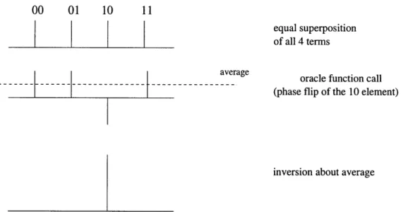
Single qubit Y-rotations are implemented similar to the shown X-rotations. From these, single qubit Z-rotations can be implemented. Together with the controlled Za-gate, arbitrary 4x4 unitary gates can be implemented. .... 44 3-4 Pictorial description of Grover's algorithm using inversion about the average

principle. Here, the vertical lines labeled as |00), |01),

110),

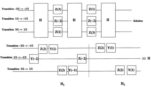
and |11) indi-cate the probability amplitudes of the respective states. The solution to the problem, in this case involving four elements is found in one iteration as seen in the figure. . . . . 50 3-5 A transition circuit model of a particular instance of Grover's algorithm.

Here, Z(x) indicates Z for duration x in units of 7r/2, H indicates a HADAMARD transform on both the qubits, that is implemented by the sequence of pulses shown described in equation 3.10 and 3.11. The transition circuit of the

HADAMARD gate is shown as a concatenation of H1 and H2, HADAMARD

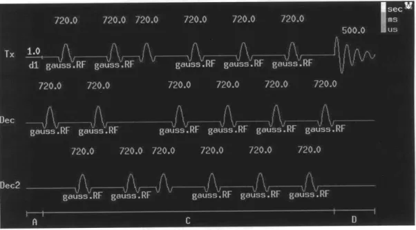
gates on the first and second qubit respectively. . . . . 51 3-6 Typical pulse sequences based on the transition circuit model of the

spin-3/2 system for a Grover iteration. Here gauss.RF indicates Gaussian shaped pulses of duration 720ps duration. Tx, Dec, and Dec2, denotes the RF channels used for manipulating -3/2 -> -1/2, -1/2 -> 1/2, and 1/2 -+ 3/2

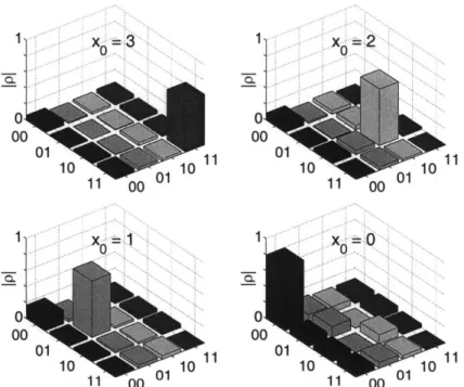
transitions, respectively. dl denotes the delay before the pulse sequence starts, typically used to have a delay between experiments. The decaying sine wave of 500 ms indicates the acquisition period. . . . . 52 3-7 Plot of the absolute value of the traceless deviation density matrices for

zO = 3, xo = 2, xo = 1 and xo = 0. For visual clarity, each plot has been

adjusted such that the minimum diagonal value equals zero. . . . . 55

4-2 (a) Schematic energy level diagram for an I = 3/2 system with quadrupolar splitting. The energy levels correspond to the spin states |I = 3/2, m = 3/2),

|I = 3/2, m = 1/2), 1I = 3/2, m = -1/2), and 1I = 3/2, m = -3/2), and can be assigned the logical labels 00, 01, 10, and 11. (b) Thermal spectrum of

Cs133 displaying the three allowed transitions. . . . . . . . . 62

4-3 Schematic showing a quantum circuit used to create an entangled state. . . 66

4-4 Simulations of the relaxation dynamics of an entangled state based on the Lindblad equation. Each plot shows the absolute value of the traceless devi-ation density matrix adjusted by an identity element such that the smallest element along the diagonal is zero. Here time goes from left to right. ... 68

4-5 Snapshots of experimentally reconstructed dynamics of the density matrix evolution of the entangled state. It is clear how the system evolves from the point it is prepared to a time corresponding to the maximum of the T relaxation times. We clearly see the population distribution approaching the thermal equilibrium distribution rhoeq (see Eq.( 4.15). Here the labels 1, 2,

3, and 4 stand for 100), 101), 110), and |11) respectively. Time goes from left

to right. . . . . 69

5-1 (a). Energy level diagram of A-like spin states of a three-level atomic system.

(b). Schematic energy level diagram for the I, = -1/2,1/2, 3/2 levels a

multi-level system with quadrupole splitting . . . . 74

5-2 Experimental data verifying the transparency behavior of an NMR EIT

sys-tem in the strong control field limit described in section 5.4.1. Here, we observe the signal corresponding to 11) (21 element of the density matrix. The intensity of the probe field was set to a strength equivalent to ir units. The dash-dot line represents the 1/b trend of Rabi oscillations in the 11) (21 ele-ment as derived in Eq.( 5.3). The dotted line is the simulation result, which includes the RF inhomogeneity of the control field and the Bloch-Siegert shifts (see appendix A). The points are the experimental results obtained by

averaging over five experiments. The height of the error bars were obtained from standard deviations normalized by Nexperiments - 1, where Nexperiments is the number of repeated experiments. . . . . 82

5-3 Experimental data verifying the transparency behavior of an NMR EIT

sys-tem in the strong control field limit, just as in Figure 5-7. Here, the intensity of the probe field was set to a strength equivalent to 37r/2 units. . . . . 83

5-4 Experimentally reconstructed deviation density matrix of the "dark state"

11-3) _{(a) before applying the EIT Hamiltonian and (b) after applying the}

EIT Hamiltonian for a duration equivalent to 37r/2 pulses. Note that the

density matrices presented here show only the absolute values of the elements for the sake of visual clarity. . . . . 84

5-5 (a). Energy level diagram of A-like spin states of a three-level atomic system

coupled to an additional reference level |R). (b). Schematic energy level diagram for the Iz = (-3/2, -1/2, 1/2, 3/2) levels a multi-level system with

quadrupole splitting. . . . . 85 5-6 Simulations and experimental results of visibility as a function of b/a in

the strong control field limit. The solid line indicates the ideal expectation of visibility, the dashed line indicates the simulated behavior including decoher-ence effects and pulse imperfections, and the points indicate the experimental results. The experimental results are in close agreement with simulations. . 88 5-7 The expectation of the reference state |R) as a function of 0. The solid

line indicates the ideal value in the expectation of |R), the dashed-line the simulated expectation of

IR)

including decoherence effects and the squares indicate experimental results. They show the characteristic cos2 _{0 behavior}

derived in Eq.( 5.32). . . . . 89 5-8 Visibility of of the expectation value of

|R)

state as a function of b/a for

EIT with a coherent dark state. The solid line is the ideal case scenario, the dashed-line indicates simulated expectation with decoherence effects and the

points indicate experimental results. Here, the dark state is

1)-13

,

while the

ratio b/a is varied with a fixed probe field and varying control field. .... 91 5-9 Quantum circuit implementing the Ramsey interferometry experiment on a

spin-3/2 system. Time goes from left to right, t, indicate the time period for which the respective gate p is applied.. . . . . . . . . 92

5-10 Simulations and experimental results of visibility as a function of b/a in the strong control field limit using Kraus operators given in Eqs.( 5.45) and ( 5.46). The solid line indicates the ideal expectation of visibility, the dashed line indicates the simulated behavior including decoherence effects and pulse imperfections, and the points indicate the experimental results. . . . . 93

Chapter 1

Introduction

1.1

Background and motivation

Computation is an active area of thought and practice the human race has intensely pursued to make many of its tasks in life simpler. This pursuit is clearly seen from the theoreti-cal and technologitheoreti-cal advances made in inventing algorithms and building computational devices. The theoretical challenges in algorithms include finding ways of solving computa-tional problems using minimal resources such as space and time. While the technological advances are largely due to the astonishing progress made in semiconductor physics and integrated circuit technology. It is inferred from Moore's law that the size of the transistor will soon reach atomic dimensions. At these extreme regimes of nature the dynamics of these devices would be governed by quantum mechanics and hence computational processes become quantum mechanical.

In the early 1980s Feynman [Fey82] sought to see if quantum mechanics could be useful for fundamentally reducing the amount of resources required for computation. This remark-able speculation turned into reality when Deutsch [Deu85] invented an algorithm that ex-ploits quantum mechanical properties to solve a certain class of computing problems. These first few bold steps gave birth to a totally new paradigm in computing known as quantum computation. Quantum computing was mostly a theoretical fancy until the invention of the celebrated Shor's algorithm [Sho94] for prime factorization, which showed that quantum computers could exponentially outperform known classical algorithms. This was followed

by the invention of Grover's algorithm [Gro96], which can search an unsorted database

of activity in building quantum computers and construction of a new class of quantum algorithms among physicists and computer scientists. The first experiments for building quantum computers started with Cirac and Zoller [CZ95] showing the implementation of quantum logic in cold trapped-ions. This lead to a flurry of other experimental proposal for building quantum computers based on ion-traps[MMK+95], NMR [GC97], Phosphorus-doped silicon substrates [Kan98], quantum dots [DSS98], superconducting circuits [MOL+] and electron-spin resonance transistors [V+00]. The first experimental implementation of quantum algorithms by NMR was proposed by Gershenfeld and Chuang [GC97] and Cory, Fahmy, and Havel [CFH97]. Of all the above proposals, NMR has made the most progress as nuclear spin states have long coherence times in molecules and the state of art NMR spectrometers being the most advanced of all. To date, NMR quantum computation has demonstrated Grover's algorithm [CGKL98, VSS+00] and Shor's algorithm [VSB+01] using a 7-qubit quantum computer. In spite of this, higher number of quantum bits using NMR is going to be hard to come by as obstacles like decoherence times and signal-to-noise pose an unsurmountable challenge with the size of the molecules. It is believed that solid-state approaches using quantum dots [DSS98] and superconducting circuits [MOL+] might be well suited for scaling up though enormous experimental challenges need to be overcome in these areas.

In this thesis, we explore other interesting possible schemes to extend the range of present day NMR quantum computers. Another interesting area that we explore is the connection between NMR quantum computing and Atomic, Molecular and Optical (AMO) physics. AMO physics has been envisioned for many applications in storing quantum mem-ory [HHDB99, LDBHO1, PFWL01] for long distance quantum communications. We show that AMO phenomena can be implementing in spin systems using NMR, thus laying a foundation for implementing AMO phenomena in NMR-based systems.

1.2

NMR Quantum Computation and AMO Physics

Almost all experimental implementations [CGK98, CGKL98, CVZ+98, JM98] so far have used spin-1/2 systems in external magnetic fields, where the two energy states of the nuclear spin are treated as a quantum bit. Many such coupled spin-1/2 nuclei can be treated as multi-qubit quantum computers and have been used to realized quantum logic and

algo-rithms. As described earlier, it is hard to build bigger NMR quantum computers as the decoherence times and signal-to-noise ratio get smaller with the size of the molecules. If this is the case how do we extend the range of NMR quantum computers?

Higher-order systems offer some viable alternatives to spin-1/2 NMR quantum comput-ing. Higher-order spin systems have been extensively studied because they offer intriguing alternatives to two-level quantum systems. Some of the advantages of higher-order spins are: certain quantum operations are significantly easier to implement in higher order spin systems as compared to two-level systems [Fun0l] , several of them coupled together could scale and might be well-suited for building NMR quantum computing systems containing more quantum bits than is currently possible, it might be possible to polarize a quadrupo-lar system to much higher levels than is currently possible with spin-1/2 systems [VLV+01] which can improve the signal-to-noise obstacle, and it might be possible to build quantum computers using nuclear spins without external magnetic fields [FG02).

We mainly focus on the following two topics in quantum computing: implementing quantum algorithms using atom-like higher-order spin systems, and their characterization

by relaxation models. As we discussed above, higher-order spin systems offer some intriguing

alternatives to extend the range of NMR quantum computing [Fun0l, KSM+02]. Integrating higher-order spins systems with regular NMR quantum computing systems might help in taking advantage of their unique features in implementing certain quantum gates. As a step in this direction we demonstrate the implementation of universal quantum computing on higher-order spin systems and incorporating these universal gates to implement a two-qubit Grover's quantum search algorithm. This is the first demonstration of a quantum algorithm on a higher-order spin system.

It is also important to characterize the interaction of quantum systems with their envi-ronment, since parameters like coherence times are only an indirect measure of how strong the system-environment interaction is. These coherence time parameters finally decide on the viability of a quantum system for quantum computation. As a step in this direction, a model describing the relaxation processes in higher-order spins is constructed. This the-oretical model is extensively tested by experiments on the relaxation of certain quantum states.

Another very interesting question we address is if such higher-order spin systems can be used to demonstrate other physical phenomena by NMR. If so what are they?

Higher-order spin systems show a very close resemblance to AMO quantum systems. One would therefore be immediately tempted to ask if AMO phenomena can be simulated in NMR systems? We demonstrate that this is indeed the case by experimentally implementing the Electromagnetically Induced Transparency (EIT) effect in spin systems. This forms a basis for bridging the two seemingly distant areas of AMO physics and NMR quantum computa-tion. Such bridges between quantum computation and other areas of physics demonstrate that quantum computing can be a very powerful tool for gaining an intuitive understanding physical phenomena and learning how to control them. These investigations open up a whole new range atomic physics tests based on NMR quantum computation. This thesis addresses the above described issues in NMR quantum computing and AMO physics.

1.3

Outline of the thesis

This thesis broadly deals with higher-order spin quantum computing and its relation to AMO physics.

In chapter 2, we begin by introducing the notion of quantum bit and comparing quantum and classical computations. We show the ways in which quantum computation is much more powerful than its classical counterpart. Then, by means of describing the postulates of quantum mechanics and some mathematical preliminaries, we show how quantum systems can be manipulated to implement universal quantum gates.

In chapter 3, we show the use of higher-order spin systems as alternatives to spin-1/2 systems by experimentally realizing the quantum search algorithm on a spin-3/2 system. We show this by developing techniques for universal quantum computing using higher-order systems and then incorporating this universal set of quantum gates to implement the required unitary transforms for the quantum search algorithm. The results are verified for all the possible cases of a two-qubit search algorithm and experimentally reconstructing the density matrices corresponding to the solutions to the problem. This is the first complete implementation of a quantum algorithm on a higher-order spin systems.

In chapter 4, we study the effect of environmental interaction on higher-order spin systems. We introduce the Lindblad formulation of decoherence in these spin systems, and calculate the required amplitude and phase damping operators for characterizing the system-environment interaction. We compare our formulation with simulations and experimentally

reconstructed density matrices for the relaxation of an entangled state. This model is extensively tested in modeling the decoherence of the EIT experiment on higher-order spin systems.

Finally, in chapter 5, we demonstrate the realization of the EIT effect in spin systems.

A spin-1 system is treated like an AMO system to experimentally realize EIT by NMR. The

transparency behavior is tested by experimentally reconstructing the evolution of the density matrix and measuring the phase evolution of the dark state through Ramsey interferometry.

Our experiments form the basis for an AMO test-bed in NMR quantum computing. We conclude in chapter 6 by summarizing our experiments with higher-order spin sys-tems for quantum computing and AMO physics experiments by NMR.

My specific contributions in this thesis work:

1. In chapter 3 are: to formalize the appropriate Hamiltonians to derive the necessary

single-qubit and two-qubit operations (universal quantum gates) for a two-qubit spin-3/2 system. The derived operators were then used to realize the required unitary operators for the two-qubit Grover's algorithm. I jointly developed density matrix reconstruction techniques for higher-order spin systems, these techniques were used for the final read-out of Grover's search algorithm.

This part of the thesis was a joint work with my mentor, Matthias Steffen, a final year graduate student in the Quanta group. He introduced me to the NMR spectrometer and taught me techniques to implement quantum algorithms on NMR spin systems. We jointly set up the experiments and found the required pulse sequences for Grover's algorithm on a spin-3/2 system. The C code for the framework for this work was written by Matthias; this was not within my expertise at that time as I was new to working with the spectrometer.

As a fresh graduate student, this interaction helped me a lot in setting up experiments on my own for the work described in chapters 4 and 5.

2. In chapter 4 are: constructing the Lindblad operators for relaxation in higher-order spin systems. I set up experiments to test the formulation by observing the relaxation dynamics of a spin-3/2 system. The theoretical formulation and simulations was a result of joint work with Ben Recht, a third year graduate student in the Physics and Media group at the Media lab. The experiments were done on my own, after gaining experience handling the spectrometer with work done in chapter 3.

I tested this formulation by experimentally implementing these dark states on a spin-3/2 system. The theory for EIT in strong control field limit was suggested by my advisor Isaac Chuang and the experimental realization was done through a collaborative effort with Hyung-Bin Son, and Matthias Steffen. Bin was an UROP student working with Matthias and me for his bachelor's thesis in physics. The theory and experiments on Ramsey interferometry to observe phase coherence of the NMR EIT system was a joint work between the three of us. The simulations to estimate visibility of the EIT system including relaxation effects were based on the Lindblad model developed in chapter 4. The simulation model is in good agreement with experimental results for visibility. With this, our model has undergone rigorous tests in estimating decoherence of a higher-order spin system, thus confirming the relaxation model. The simulation code attached in appendix D were written by Bin and me.

Chapter 2

Theory of Quantum Computation

In this chapter, we introduce the notion of quantum bits and their mathematical description. We discuss some of the known key points that make quantum systems much more powerful than classical computers. A systematic study of these topics provides fertile ground for thinking of building a workable quantum computer. We introduce the language of quantum bit manipulation which forms the basis for a quantum circuit model of algorithms that is extremely useful as a step by step approach to working with a quantum computer.

2.1

Quantum computing vs. classical computing

Classical vs. quantum bit

A classical bit is represented by the logical binary values 0 or 1 and can be represented by

any physical system that has at least two distinguishable states. The on or off states of a

transistor, represented by voltage, or the orientation of the domains of magnetic particles are examples of many physically measurable quantities of physical systems.

A two-level quantum system such as a spin-1/2 nucleus or a polarized photon can be

used as a quantum bit. The two distinguishable computational basis states can be labelled as

10)

and |1) to encode the logical values 0 and 1 respectively 1. In general, a quantum system can be represented as a superposition of its basis states. This is mathematically represented as,

1) = colo) + cill) (2.1) 'The 1) symbol denotes the quantum mechanical state of the system in the Dirac notation.

where co and ci are complex numbers that satisfy the normalization condition

Ico

2+

Ic1

2

1. For the sake of convenience in representing this state on the Bloch sphere, we can rewrite

the above state as,

|@) = cos(9/2)|0) + e-'sin(0/2)|1) (2.2)

The above form can be conveniently represented as a vector on the Bloch sphere as shown in Figure 2-1. This picture is very useful in understanding the dynamics of spin systems in the context of NMR quantum computing. Now suppose we have two qubits. The quantum

10>

10>

|1)

(a)

0>+il

1>

|1)

(b)

Figure 2-1: (a) Bloch sphere representation of an arbitrary quantum state |@) for a single qubit. (b) Representation of several important quantum states, ignoring the normalization factor.

state

l|0)

can be written as:

1@) = coo 100) + coi 101) + cio110) + cuil11) (2.3)

where 100) is the shorthand notation for (10) | 0)), in which 0 is the symbol for tensor

condition. A general two-qubit state can be compactly represented in matrix form as, Coo () = c2.4) C1 0 LC_{1 1}

In the same manner, an n qubit quantum state IV)) can be described as: 2"-1

|$)E= Zcili) (2.5)

i=O

where i is the decimal representation of the quantum state, and the ci satisfy the normal-ization condition .2n-1| c 12 = 1. Describing the state of n qubits, in general, requires

2" complex numbers. An n qubit system can be in 2" states at once, thereby making it an exponential resource for storing information. This is in sharp contrast to a string of n classical bits that can hold only one state at once. This is our first hint of how quantum resources outperform classical resources.

2.1.1 Quantum parallelism

Now that we have understood the superposition principle, imagine a computing device that can take quantum states as input. Suppose we compute the function f(x) when

I

x) = co0) + cill). Because quantum mechanics is linear, the function acts linearly on the

superposition of states, we obtain the following transformation:

colo) + c1|1) -> coif (0)) + cif(1)) (2.6)

Even though we applied the gate f(x) only once, it has been computed for two values, x = 0

and x = 1, at the same time. Similarly, let us consider a two-qubit input. If we prepare the

input state into the superposition,

then the execution of f(x) results in the output state:

coo lf (00)) + coilf(01)) + ciolf (10)) + cnlf(11)) (2.8)

Now, f has been been evaluated four times in parallel. In general, for every added input qubit, we double the number of parallel computations. Thus, a function with n possible input qubits, can be evaluated for all 2" input values at the same time:

2n-1 2n-1

S

cxIx) -4

5

cXIf(x)) (2.9)

x=0 x=0

where x is an integer encoded by n qubits. While the number of parallel computations on a classical computer can only grow linearly with their size,

a quantum computer can perform an exponential number of computations in

parallel.

This spectacular feature was first introduced by David Deutsch who coined the term

quan-tum parallelism [Deu85] to describe it.

As a consequence of quantum parallelism, computers which rely on qubits in a superpo-sition would appear to be exponentially more powerful than classical computers. However, this would only be true if we can also readout this information. Otherwise, the computa-tion is meaningless. This brings us to understanding the measurement postulate in quantum mechanics.

2.1.2 Measurement

Measuring a quantum system, or "looking" at it to determine in what state it currently exists can be described as a "disturbance" which causes a system to jump to an eigenstate of the dynamical variable that is being measured. Consider the case in which we have a quantum system in a superposition of the basis states

10)

and 11),

|) = colo) + ciii) (2.10)

Measuring this system |') in the computational basis

10)

and 1), makes the system collapse to the state 10) with probability

Ico1

2

mentioned before, even though we have an exponential increase in resources due to quantum parallelism, the outcome of the exponential computations is not accessible. Here is where quantum interference comes into play. We would like to evolve our system in such a way that unwanted terms are reduced to vanishingly small probabilities due to interference and we are left with the solution states with high probability. This is the heart of any quantum algorithm and we will show this when we describe Grover's algorithm in chapter 3.

2.1.3 Density Operator

Here we introduce some more important mathematical objects, that help to characterize quantum systems completely. One such operator is the density operator. It is defined as the outer product of the quantum state, and represented as,

p=

I|0)(0I

(2.11)

To get a feel for the power of this operator, let us consider a quantum statistical mixture of states and a pure state. We can conveniently describe a mixed state by introducing the

density operator p:

p

=

Zpi;$i)(Oi

(2.12)

where (01 is the Hermitian conjugate of 1') and

E>p;

= 1 with p; 0. The density

operator of a pure state is then just p = 10)(V51. The density operator has two important characteristics:

Tr(p) = 1 (2.13)

because Tr(p) =

EZpiTr(|$i)(4i)

=

E>pi,

as any quantum system has to conserve prob-ability. Here, Tr represents the trace of a matrix. Furthermore, the density operator is a

positive operator as (#|pl#) 0, where 1#) is any quantum state. Since a pure state has

only one eigenvalue, necessarily equal to unity, and a mixed state has at least two non-zero eigenvalues, we can derive a very useful condition which allows us to distinguish mixed and

pure states2:

Tr(p2) = 1 -> when p is pure

Tr(p2) < 1 -> when p is mixed

A quantum system can only be in one single quantum state however. What then is the

physical representation of mixed states? A mixed state is a manifestation of the lack of knowledge about the quantum system or an ensemble of quantum systems. For example, all NMR quantum computers at present consist of about 1018 quantum computers acting in parallel, yet not all of them start out in the same state, thus requiring a description using mixed states. It will be clear later how exactly we can still do quantum computing by NMR. With the tools we have learnt so far, we are now ready to understand the dynamics of the time evolution of quantum systems.

2.1.4 Entanglement

For any given bipartite pure state

|@AB),

we can associate a number known as the Schmidt number, which is the number of non-zero eigenvalues of the reduced density matrix PA (or

PB). In terms of the Schmidt number, we can define entanglement as: |@AB) is entangled

(or non-separable) if its Schmidt number is greater than one; otherwise the quantum state is separable (or unentangled). Thus a separable bipartite pure state is a tensor product of pure states,

kbAB) =)A (9 )B (2.14)

The reduced density matrices of such a quantum state, PA = kb)0kA and PB B B > which are pure state density matrices. Hence the Schmidt number is one. Any state that

can not be expressed as such a tensor product is entangled, which means PA and pB are mixed states.

Consider the state IOAOB+IlAl) , measuring the state of the first qubit collapses the

state of the second qubit into the exact same state as the measurement outcome on the first qubit. It is rather non-intuitive that measurement of one system influences the state of the

2

other system with which it is interacting! Such a state is also known as the Bell state or

EPR pair [Bel66, EPR35] Entanglement seems to be a necessary condition for speeding up

quantum algorithms.

These non-local effects make quantum information very powerful. There are two impor-tant applications of these non-local effects. 1. Superdense coding where two bits of classical information can be transmitted by sending one qubit which is a part of an entangled pair. 2. Teleportation is the other, where a quantum bit can be teleported using an entangled pair and two bits of classical communication [BBC+93].

2.1.5 Unitary Evolution

Schr6dinger's equation governs the dynamics of any quantum system. The time evolution of a system can be written as,

dl@~,(t))

ih dt = XH (t)|4(t)) (2.15)

dt

where h is Planck's constant, and H is the Hamiltonian that describes the total energy of the quantum system. When the Hamiltonian is time-independent, this equation has an easy solution:

IV)(t))

=

exp

( )

I(0))

(2.16)

The operator that evolves the initial state 10(0)) to the final state 1|0(t)) is a unitary operator U, due to the fact that H is Hermitian.

U = exp (2.17)

Hence, U is reversible and so is quantum computing. Reversible computers have been shown to compute without any energy dissipation. The class of universal gates for reversible computing is a subject of its own. We refer to [Lan6l, Ben73] for more on this. The results from reversible computing form a basis for universal quantum computing as quantum computation is inherently reversible.

Another useful form of unitary evolution in terms of the density operator can be written as,

p(t)

=

[pilOi(t))(Oi(t)|

=

piUlIi(0))(V@i(0)|UI

=

Up(O)Ut

(2.18)

These two forms of time evolution of quantum systems are to be our language of describing the evolution of qubits and will be used often in the sections to follow.

2.2

Quantum

gates

In this section, we describe a set of unitary gates with which we can construct any arbitrary quantum circuit. We discuss the notion of universality and describe a set of universal gates which are straightforward to implement on an NMR quantum computer. We then show an example of decomposing a simple two-qubit unitary transform into a sequence of universal gates. These concepts help us develop ways to perform quantum computing on other quantum systems, which we will describe in building a working model of a higher-order spin quantum computer in chapter 3.

2.2.1 Universal Quantum Gates

One of the most important results from classical theory of computation is that any boolean logic circuit can be implemented from a finite set of boolean operations. This set of opera-tions or gates is known as a universal set of gates. In classical circuits, the NAND gate is in itself universal and so is the NOR gate.

Along similar lines, any arbitrary unitary operation can be approximated from a finite set of quantum gates. These gates are arbitrary single qubit operations and the controlled-NOT (CNOT) gate. We will begin constructing this universal set by describing single qubit gates. It should be noted that this is not the only universal set of quantum gates. This set is convenient for us in terms of implementation and hence use it as our universal basis.

2.2.2 Single qubit gates

It is convenient to describe qubits and their unitary evolution in matrix notation. For example, a qubit in a superposition of its basis states can be written as,

|@) _(2.19)

where IV)) is a column vector of two entries, co and cl which are the amplitudes of the |0) and 1) states respectively. A single qubit unitary matrix acting on this state is simply a

2x2 matrix:

|)final = Uinitial (2.20)

For example, consider the NOT gate that takes

10)

-4 1) and |1) - |0):

UNOT

=

0

1

(2.21)

1 0

By applying UNOT as shown in Eq.(2.20), we get:

|)n = 0 1 co ci (2.22)

1 0 ci co

We can see that the amplitudes for the

10)

and

|1)

states are switched, as expected. The NOT gate is a very simple example to understand the matrix formulation of unitary evolution of a quantum system. In general, any single qubit rotation is of the form,

U = esaR1(#) (2.23)

where Rf1(f3) corresponds to a rotation of the state vector [@) on the Bloch sphere in Figure

2-1 around the axis

nt

= (nx, ny, nz) over an angle 3, here, eia represents the overall phase of the unitary transform. Mathematically, we can define R1 as

Rn(#) = exp - 2t = cos(3/2) I - i sin(3/2)[no-x + nyo-y + nzz] (2.24)

where a = (o-, 0-y, o-z), with o-x, oy, az denoting the Pauli matrices and I the identity matrix:

0 1 0 -i 1 0 1 0

Ux=[

]

,

],

-z[

=

,

1

(2.25)

1 0 i 0 0 -1 0 1

The Pauli matrices satisfy the following useful relationships:

There are three important single qubit rotations -the 1,

Q

and i-rotations. These are given

by:

cos(22) -i sin(22)

Rj(#) = cos(f/2) I - i sin(#/2) o-.

[

,

(2.27)

-isin (,) cos(O)

[cos(2)

-sin()1

Ry (#)

=

cos(#/2) I - i sin(#/2) a- =

,o2)

(2.28)

sin(o) COS (,)

R2(#) = cos(/3/2) I - i sin(#/2) o-z =J . (2.29)

0 e f

Note that the NOT gate can be constructed by applying Rg(180_{') up to an overall phase.}

From these s,

9

and i-rotations, we can implement any rotation about an arbitrary rotation axis, because we can write any U as:

U = e-mRz(#)Ry(-y)R(6) (2.30)

We actually do not require the ability to perform explicit i-rotation because we can generate it from concatenating i- and

Q-rotations:

Rj(3) = Rj(900) R (0) Rj(-900) (2.31)

where time goes from right to left (i.e. the rotation over -900 is applied first). Thus, arbitrary - and

Q-rotations

are sufficient to implement any arbitrary single qubit rotation U. One additional and important single qubit gate is the HADAMARD gate, defined as:

H = _(2.32)

v'- _{1 -1}

This gate allows us to put a qubit starting in the |0) state into an equal superposition of the basis states as it applies the transformation

10)

, and |1) - 0" . The HADAMARD

gate can be implemented via - and

Q-rotations:

When we have multiple qubits, the single qubit operations can be written in the Kronecker product notation. Below is an example of a single qubit operation on the third qubit in a three qubit system.

R4(#)

=

exp -i

2

o

exp,

2D

(2.34)

where IIX is just the shorthand notation for 1 @ I o-x and I is the 2 x 2 identity matrix. We can describe these single qubit rotations via the quantum circuit language, first introduced by Deutsch

[Deu89]

and shown in Figure 2-2. The horizontal wires denote the individual qubits, and time goes from left to right.

U

(a) (b)

Figure 2-2: Quantum circuit representation of (a) an arbitrary single qubit rotation U, and (b) the NOT gate.

2.2.3 Two-qubit gates

Now that we have learnt the mathematical description for single qubit operations, we only need to describe the two-qubit CNOT (controlled-NOT) gate, and we are ready to implement any arbitrary n-qubit operation. The truth tables for the two-qubit CNOTij are shown in Figure 2-3 where i is the control bit and

j

the target bit. In other words, bit

j

is flipped only if bit i is in the logical state 1 (or the quantum state |1)).

Input Output Input Output

00 00 00 00

01 01 01 11

10 11 10 10

11 10 11 01

(a) (b)

Figure 2-3: Truth tables for (a) the CNOT1 2 gate, and (b) the CNOT21 gate.

on an arbitrary two-qubit state |@). Similar to Eq.( 2.19), |@) is now a column vector with four entries: coo |@)initial = Co C1O Lc"1 (2.35)

Using the truth table from Figure 2-3 and applying CNOT12 to

I)),

the output will be:

Coo

final Coi Ucnoi12

C1 1

c O

The unitary matrices for the CNOT gates are then:

1 0 0 0 0 1 0 0 0 0 0 1 0 0 1 0 and Ucots₂ = Coo Coi CiO C1 1 1 0 0 0 (2.36) (2.37)

The CNOT gate is implemented using a combination of single qubit operations and the evolution of the coupling Hamiltonian. As an example, we consider a two spin system with scalar or J-coupling between the spins, the unitary evolution of this interaction can be described in the matrix form as,

Uj(t) = exp (-iirJo-z1o2t/2) =

e-i-Jt/2 0 0 e+iiJt/2

0

0

0

0

e+irJt/2 0 0 e-irJt/2

where J indicates the strength of the scalar coupling. An approximate CNOT gate can be

(2.38)

obtained by applying the following sequence of X, Y, and J evolutions, 1 0 0 0 0 i 0 0 Ucnot2 = Y2Uj(1/2Ji2)X2 = 0 0 0 1 (.9 0 0 -i 0

where, Y2 indicates a ir pulse along -Y axis. Here time goes from right to left. This unitary

transformation is an approximate CNOT gate due to the presence of additional phases. These phases can be removed by applying z-rotations as shown below.

1 0 0 0 _0 1 0 0

Ucnoin = Z1Y2Uj(1/2J 2)X2Z2 = (2.40)

0 0 0 1 0 0 1 0

This simple unitary gate requires 6 single-qubit operations and natural Hamiltonian evo-lution to be implemented in a coupled spin-1/2 system. The speed of implementing the single-qubit operations can be made fast by using shaped pulses. While the speed of im-plementing the CNOT-gate in coupled spin-1/2 systems is limited by strength of J-coupling. Hence this forms the rate limiting step of implementing the CNOT-gate. Steffen [Ste03] and Vandersypen[Van0l] have excellent reviews of spin-1/2 quantum computing in their respective thesis.

In contrast, as we will show in the next chapter, higher-order spin systems offer a unique advantage in the implementation of two-qubit gates; for example, the CNOT gate requires a single pulse, while all the CONTROLLED-z rotations take virtually no time!

We have learnt the basic principles of quantum computation and the manipulation of quantum bits to implement both single and two-qubit quantum gates. With these tools in hand we are now ready to do "real" quantum computing with "real" quantum systems which is focus of the next chapter.

Chapter 3

Higher-Order Spin Quantum

Computation

3.1

Introduction

Higher-order spin systems have been extensively studied because they offer intriguing al-ternatives to two-level quantum systems. Some of the advantages of higher-order spins include : 1. Certain quantum operations are significantly easier to implement in higher order spin systems as compared to two-level systems [Fun0l]. 2. Even though a single spin-m/2 system itself does not scale for use in quantum computation with increasing m, several of them coupled together could scale and might be well-suited for building NMR quantum computing systems containing more quantum bits than is currently possible. 3. In applications to other areas of physics, higher order spin systems could be very useful for simulating quantum optical effects [KSJC03].4. It might be possible to polarize a quadrupo-lar system to much higher levels than is currently possible with spin-1/2 systems [VLV+01], which could bode well for implementing efficient cooling schemes[SV99]. 5. Finally, with the recent proposal of pure NQR quantum computing, these systems could lead to quantum computers using nuclear spins without external magnetic fields [FG02].

All the energy levels of a higher-order spin system are equally spaced when they are

present in liquid solutions. This makes it difficult to use higher-order spin systems for quantum computing, since manipulating individual transitions selectively is impossible. How then can we utilize this rich multi-dimensional manifold for quantum computing? If

there is a way, then how do we manipulate these systems for universal quantum comput-ing? This chapter addresses these important questions of utilizing spin > 1/2 systems for quantum computing, though in general the same applies to any multi-leveled quantum system.

Because of these intriguing applications, higher-order systems have been studied in much detail. This includes the demonstration of classical logic [SMRK01, KSM+02] and the creation of pseudo-pure states for quantum computing

[KFOO,

KSF01, Fun0l]. These implementations only involved classical logic operations where the phases of the energy eigenstates are not relevant. However, phases are key components in quantum algorithms. Recently, a continuous two-qubit Grover algorithm [EF02] was implemented, demonstrating a quantum logic operation. This procedure however cannot be generalized to other higher-order spin systems. Because the results did not include a full reconstruction of the final density matrix, the performance of this implementation is not quantifiable. Furthermore, the implementation [EF02] only tested one instance out of four possible cases of the search algorithm.

Here, we extend these developments to test the full quantum behavior of Grover's discrete search algorithm by implementing all the four possible search cases and by reconstructing the full traceless deviation density matrices to quantify the algorithm's performance. This is the first full implementation of a quantum algorithm on a higher-order spin system.

In this chapter, we develop a model for quantum computing with higher-order spin systems by first constructing a universal set of quantum gates. We then incorporate these gates to implement the necessary unitary transforms for the two-qubit quantum search algorithm on a spin-3/2 system. We develop a technique to reconstruct the density matrix of the spin-3/2 system, which we finally use to test the full behavior of the quantum search algorithm on the spin-3/2 system. All of the techniques developed in this chapter can be generalized to other multi-level systems and are not restricted only to spin systems.

3.2

System of qubits

Higher-order spins have an electric quadrupole moment that can couple with an external electric field gradient in molecules or solids. The number of energy levels in a certain nucleus is given by 21 + 1, where I is the total spin angular momentum of the nucleus. These

nuclei in liquid solutions do not directly lend themselves to liquid state NMR, since all the energy levels are equally split in external magnetic fields. This is because fast isotropic tumbling of molecules averages out the spatially-dependent quadrupolar interaction, and hence such systems are equivalent to a quantum harmonic oscillator with a finite number of energy levels. Thus, all the possible Am = ±1 transitions between pairs of energy levels

overlap, giving rise to a single transition line in the NMR spectrum. This degeneracy in transition frequencies makes it impossible to use higher-order spins in isotropic media for NMR quantum computing. However, what if we could introduce some other interactions that can remove this degeneracy? If so, then what kind of interactions are these?

It is well known that electromagnetic interactions such as quadrupolar interactions split the energy levels of spin > 1/2 nuclei in external magnetic fields unequally, thereby lifting the degeneracy in transition frequencies. This phenomenon has been extensively studied with spins in solids, but in such systems there are additional unwanted couplings like dipo-lar interactions, which further complicate working with them. How then do we minimize such effects and still retain the ability to do quantum computing by NMR? The answer lies in some well-studied liquid crystals that have orientational order giving rise to quadrupo-lax interaction. The Am = ±1 transitions can be selectively addressed by radio-frequency

pulses. These non-degenerate energy levels of higher-order spin systems make them attrac-tive for quantum computing. Now let us briefly discuss the quadrupolar Hamiltonian, and techniques to use higher-order spins for quantum computing.

3.3

Quadrupolar Interaction and NMR

The Hamiltonian for a quadrupolar system [Abr83, Sli96] can be written as:

'H e 2 _{qQ (312 _ I(I+ 1)) (3.1)}

41(21-1) z

where eq is the electric field gradient, eQ the quadrupole moment, Iz is the & angular moment operator, and I is the spin of the nucleus (for example I = 3/2). Here, we assume

an axial symmetry of the electric field gradient, as we work with molecules of this kind in our experiments. In the presence of external magnetic field, the energy eigenvalues of a

quadrupolar system are given by:

Em~tiO~z+ e2qQ

Em = -hwoIz + I2 -1) [3Iz2 - I(I + 1)] (3.2)

where Iz = i, i),... , ±I when I is half-integer. -hwoIz is the Zeeman interaction energy. Let us now analyze the above equation in terms of its parameters. Consider the case when

Q

= 0. We have 21 + 1 energy levels, and the only allowed transitions correspond to

Am = ±1. Hence all the transition frequencies overlap, resulting in only one spectral line

at wo. From the above it is clear that when

Q

= 0 we have equally split energy levels. As an example, a spin-3/2 nucleus subject to a static magnetic field with non-zero quadrupolar coupling shows three lines in the NMR spectrum. Here the energy levels are all split by the frequency corresponding to the quadrupolar interaction strength Figure 3-1 shows the schematic energy level diagram of a spin-3/2 nucleus and Figure 3-2 plots the thermal equilibrium spectrum of a 133Cs nucleus in a nematic-phase liquid crystal.

11>

0o 4 4 0 I 0

o

1

01>

012 0

B>0,

Q=0

100>

B>0, Q>0

Figure 3-1: Schematic energy level diagram for an I = 3/2 system with

quadrupo-lar splitting. The energy levels correspond to the spin states

II

= 3/2, m = -3/2),

|I = 3/2, m = -1/2),

11

= 3/2, m = 1/2), and

II

= 3/2, m = 3/2), and can be assigned the logical labels 100), 101), 110), and |11) respectively.

We can re-label the four energy levels as 100), 101), 110), and 111), corresponding to the

(-3/2, -1/2, 1/2 and 3/2) spin states of the nuclei, respectively. This system now forms

a four-dimensional Hilbert space that is treated as a two-qubit system. Similar arguments can be made for other higher order systems. With such a system in hand, we are now ready