Evaluation of high-resolution forecasts with the non-hydrostaticnumerical weather prediction model Lokalmodell for urban air pollutionepisodes in Helsinki, Oslo and Valencia

HAL Id: hal-00295942

https://hal.archives-ouvertes.fr/hal-00295942

Submitted on 20 Jun 2006

HAL is a multi-disciplinary open access

archive for the deposit and dissemination of

sci-entific research documents, whether they are

pub-lished or not. The documents may come from

teaching and research institutions in France or

abroad, or from public or private research centers.

L’archive ouverte pluridisciplinaire HAL, est

destinée au dépôt et à la diffusion de documents

scientifiques de niveau recherche, publiés ou non,

émanant des établissements d’enseignement et de

recherche français ou étrangers, des laboratoires

publics ou privés.

non-hydrostaticnumerical weather prediction model

Lokalmodell for urban air pollutionepisodes in Helsinki,

Oslo and Valencia

B. Fay, L. Neunhäuserer

To cite this version:

B. Fay, L. Neunhäuserer. Evaluation of high-resolution forecasts with the non-hydrostaticnumerical

weather prediction model Lokalmodell for urban air pollutionepisodes in Helsinki, Oslo and Valencia.

Atmospheric Chemistry and Physics, European Geosciences Union, 2006, 6 (8), pp.2107-2128.

�hal-00295942�

© Author(s) 2006. This work is licensed under a Creative Commons License.

Chemistry

and Physics

Evaluation of high-resolution forecasts with the non-hydrostatic

numerical weather prediction model Lokalmodell for urban air

pollution episodes in Helsinki, Oslo and Valencia

B. Fay1and L. Neunh¨auserer1,*

1_{German Weather Service DWD, Offenbach, Germany} *_{now at: IVU Umwelt GmbH, Freiburg, Germany}

Received: 30 June 2005 – Published in Atmos. Chem. Phys. Discuss.: 8 September 2005 Revised: 7 February 2006 – Accepted: 5 April 2006 – Published: 20 June 2006

Abstract. The operational numerical weather prediction model Lokalmodell LM with 7 km horizontal resolution was evaluated for forecasting meteorological conditions during observed urban air pollution episodes. The resolution was increased to experimental 2.8 km and 1.1 km resolution by one-way interactive nesting without introducing urbanisa-tion of physiographic parameters or parameterisaurbanisa-tions. The episodes examined are two severe winter inversion-induced episodes in Helsinki in December 1995 and Oslo in Jan-uary 2003, three suspended dust episodes in spring and au-tumn in Helsinki and Oslo, and a late-summer photochem-ical episode in the Valencia area. The evaluation was ba-sically performed against observations and radiosoundings and focused on the LM skill at forecasting the key meteo-rological parameters characteristic for the specific episodes. These included temperature inversions, atmospheric stabil-ity and low wind speeds for the Scandinavian episodes and the development of mesoscale recirculations in the Valencia area. LM forecasts often improved due to higher model reso-lution especially in mountainous areas like Oslo and Valencia where features depending on topography like temperature, wind fields and mesoscale valley circulations were better de-scribed. At coastal stations especially in Helsinki, forecast gains were due to the improved physiographic parameters (land fraction, soil type, or roughness length). The Helsinki and Oslo winter inversions with extreme nocturnal inversion strengths of 18◦C were not sufficiently predicted with all LM resolutions. In Helsinki, overprediction of surface tempera-tures and low-level wind speeds basically led to underpre-dicted inversion strength. In the Oslo episode, the situa-tion was more complex involving erroneous temperature ad-vection and mountain-induced effects for the higher resolu-tions. Possible explanations include the influence of the LM treatment of snow cover, sea ice and stability-dependence of

Correspondence to: B. Fay

(barbara.fay@dwd.de)

transfer and diffusion coefficients. The LM simulations dis-tinctly improved for winter daytime and nocturnal spring and autumn inversions and showed good skill at forecasting fur-ther episode-relevant meteorological parameters. The evalu-ation of the photochemical Valencia episode concentrated on the dominating mesoscale circulation patterns and showed that the LM succeeds well in describing all the qualitative features observed in the region. LM performance in forecast-ing the examined episodes thus depends on the key episode characteristics and also the season of the year with a need to improve model performance in very stable inversion condi-tions not only for urban simulacondi-tions.

1 Introduction

In atmospheric dispersion modelling, local (below 1 km) me-teorological input data are traditionally requested for longer-term meteorological and air quality assessment modelling and provided with diagnostic models. They are based on and closely reproduce local measurements or diagnostic me-teorological data, are mass conserving and computationally fast but simulate stationary conditions and may suffer from simplified parameterisations and scarce or non-representative observations. Air pollution abatement legislation for the protection of world-wide increasing city populations has re-cently increased the demand for urban meteorological and air pollution forecasting, often in the framework of urban infor-mation systems. Numerical weather prediction (NWP) mod-els have also considerably advanced in forecasting skill at horizontal resolutions below 10 km due to growing computer power, scale-adapted non-hydrostatic equations and phys-ical parameterisations, and grid nesting techniques (Mass et al., 2002). Thus, the historical differences in mod-elling approaches and applications between regional scale weather forecasting and local scale and obstacle-resolving

micro-scale dispersion and air quality simulations will in-creasingly be bridged (Baklanov et al., 2002).

The benefits of increasing horizontal resolution in NPW models down to the non-hydrostatic or even the neighbour-hood scale (about 1km) are reviewed in Mass et al. (2002) for rural mesoscale meteorological model applications, mainly in the U.S. and for the Penn State/NCAR Mesoscale Model version 5 (MM5, Dudhia, 1993). They show that an in-crease of resolution inside the non-hydrostatic scale has only a limited impact on traditional objective verification scores but increases the realism of mesoscale meteorological struc-tures like orographic winds, circulations etc. Generally, be-fore 2002 only a few investigations consider urban areas. Early applications for urban regions are presented for the Mesoscale Model MEMO, e.g. for Athens (Moussiopou-los, 1995), Barcelona (Toll and Baldasano, 2002) or Za-greb (Klaic and Nitis, 2001). Berge et al. (2002) show an evaluation for Oslo with the nested HIRLAM-MM5 sys-tem, Kotroni and Lagouvardos (2004) for Athens with nested MM5 simulations. These investigations confirm benefits of increased grid resolution down to about 1km for urban simu-lations, but also show that further improvements and urbani-sation steps are inevitable.

NWP and mesoscale models traditionally lack specifically urban surface and boundary layer characteristics which were investigated e.g. in the COST action 715 (Piringer and Jof-fre, 2005; Fisher et al., 2006). Various approaches of ur-banising mesoscale models reaching from simple to sophis-ticated were implemented and tested in several models in the last years including e.g. MM5 (Dupont et al., 2004). In the European FP5 project FUMAPEX (Integrated Systems for Forecasting Urban Meteorology, Air Pollution and Pop-ulation Exposure, 2002–2005, http://fumapex.dmi.dk; Bak-lanov, 2005), experimental versions of e.g. the Lokalmod-ell, the SWISS Lokalmodell version aLMo and the Dan-ish DMI-HIRLAM model were urbanised to various degrees (Baklanov, 2005; Baklanov et al., 2005a, b; Neunh¨auserer and Fay, 2005, 2006). At the same time, these more or less urbanised models are being prepared for and employed in Urban Air Quality Information and Forecasting Systems (UAQIFSs), e.g. MM5 for Oslo, Norway (Berge et al., 2002) and Sydney-Melbourne, Australia (Cope et al., 2004). Re-cently enforced European Union air quality regulations in-crease the need for predictions of local pollutant concentra-tion, and UAQ forecasting is investigated or operational in many large European cities also using an increasing num-ber of nested high-resolution NWP models. Some of these systems were also advanced in the FUMAPEX project (Bak-lanov, 2005).

Nevertheless, the necessary prerequisite and first step for all these model urbanisation measures is the refinement of the current operational NWP model resolutions (mostly 5 km and above) to the neighbourhood scale of about 1 km, partly by nesting techniques, in order to sufficiently resolve the city areas. These models were also tested with original and

in-creased resolution, but all physical parameterisations remain-ing unaltered, for forecastremain-ing urban episode conditions and part of a model inter-comparison in FUMAPEX (Fay et al., 2004, 2005). Although the current non-urbanised NWP mod-els are not strictly “valid” for urban applications, the results, nevertheless, highlight capabilities, quantify deficiencies and the scope of the needed improvements especially in parame-terisations, and may serve as a reference for the results of the urbanised models.

The non-hydrostatic NWP model Lokalmodell (LM) was one of the operational NWP models tested for its perfor-mance in forecasting meteorological conditions during some characteristic European air pollution episodes. In the late 1990s, the model was developed at the German Weather Ser-vice (DWD) as a fast operational NWP model with improved time-optimised numerics and efficient software-engineering in comparison to the similar, but older models MM5 and MC2 (Mesoscale Compressible Community Model, Berg-eron et al., 1994). It also preserves continuity in parameter-isation schemes with the former DWD NWP models. Seven European national or regional weather services are now par-ticipating in the modelling consortium COSMO for the op-erational development, application and validation of the LM. The DWD is also Lead Centre for non-hydrostatic modelling in the network of 20 national European weather services (EUMETNET). A new LM short-term version with 2.3 km horizontal resolution is under development for operations in 2006, especially for improved precipitation forecasting. The presented simulations with up to 1.1 km horizontal resolu-tion, however, are the first application and evaluation of the LM for forecasting meteorological (episode) conditions in the urban environment in the COSMO and NWP commu-nities.

In Sect. 2, the LM model set-up and the meteorological conditions of the air pollution episodes in Helsinki, Oslo and Valencia are described. The simulation results, their evaluation and interpretation are presented in Sect. 3 while Sect. 4 concludes the discussion and gives a preview of al-ready achieved and future developments in the urbanisation of LM.

2 Description of the LM set-up and the pollution episodes

2.1 The operational LM

The non-hydrostatic Lokalmodell (LM) was developed at the DWD as a flexible tool to be used for operational NWP on the meso-β and meso-γ scale as well as for the evalu-ation of local climate and various scientific applicevalu-ations on a wide range of spatial scales (in a special version down to grid spacings of about 100 m). It is operational at the DWD with a horizontal resolution of 7 km and 35 layers for Cen-tral and Western Europe since the end of 1999. A detailed

1

(a)

(b)

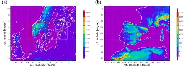
Fig. 1. LM model domains for 7 km, 2.8 km and 1.1 km resolution. (a) Helsinki and Oslo. (b) Valencia.

description of LM model design and physics is given in Step-peler et al. (2003) and in the documentations provided at the COSMO web site (http://www.cosmo-model.org). The LM version LM 3.5 operational at the time of the simulations was used.

The LM is nested by one-way interactive nesting into the DWD’s global model GME with approximately 60 km hori-zontal resolution/31 vertical layers and a 2-layer soil model (Majewski et al., 2002, version gmtri 1.25) at the time of the experiments (while later 40 km/40 layers, a multi-layer soil model and ice phase cloud microphysics were included). The LM is operationally initialised in a four-dimensional data as-similation cycle based on a nudging analysis scheme. Lat-eral boundary values are provided from GME forecasts. The operational one-way nesting procedure is applied with time-dependent relaxation boundary conditions similar to Davies (1976). Using a relaxation boundary zone depth of 8 LM grid points effectively reduces numerical noise created by bound-ary inhomogeneity. The interpolation of initial and lateral boundary data from GME to LM is performed with a model-adapted interpolation scheme.

2.2 The LM set-up and nesting for the episode simulations The target city simulations in FUMAPEX are designed to follow the operational procedures of the participating weather services as closely as possible. As the target cities Helsinki and Valencia are located outside the operational LM area, the LM domain had to be shifted to Scandinavia and the Iberian Peninsula, respectively. The LM 7 km nest area cov-ers a large region of 365×285 grid points (2550×1990 km2)

in order to allow development of mesoscale structures in LM independent of GME, especially on the windward side of the target cities. The Scandinavian area also served as outer nest for the Oslo simulations. For each target city, two further

one-way self-nested LM domains were inserted as shown in Fig. 1. In contrast to other mesoscale models like MM5 and RAMS, the LM allows nesting with any nesting factor, thus a factor of 2.5 was chosen in order to subdue numerical noise. For the experimental 2.8 km and 1.1 km LM nest simulations, no data assimilation and initialisation was performed, but in-terpolated initial conditions and boundary relaxation were applied. The LM seems quite robust towards initial imbal-ances, at least from the experience with the operational ver-sion. The initial and boundary values were interpolated from the outer to the inner LM nests with an LM–adapted inter-polation tool. The medium nest for each target city covered 297×237 grid points (830×660 km2)with 2.8 km horizontal resolution. The number of vertical layers was also increased from 35 to 45, especially in the lower boundary layer, with the centre of the lowest model layer moving from about 33 m to 20 m, and now 13 layers compared to the operational 8 layers in the lowest 1000 m.

The third, inner city nest still encompasses 247×197 grid points (270×200 km2)with 1.1 km horizontal resolution and 45 layers. The chosen nests are comparatively large as the forecast length in all resolutions is 48 h in order to satisfy the requirements of the urban air quality community to take pol-lution abatement action a day in advance. Special care was taken to avoid placing any nest boundaries on high moun-tains like the Pyrenees and the Norwegian mounmoun-tains north of Oslo in order to avoid creating numerical noise or model instability.

Three of the six episodes considered are dated before Dec 1999 when GME analyses are not readily available. A GME cold start was performed using one ECMWF ERA-40 analy-sis per episode and running the GME for 8 days before start-ing the episode simulations in order to extstart-inguish ECMWF model influence on the GME as far as possible. The remain-ing episodes were re-run from one archived GME analysis

while the lateral boundary values during the forecast were again derived from the corresponding GME forecasts, not from analyses to keep in line with the quasi-operational fore-cast mode of the experiment.

A new set of physiographic parameters was derived for all grid points of each of the 8 LM domains using the same procedure and database as for the operational LM.

2.3 Meteorological description of target city episodes The project target cities and episodes were chosen from the cities active or interested in air pollution abatement strate-gies. They represent a variety of European climate regions, seasons and topographic conditions which determine the rel-ative importance of meteorological and other factors caus-ing the episodes (Valkama and Kukkonen, 2004). Explic-itly long-range transport episodes were excluded from this study in order to focus on local and mesoscale meteorologi-cal phenomena in the high-resolution simulations. The cities involved include Helsinki as a Northern European city with almost flat topography situated on a broken coastline. Oslo is located on an inland fjord enclosed on three sides by hills forming a basin. The Valencia/Castell´on area is a conurba-tion on the flat, open Iberian coast neighbouring high moun-tains up to 2000 m and with long, deep valleys reaching in-land.

The episodes represent typical regional variants. The Helsinki episodes are winter inversion-induced and spring dust episodes involving particles (and nitrogen dioxide) with possible suspension of particles after thaw and include an extreme radiation-induced inversion case for 1995 (Kukko-nen et al., 2005). The Oslo episodes are also typical win-ter inversion and particle suspension episodes (involving ni-trogen dioxide) where inversion conditions are enhanced by topographical mountain basin effects (Valkama and Kukko-nen, 2004). The characteristic episode in the Iberian coastal mountain region is a photochemical episode including ozone and particles in spring and summer and depends on complex mesoscale recirculation of pollutants and longer recharging periods (Mill´an et al., 2002). All episodes can last for one week or more but for the simulations only forecasts cover-ing the most characteristic 3 days (in winter, 5 in summer) were chosen. The episode characteristics following the clas-sification in Kukkonen et al. (2005) are described in Table 1. Additional episode information is provided in the individual target city chapters.

3 Results and evaluation

3.1 Model evaluation

The evaluation focuses on the meteorological parameters rel-evant in the urban environment and performed against mea-surements at urban observation stations whenever possible. The different climate regions, seasons of the year and episode

types require a different focus of evaluation for each tar-get city (Sokhi et al., 2002; Piringer and Kukkonen, 2002; Kukkonen et al., 2005). The LM performance in forecasting the main meteorological factors characterising the episodes is evaluated using horizontal fields and vertical profiles for single parameters at station locations every 6 forecast hours, 48 h forecast time series of single parameters and of vertical profiles at station locations and vertical cross-sections.

The model forecasting skill at fixed observation stations also depends on the quality and representativeness of these observations. The observations of the mainly WMO SYNOP stations considered passed the standard QA checks. The representativeness of the station location and set-up espe-cially in cities (often on roof buildings), however, is often poor (Piringer et al., 2005). Measurements are thus assumed to represent 2 m temperature and 10 m winds without any height corrections. In the LM, the corresponding 2 m tem-perature and 10 m winds are derived diagnostically from sur-face and lowest model layer values in the constant flux layer using improved stability functions which are neither derived from Monin-Obukhov similarity theory nor measurements but from the LM turbulence closure (Mellor and Yamada, 1974). Some meteorological parameters are also modelled as instantaneous values while the measurements are reported as time averages (like wind speed and direction, reported as 10 min or hourly averages). Additionally, representativeness is influenced by the largely diverging volumes for the sta-tion observasta-tions and the model grid boxes which also differ by a factor of about 70 for the lowest grid box between the LM with 7 and 1.1 km resolution. With increasing model resolution and detail of the simulations, traditional verifica-tion approaches at fixed staverifica-tions are degraded (compared to larger scale forecasts and despite improved mesoscale struc-tures) by model time and space errors and deficiencies of the observing network, e.g. data scarcity and representativeness problems (Mass et al., 2002, see also for a comprehensive discussion of mesoscale model predictability). The opera-tional 7 km LM forecast equations and results are evaluated in the daily NWP process while the higher resolution sim-ulations must remain inadequate due to known deficiencies of not yet scale-adapted and non-urbanised physiographic parameters and physical parameterisations. Important mi-croscale effects of urban structure (like street canyons) are neither resolved nor yet parameterised in the Lokalmodell.

These aspects cast considerable uncertainty on model val-idation against point measurements. Therefore, deteriora-tion of model evaluadeteriora-tion at stadeteriora-tion locadeteriora-tions with increas-ing model evaluation must not necessarily deny model im-provement. It was thus important to broaden the evaluation by considering the consistent behaviour of the meteorologi-cal fields in space and time for judging model improvements (Skouloudis, 2000; Mass et al., 2002). For these reasons, but also due to the restricted amount of data available for the episodes, statistical scores at observation stations are not presented here. The episode error ranges, however, were

Table 1. Meteorological episode charateristics.

Episode simulation (full episode)

Characterisation

Helsinki

27–29 Dec 1995 – Local winter inversion-induced episode (with high NO2, CO and PM10)

– Extremely strong ground-based inversion (−16◦C in lowest 90 m, −18◦C in 125 m), induced by long-wave radiation

– Persistent stable (even daytime!) to very stable nocturnal stratification

– High pressure, very cold (−25◦to −2◦C) and mainly dry, little cloud, low to moderate west-erly winds, slight snowfall on 28 Dec

– Snow cover, sea ice belt only ca. 11 km broad along coast – Warm front passage on 29 Dec ends episode

Helsinki

22–24 March 1998 (21–31 March 1998)

– Local spring dust episode (suspended particles)

– Nocturnal ground-based inversion (induced by long-wave radiation) – Neutral to very stable (nocturnal) stratification with strong diurnal variation – Very high pressure, −10 to +4◦C, dry, very low south(westerly) winds – Melting snow

Helsinki 9–11 April 2002 (8–13 April 2002)

– Local spring dust episode (suspended particles from sanded streets) – Nocturnal ground-based inversion (induced by long-wave radiation)

– Near-neutral to very stable (nocturnal) stratification with strong diurnal variation – High pressure, very slight southeasterly winds

– Sunny and very dry, cold cloudless nights, large diurnal cycle of T2m – No snow or ice

Oslo

17–19 Nov 2001 (12–22 Nov 2001)

– Local dust episode (suspended particles, high PM10)

– Nocturnal ground-based inversion, intermittent due to periods with stronger surface winds (5–7 m/s) due to northwesterly foehn

– High pressure, dry, cool (0◦to 9◦C) – No snow or ice cover

Oslo 6–8 Jan 2003 (1–11 Jan 2003)

– Inversion induced episode (highest ever Oslo NO₂, high PM_2.5)

– Very strong, locally varying inversion, induced by long-wave radiation and enhanced by warm advection aloft

– High pressure, dry and very cold (−18◦to −2◦C) near ground – Snow and ice cover on ground

Valencia 26–30 Sep 1999 (29 Aug–1 Oct 1999)

– Photochemical pollution episode (ozone)

– Periodic recirculation, development of mesoscale combined sea breeze/upslope wind circula-tions, stable conditions

– High pressure, low isobaric gradient, strong insolation

1

(a)

(b)

(c)

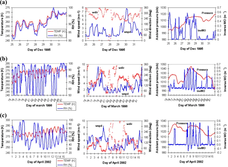
Fig. 2. Meteorological observations (plus FMI-MPP-model-derived inverse Monin-Obukhov number stability index) at Helsinki-Vantaa airport for (a) December 1995, (b) March 1998, (c) April 2002 (from FUMAPEX data web pages of the Finnish Meteorological Institute).

compared to averaged seasonal or one year scores of opera-tional LM 7 km simulations for various urban regions in Fay et al. (2005).

3.2 LM simulations for Helsinki episodes

Especially in northern Europe, ground-based inversions caused by radiation cooling or warm-air advection aloft are the key meteorological factors leading to episodes with often very high levels of pollution. Low wind speeds and stable atmospheric stratification also play an important role in caus-ing low ventilation and air pollution episodes as elsewhere in Europe (Sokhi et al., 2002; Pohjola et al., 2004; Rantam¨aki et al., 2005). Specific site topography (mountains, coast) also has a large influence, and usually high pressure anticyclonic situations prevail.

In Helsinki, episodes occur in winter and spring and par-ticulate matter and nitrogen dioxides are the most impor-tant polluimpor-tants. The episodes investigated are local-scale,

ei-ther inversion-induced or spring suspended particle episodes with nocturnal inversions. The key characteristics are inver-sions, atmospheric stability and low wind speeds (Kukkonen et al., 2005), but cloudiness, humidity, surface heat and radi-ation fluxes, and boundary layer height were also evaluated. The extreme winter inversion episode of December 1995 was due to long-wave radiation cooling of the snow-covered ground. The episode days for the March 1998 and April 2002 episodes are classified as suspended particle episodes. Meteorological observations and a measurement-derived sta-bility index (Pohjola et al., 2004, and FUMAPEX web site of the Finnish Meteorological Institute) at Helsinki-Vantaa airport are illustrated in Fig. 2 for the three episodes. The exceptionally high and persistent stability is apparent in the measurement-derived inverse Monin-Obukhov length for the extreme inversion episode of December 1995.

Before evaluating the simulations the changes in phys-iographic parameters with increasing LM resolution are

1

(a)

(b)

Fig. 3. Vertical profiles of forecast temperature [◦C] for LM 7.0 km, 2.8 km, 1.1 km grid resolution for Kivenlathi mast including observations on 28 December 1995, 00:00 UTC (a) +6 h and (b) +36 h.

Table 2. Change of LM physiographic parameters with increasing LM resolution at Helsinki observation stations (in brackets number of national station). Surface soil type for the grid point nearest station: 3=sand, 4=sandy loam, 6=clayey loam, 9=water.

WMO station

Station name Lat Lon H[m] Surface land cover Surface soil type

(national no.) Fraction of grid point

7.0 km 2.8 km 1.1 km 7.0 km 2.8 km 1.1 km 2988 Isosaari 60.10 25.07 5 0 0 0 9 9 9 2963 Jokioinen 60.82 23.50 103 0.99 1 1 6 6 6 2978 Kaisaniemi 60.17 24.94 4 0.32 0.34 0.84 9 9 3 (0334) Kivenlahti 60.18 24.65 44 0.82 0.95 1 3 3 4 2974 Vantaa 60.32 24.97 56 1 1 1 4 6 6

discussed. For the rather flat Helsinki area, orographic heights remain below 200 m for all resolutions. The influ-ence of higher resolution physiographic parameters for the inner LM nest is most evident in the much more indented coast line. Table 2 lists the changes with increasing resolu-tion in land/sea mask and soil type at the Helsinki observa-tion staobserva-tions. Both are remarkably influenced by grid res-olution caused by an increasing number of LM grid points changing from sea to land points in the direct vicinity of the observation stations. The decimal land cover value reflects the proportional influence of land and sea grid points at the station location. The island of Isosaari is too small to be described as a land point even in the highest resolution of 1.1 km. Kaisaniemi is located near Helsinki harbour, and the land fraction is clearly increasing with resolution. For the surface soil type, the value of the nearest grid point is listed. The changes in Kaisaniemi, Kivenlahti and Vantaa directly influence the soil-dependent physiographic parameters (e.g. heat conductivity, heat capacity, field capacity) and lead to

the changes in e.g. the heat and moisture budget of the model described below (Neunh¨auserer and Fay, 2004).

3.2.1 Evaluation of temperature, inversions, stability and wind fields

The 1995 Helsinki episode is caused by an exceptionally per-sistent, strong and shallow ground-based inversion. The in-version strength amounted to 18◦C in the lowest 125 m for the Jokioinen sounding and 16◦C in 91 m at the Kivenlahti mast on 28 December 1995, 01:00 UTC when the snow-covered ground was cooled extensively by long-wave radi-ation under a clear sky (Rantam¨aki et al., 2005). A similar inversion intensity was not reported previously in other Euro-pean urban areas (Piringer and Kukkonen, 2002). Inversions persisted to a lesser extent even during the daytime until the evening of 29 December when they dissolved under warm front influence. The ability of the model to reproduce these dominating feature is investigated first. Figure 3 shows verti-cal temperature profiles at the Kivenlahti radio tower for LM

1

(a)

(b)

(c)

Fig. 4. Time series of 2 m temperature [◦C] for 48 h LM forecasts for 7.0 km, 2.8 km, 1.1 km resolution starting 28 December 1995, 00:00 UTC, for (a) Vantaa, (b) Kaisaniemi, (c) Isosaari.

at 7.0 km, 2.8 km and 1.1 km grid resolution, compared to station observations. The inversion itself is captured by the model. The inversion strength is underestimated with each of the three grid resolutions for the extreme inversions dur-ing the night of 28 December, reachdur-ing up to +18◦_{C for the}

2 m temperature at Jokioinen and Kaisaniemi. This overpre-diction decreases with increasing model resolution but still exceeds 7◦C in the best case. The less intense daytime inver-sion on 29 December 1995, 12:00 UTC (Fig. 3b), is much better described and even overpredicted in strength for the higher model resolutions.

Figure 4 compares the 2 m temperature results of LM for the 28 December 1995 forecasts to station observations. The large diurnal temperature variation is not simulated in the wintertime episode. Nevertheless, while there is little change due to grid refinement in Vantaa and Isosaari, the Kaisaniemi results move from the sea characteristics of the Isosaari tem-peratures to the inland values at Vantaa with increasing res-olution. The same behaviour is found for sensible and latent heat fluxes. This confirms the positive impact of the increas-ing land fraction on the physiographic parameters for the LM grid points representing Kaisaniemi as shown in Table 2. On the other hand, Isosaari has no diurnal temperature cycle for any LM resolution as it always remains a sea location.

In an attempt to explain the large temperature bias of LM especially for the nocturnal minima during the inversions, several meteorological factors are studied in the following paragraphs.

Large initial forecast errors often stem from model spin-up or data assimilation problems and may contribute to the poor inversion prediction. In the experiment, only 00:00 UTC forecasts are used but the strongest inversions and tempera-ture minima occur around 00:00 UTC for the episode. There is no surface data assimilation of temperature in LM, but soil moisture, sea surface temperature and snow height are ana-lysed at the start of the 00:00 UTC predictions which are used in this study. The short forecast with recent data

assim-ilation and initialisation may even improve slightly for the 2 m temperatures around 00:00 UTC (near-minimum temper-ature) compared to the medium and long forecast of 24 h or 48 h previously. A spin-up error may thus contribute to the deviations but is usually small compared to observed near-surface errors of up to 11◦C.

Cloud cover has a strong influence on long-wave cooling of the surface and is investigated as far as observation records permit. The detected small deficiencies in the forecast of cloud cover and hence the effect on long-wave radiation are likely to contribute only slightly to the overall temperature and inversion error in the December 1995 episode.

A snow cover was observed and is also analysed and fore-casted in LM. Snow height in LM referred to loose powder snow independent of age, density, heat capacity and con-ductivity which may influence surface temperature, vertical fluxes and consequently the development of shallow inver-sions (Rantam¨aki et al., 2005). As the influence of snow treatment in the LM soil scheme on temperature and inver-sion prediction was suspected to be large, an increase of snow density with age and a snow albedo depending on snow age and forest cover are now operational in LM in order to im-prove the thermal effects on the 2 m temperature. Addition-ally, an improved 7 layer soil scheme with freezing and melt-ing of soil water and ice was introduced.

A narrow belt of (mainly new) sea ice of 11 km width was observed on the Gulf of Finland near Helsinki (Ice chart No. 29.12.1995 of Finnish Institute of Marine Research). No ice cover at all was simulated with the LM which uses sea ice information assimilated in the global model GME be-cause the observed ice belt was not detected in the coarse GME assimilation grid, but improvements of sea-ice effects in LM are under development. Rantam¨aki et al. (2005) con-clude from sensitivity studies that the ice cover on the Gulf of Finland may have a substantial effect on surface parame-ters. This atmospheric response may be advected downwind and ashore where the effects on the planetary boundary layer

1

(a)

(b)

(c)

Fig. 5. Vertical profiles of (a) horizontal wind speed [m/s] as 48 h time series at Kivenlathi mast for LM 7.0 km, 2.8 km, 1.1 km grid resolution and observations (top to bottom), (b) wind speed [m/s] for 28 December 1995, +6 h, (c) potential temperature [◦C] for 28 December 1995, 00:00 UTC +6 h.

can be crucial for air quality applications (Drusch, 2005). In LM, the proximity to comparatively warm open water instead of the observed ice cover directly influences meteorological parameters at the coastal grid points. This adds to the neces-sity to investigate wind speed and direction observations and forecasts carefully even in this radiation-induced inversion episode.

The correct simulation of low model wind speeds and suf-ficient atmospheric stability are the further key requirements for correct inversion episode forecasting and are closely con-nected to inversion modelling. Synoptic westerly winds are observed above the inversion together with unusually warm air caused by warm advection and anticyclonic subsidence. Vertical profiles of wind direction show a southerly bias in LM forecasts compared to measurements. The vertical pro-files of horizontal wind speed shown in Figs. 5a–b exhibit a frequent shape especially for the winter episodes with over-estimation of velocity near the surface and underover-estimation aloft. This comparison indicates overpredicted vertical ex-change and insufficient LM stability. The unusually warm air aloft would then be mixed down and contribute to the temperature overprediction near the surface. Evaluation of 10 m winds in Fig. 6 reveals varying performance of 10 m horizontal wind speeds. The pattern of larger wind speed variations is captured, with the forecast improving with in-creasing grid resolution as for 29 December 1995, belong-ing to the warm front passbelong-ing Helsinki and markbelong-ing the end of the episode (Figs. 6b–c). Slight wind velocity values are overpredicted at all stations especially in the strongest inver-sion night of 27 to 28 December and calms are not fore-casted at all (Figs. 6a–c). This again points to insufficient stability for the episode simulations as discussed above. LM vertical profiles of potential temperature, however, demon-strate strong to very strong thermal stability at the inland sta-tions and mainly stable and some neutral stratification at the

coastal stations of Kaisaniemi and Isosaari (Fig. 5c). There is, however, a temporal decrease of stability on 28 Decem-ber, 00:00 UTC, at all stations. On the other hand, for very stable winter episodes, the overestimation of 2 m tempera-tures and 10 m winds may be due to suspected insufficient stability influence on the transfer coefficients and the intro-duction of minimum diffusion coefficients for stable situa-tions in LM causing overestimation of vertical exchange that reduces the overall inversion strength. For strong inversions, 2 m temperature may also be overestimated by specific fea-tures of the stability-dependent interpolation between surface and the lowest prognostic level in the LM (Neunh¨auserer et al., 2004).

The overprediction of very slight wind speeds or a lack of calms may have a great influence in regions of large tem-perature contrasts as between the very cold land mass and the unfrozen sea. Erroneous temperature advection might then seriously change the simulated meteorological and pol-lution conditions of this basically local episode. Forecasts of wind direction must then also be investigated as an addi-tional cause or explanation of the model failure to simulate the inversions.

During the strongest inversion night of 27 to 28 Decem-ber, calms or low winds <2.5 m/s are observed at the sta-tions (with only one exception of 7 m/s at the island station Isosaari on 28 December, 06:00 UTC, presumably due to di-rect sea influence). The lower boundary layer winds were also weak, at least up to the 100 m level for the Kivenlahti mast (Rantam¨aki et al., 2005). These wind speeds are over-predicted with all LM versions. In Vantaa e.g., there is a calm in 10 m winds from 27 December, 18:00 UTC, until 28 De-cember, 03:00 UTC, while the LM with all resolutions simu-lates mainly southwesterly (to southeasterly) winds between 1–2.5 m/s (Figs. 6a, d) which advect comparatively warm and moist sea air from the Baltic (11 km ice belt observed,

1

(a)

(b)

(c)

(d)

(e)

(f)

Fig. 6. Time series of 10 m horizontal wind fields for 48 h LM forecasts for 7.0 km, 2.8 km, 1.1 km resolution starting 28 December 1995, 00:00 UTC, top: wind speed [m/s] for (a) Vantaa, (b) Kaisaniemi, (c) Isosaari, and bottom: wind direction for (d) Vantaa, (e) Kaisaniemi, (f) Isosaari.

with no ice in LM) in the nocturnal hours around the inver-sion maximum (Fig. 4a) when the 2 m temperature is over-predicted by 10◦to 12◦C in the LM versions. Very similar situations prevail at Kaisaniemi (Figs. 6b, e) and Kivenlahti stations. At the harbour station Kaisaniemi with the largest 2 m temperature errors of +14◦C to +18◦C, the forecast may additionally deteriorate due to the immediate coastal situa-tion at the open ice-free LM Baltic instead of the sea ice belt in combination with reduced stability and additional over-prediction of vertical exchange, wind speed and warm ad-vection. The neighbouring grid points also partly remain sea points with incorrect physiographic parameters (see Table 2). The simulated temperature development at all stations seems sensitive to the combined error in wind speed and northerly or southerly deviations from observed winds and, correspondingly, insensitive even to large errors of wind speed as long as the wind direction is correctly simulated. The missing diurnal cycle of temperature and nocturnal tem-perature minimum in all LM station forecasts from 28 De-cember, 00:00 UTC, corresponds to underpredicted stability and overpredicted vertical exchange and wind speeds com-bined with wind directions in favour of the southwesterly, i.e. seaward direction from the basically unfrozen Gulfs of Finland and Bothnia. Even the island station Isosaari, which

is a LM sea grid point, shows this dependency although to a lesser extent (Figs. 6c, f).

In conclusion, the large nocturnal errors of LM forecasts of near-surface temperatures and inversions experienced es-pecially on 28 December may be caused by a whole range of factors that interact in a highly non-linear way and partly intensify. These include insufficient stability influence on transfer and diffusion coefficients, overestimated vertical ex-change and mixing- down of warm air from aloft, reduction of strong stability, erroneous lower level warm advection due to errors in wind speed and direction in an area of large tem-perature contrasts, lack of sea ice for the episode, and de-ficiencies in the snow treatment in the LM soil scheme and partly in physiographic parameters as well.

As Helsinki is positioned outside the operational LM do-main, no long-term performance scores are available. Over-prediction of 2 m temperature of >10◦_{C is far beyond the}

2◦C bias that is considered satisfactory for the typical LM temperature forecast. The December 1995 Helsinki episode is thus certainly not only the most extreme inversion episode observed in southern Finland but also an extreme case of poor model performance for the LM. Poor performance is reported for other NWP models like MM5, HIRLAM and RAMS (Berge et al., 2002; Pohjola et al., 2004; Fay et al., 2004;

1

(a)

(b)

(c)

(d)

(e)

Fig. 7. LM 48 h forecasts for 7.0 km, 2.8 km, 1.1 km resolution starting 23 March 1998, 00:00 UTC, and observations. Top: Vertical profiles as 48 h time series for (a) temperature [◦C] and (b) relative humidity [%] (top to bottom: 7.0 km, 2.8 km, 1.1 km, observations). Bottom: 48 h time series of 2 m temperature [◦C] for (c) Vantaa, (d) Kaisaniemi, (e) Isosaari.

Rantam¨aki et al., 2005) for this strong inversion episode as well.

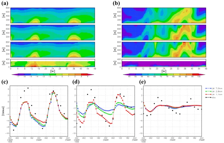
In both spring episodes, the observed ground inversions are still stronger at night with inversion strengths of up to 8◦C but lift and disappear during the day. Exemplary vertical profiles for 23 March 1998 in Fig. 7a show that the largest temperature errors are now found in the upper part of the inversion layer, not near the surface, but are reduced to be-low 5◦C. Temperatures are generally underpredicted in the whole lower troposphere from the ground upwards, except in some nocturnal inversions. Additionally, the amplitude of the diurnal temperature cycle especially at the ground, but also aloft is generally underpredicted. This points to the typical springtime LM tendency of premature thaw and exceeding soil moisture in the upper soil level leading to exceeding la-tent heat fluxes, overpredicted relative humidity in the lower boundary (Fig. 7b) and underpredicted temperatures.

The less extreme spring episodes, nevertheless, show im-proved near-surface temperature forecasts for all LM resolu-tions with deviaresolu-tions mainly below 4◦C even in the noctur-nal inversions. The diurnoctur-nal variation of the 2 m temperature

is well developed at inland stations in spring (Fig. 7c) but maxima are often underpredicted due to the exceeding upper soil moisture. Only at the island station Isosaari the ampli-tude of the diurnal cycle remains underpredicted because the station is a sea grid point in LM (Fig. 7e). The results at the near-harbour station Kaisaniemi benefit clearly from the growing land fraction and improved physiographic parame-ters as the diurnal cycle is best captured with the highest res-olution (Fig. 7d). Diurnal cycles for sensible and latent heat fluxes are also developed with increasing resolution and land fraction as well. Wind speed forecasts tend towards over-prediction of low wind speeds and underover-prediction of larger ones. Deviations in wind direction may still be large but their influence on temperatures is reduced due to the diminished temperature contrasts in the region in spring.

3.2.2 Evaluation of boundary layer and inversion heights Further key thermodynamic factors for pollutant episodes are atmospheric stability and boundary layer height. Strong stability is predominant especially in northern inversion episodes where strongly stable stratification may persist even

1

(a)

(b)

(c)

Fig. 8. Horizontal fields of boundary layer height [m] calculated with the gradient Richardson number scheme for the 1.1 km LM forecast for 28 December 1995, 00:00 UTC +12 h. (a) daytime mixing height showing mainly undefined values in violet, (b) stable nocturnal scheme without replacement strategy showing mainly undefined values (below 1200 m) in red (c) vertical cross section of turbulent kinetic energy [m2/s2] through Jokioinen (near left margin of figure) and Kivenlahti (near right margin).

during most of the day like for the extreme inversion episode of December 1995 (Fig. 2a). The stability of the PBL char-acterises the dispersion qualities in the boundary layer while PBL height determines the volume available for pollutant dispersion and the resulting concentrations and thus is one of the fundamental parameters in many dispersion models.

At the DWD, the operational gradient Richardson num-ber scheme based on the diagnostic version of the turbulence parameterisation scheme of LM (following Mellor and Ya-mada, 1974, level 2) was evaluated with good results in a wide variety of synoptic situations (Fay et al., 1997). For the extremely strong and shallow inversion-induced 1995 wintertime episode the determination of pollutant-relevant “mixing” heights is difficult. The continuous Kivenlahti mast observations and the Jokioinen soundings show a quasi-permanent ground inversion up to 100–200 m rising to 400– 500 m for Jokioinen soundings at 12:00 UTC on 28 Decem-ber (Rantam¨aki et al., 2005). Strongly stable conditions per-sist almost continuously from 27 December up to the noon of 29 December with the maximum inversion strength during the night of 28 December (Fig. 3a). Thus even during the day, a stability situation typical for the stable nocturnal inversion is retained (Zilitinkevitch et al., 2002). Pollutants are proba-bly trapped to a greater part under this inversion causing the episode. On the other hand, warmer air from advection and subsidence remains aloft. Boundary layer heights derived from LM vertical profiles of potential temperature show in-version heights of between 200 and 300 m for Jokioinen and Kivenlahti. LM potential temperature profiles also describe a decline of the very strong stability above the inversion but with strong stability still found in all higher levels. Deriving boundary layer heights with a turbulent kinetic energy (TKE) depletion approach (using a 5 or 10 per cent depletion crite-rion) on the LM TKE cross section shown in Fig. 8c would lead to more appropriate values rising above 400 m inland near Jokioinen at 12:00 UTC. This contrasts with results of

Baklanov (2000), where stable inversions were largely un-derestimated with the TKE depletion approach for the CPR turbulence scheme and confirms that the approach is also very sensitive to the turbulence scheme.

The Richardson number scheme for the daytime mixing height, however, describes a noon boundary layer height of up to 1200 m mainly along the coast that might belong to a higher “rural” or elevated residual boundary layer on top of the shallow inversion. Mixing heights remain undefined at many grid points (Fig. 8a, violet colour) because the Richard-son number scheme for the synoptic daytime mixing height is based on the detection of the transition between a dynam-ically and thermally unstable layer to a stable one. It is thus unable to describe a boundary layer in stable stratification extending high into the troposphere. Further investigations show that the stable stratification at most undefined points extends above 1000 m (Fig. 8b, red colour) so that the sec-tion for determining stable PBL heights in the mixing height scheme could not be successfully applied, either.

For the 1998 spring episode, the typical diurnal cycle of rising BL height during the near-neutral daytime con-ditions is simulated, with noon or afternoon maxima and a collapse towards the nocturnal stable heights. Mixing heights increase from lower coastal values of 200 m to inland heights of 600–800 m on 24 March and 1000–1200 m on 25 March at 12:00 UTC. They agree with vertical profiles of LM potential temperature and turbulent kinetic energy (TKE depletion approach) and validate well in comparison with Jokioinen radiosoundings and with further mesoscale mod-els in FUMAPEX. The development of the mixing heights is found to be delayed and slightly reduced (100 m) due to overpredicted cloud cover and the effects of premature LM thaw which lead to exceeding moisture in the upper soil level, reduced 2 m temperature, sensible heat flux and mix-ing heights. The mixmix-ing heights for 10 April 2002 show the same overall behaviour but increased maximum heights of

1

(a)

(b)

(c)

(d)

(e)

(f)

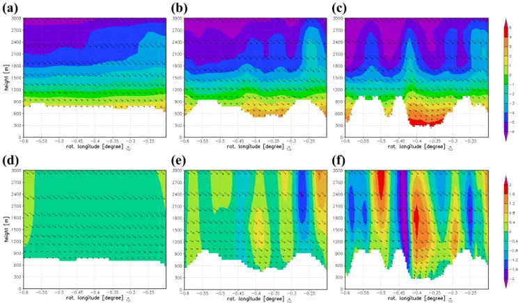
Fig. 9. Oslo forecasts with LM of 7, 2.8, 1.1 km resolution, 17 November 2001, 00:00 UTC +18 h. Vertical cross section along Hallingdal valley with horizontal wind speed and direction (black arrows) and shaded (a–c) temperature [◦C], (d–f) vertical velocity [m/s].

1400–1500 m due to higher temperatures. The comparison with radiosoundings even improves due to the correct fore-cast of cloud cover and absent snow.

The LM gradient Richardson number scheme for mixing heights is thus capable of simulating daytime mixed bound-ary layer heights well for the Helsinki spring episodes with slightly unstable to near-neutral stability. It necessarily fails for the very stable daytime conditions during the December 1995 episode. However, inversion heights derived from ver-tical profiles of LM TKE and potential temperature succeed in simulating observed heights. These results highlight the general problems of simulating boundary layer or inversion heights under stable conditions even in the rural environment (independent of questions of urban mixing heights and inter-nal boundary layers) and the need for improved schemes and model parameterisations especially for stable (not only noc-turnal) conditions (Zilitinkevitch et al., 2002; Piringer and Joffre, 2005).

3.3 LM simulations for Oslo episodes

Episodes in Oslo occur in the winter half-year and are inversion-induced or suspended dust episodes. Therefore, the same key episode parameters apply as to Helsinki, i.e. ground-based inversions, stable atmospheric stratification and low wind speed, but combined with complex

orogra-phy. The surrounding mountains in the shape of a large topo-graphical basin formation worsen the dispersion conditions. The strongest inversions are observed in the valleys due to ra-diative cooling at the surface and often warm advection aloft, and reduced wind speeds due to sheltering in stable inver-sion situations when stagnant air pools form that may last for many days leading to concentration levels like in much larger European cities (Valkama and Kukkonen, 2004; Kukkonen et al., 2005). The major pollutant sources today are connected to domestic consumption (private wood and oil burning) and road traffic (road dust suspension by studded car tyres), less to long-range transport or the scarce industry.

Both Oslo episodes are local-emission episodes and dis-tinguished by local factors (strong ground-based inversions) but also synoptic-scale dynamic features. The November 2001 episode shows intermittent breakdowns due to periods of stronger surface winds of 5–7 m/s related to northwest-erly foehn while the January 2003 ground-based inversion is mainly caused by warm advection aloft creating the strong inversion strengths of up to 20◦C for several days. Scarce cloud cover additionally supports the formation of inversions in both episodes. For the Oslo episodes, therefore, the discus-sion focuses on the skill of the LM at simulating temperature, inversions, wind fields, stability and mountain sheltering of stagnant air pools.

1

(a)

(b)

Fig. 10. Time series of 2 m temperature [◦C] for LM 7.0 km, 2.8 km, 1.1 km and observations, 48 h forecast of 06 January 2003, 00:00 UTC. (a) Blindern, (b) Tryvann.

Table 3. Change of LM topographic height with increasing resolution at Oslo observation stations.

Name Station height Station type Model height H[m]

LM 7.0 km LM 2.8 km LM 1.1 km Blindern 95 Urban (temperature obs in 8 and 25 m) 119 40 43

Valle Hovin 94 Suburban 149 121 92

Tryvann 514 Rural hill 249 285 442

Mountain top – – 1040 1183 1245

Valley – – 741 457 262

Changes of orography with increasing LM resolution are expected to substantially influence simulations in the com-plex setting of Oslo between an inland fjord and nearby hills. They are listed in Table 3 for the three Oslo observation sta-tions and two referential sites on a mountain top and in the Hallingdal valley northwest of Oslo.

All LM topographies describe the medium orography and underestimate the height differences between valleys and mountain tops even in the 1.1 km version. Nevertheless, the increase in horizontal grid resolution leads to a considerable improvement of the model topography. The consequences for the model results are striking, even for the cross sec-tion along the Hallingdal valley which does not include the highest mountains. The vertical temperature distribution in Figs. 9a–c exhibits deeper and warmer valleys and higher and colder mountain tops. Wind fields and streamlines be-come more structured and show more numerous and pro-nounced convergence and divergence lines. The higher and steeper orography induces mountain lee wave structures in the vertical velocity field (Figs. 9d–f). The temperature

lay-ers accordingly assume a wavelike pattern of variable inten-sity which agrees with the northwesterly foehn observed over Oslo. This confirms the improved realism of higher resolu-tion NWP results reported e.g. in Mass et al. (2002).

Topography influences temperature in a similar but less distinct way due to the smoother terrain and the smaller height differences at the meteorological stations in the Oslo city area. Generally, LM time series of 2 m temperature for the city stations show good agreement with observations and only little influence of model resolution for the November 2001 episode with temperatures between 0◦ _{and 9}◦_{C. The}

forecast skill for the more extreme and changeable temper-atures of the January episode (initially very cold down to

−18◦C with subsequent warm advection) is much lower. Ob-served temperature minima during the inversion periods are often overpredicted in the Oslo stations Blindern and Valle Hovin, up to +12◦C mainly during the strong inversion in the night from 6 to 7 January (Fig. 10). These errors are usu-ally reduced with higher LM resolution. For both episodes and all LM resolutions, the diurnal temperature cycle of the

1

(a)

(b)

(c)

(d)

(e)

(f)

Fig. 11. LM simulations with 7, 2.8 and 1.1 km resolution on 6 January 2003, (a) Blindern, time series of vertical temperature [◦C], 48 h forecast starting 00:00 UTC +00 h. Time series of vertical temperature gradient [◦C/m] for (b) Hovin and (c) Tryvann/Blindern. Forecasts for 6 January 2003, 00:00 UTC +24 h, vertical LM profiles and radiosoundings at Blindern for (d) temperature [◦C], (e) horizontal wind speed [m/s], (f) horizontal wind direction.

very cold nights with strong inversions is underpredicted like for the December 1995 Helsinki episode, and again at least partially caused by features in the dynamic modelling dis-cussed below. For the winter months 2003 in Blindern, sta-tistical scores for the operational 7 km LM version are avail-able. They show a negative bias of 2 m temperature of up to

−3◦C in winter, but with least underprediction in the early morning hours (Fay et al., 2005). This contrasts sharply with nocturnal overpredictions of above 10◦C and highlights the uncommon and unusually poor LM performance in tempera-ture forecasting for the January 2003 episode.

The sparse observations of cloudiness for the January 2003 episode indicate overprediction of total cloudiness (a general feature in LM, Sch¨attler and Montani, 2005) especially dur-ing the night which would partially explain the overestimated nocturnal minima in contrast to the Helsinki December 1995 episode.

In Fig. 11, forecasts of the vertical temperature profiles and radiosoundings for Blindern for 6 January 2003 are pre-sented. The predictions above the observed inversions (400 to 600 m) agree remarkably well with the soundings. In con-trast to the Helsinki December 1995 episode, the maximum errors sometimes occur near the ground surface with up to

+9◦C at night, in other synoptic cases higher up in the in-version layer. Inin-versions are simulated with all model reso-lutions but are mostly underpredicted in strength and often elevated instead of ground-based. The forecasts usually de-teriorate with increasing LM resolution while in the Helsinki episodes increased model resolution usually leads to at least minor improvement in the simulated inversions. A charac-teristic pattern emerges when looking at time series of verti-cal temperature profiles (Fig. 11a). Synoptic warm advec-tion mainly between 300 and 1500 m starts on 6 January but seems strong enough in layers between about 300 and 900 m only with the 7 km LM when compared to radiosound-ing profiles. For the higher resolutions, therefore, the upper part of the inversion is not enhanced enough by warm ad-vection and remains too cold while the temperatures below about 300 m are overpredicted. In the lowest model layer below 20 m, temperatures drop rapidly leading to a sharp, non-observed near-surface inversion. A similar behaviour is found during all episode days investigated but there is also one near-perfect inversion forecast for the strong inversion of 7 January 2003 when using the (initialised) analysis of 7 January, 00:00 UTC.

The temperature inversions are further investigated using vertical temperature gradients available from observations. A near-surface gradient is established using measured tem-peratures at 8 m and 25 m above ground at Valle Hovin sta-tion. This is compared to the modelled temperature gradi-ent between the lowest model level above the model orog-raphy at Valle Hovin (roughly 34 m for 7 km resolution and 20 m for 2.8 km and 1.1 km resolution) and the 2 m temper-ature (Fig. 11b). In all cases, inversions are indicated by positive values. The temperature gradient tends to increase with higher vertical resolution for the 2.8 and 1.1 km simu-lations. Compared to the measurements at Valle Hovin, the gradient improves with increasing resolution for the Novem-ber 2001 episode but misses the January 2003 observations which hardly show an inversion for the lowest 25 m.

Another approximate temperature gradient covering the lowest 400 m of the boundary layer is introduced between the 2 m temperatures measured at Tryvann hill and Blindern which are only a few kilometres apart although the Tryvann measurements are not identical with free atmosphere condi-tions. The approximate boundary layer inversion strength be-tween Tryvann and Blindern is underpredicted especially in the strong nocturnal inversion of 6 to 7 January. This may be partly due to the 2 m temperature at Blindern being overes-timated by specific features of the stability-dependent inter-polation between surface and the lowest prognostic level in the LM for very stable conditions. The gradient generally improves with increasing horizontal resolution (Fig. 11c). Obviously, the structure especially of strong inversions like those during the January 2003 episode or the Helsinki De-cember 1995 episode is not correctly captured with the LM.

Deficient inversion forecasts may be accompanied (caused or intensified) by deviations of the simulated wind fields as was already shown for the December 1995 Helsinki inver-sions. The observed persistently low 10 m wind speeds (of 0 to 2 m/s especially for the January episode) at Blindern and Valle Hovin especially in the 1.1 km LM are a key cold pool inversion characteristic in the valleys for both episodes. The simulations improve with increasing resolution especially for January 2003 and are well predicted with the 1.1 km (and 2.8 km) LM except at the end of the 3 day period inves-tigated. Time series of LM vertical profiles of wind show an increase in velocities 12–15 h premature at the valley sta-tions compared with observasta-tions leading to premature verti-cal mixing and the early temperature rise in Fig. 10. The LM profiles show a boundary layer wind regime below 600–900 (1200) m distinct from the northerly synoptic winds above. Boundary layer wind speed is permanently overpredicted in the 7 km LM from noon of 6 January until 9 January lead-ing to exceedlead-ing vertical exchange with the warm air aloft. The sharp temperature drop below the inversion top is thus not simulated and the surface temperatures overestimated in the 7 km LM. The vertical profile of the inversion for the higher resolution simulations, especially in the 1.1 km ver-sion, may be explained with different dependencies in

com-parison with radiosoundings at Blindern for 6 January +24 h in Figs. 11d–f. Above 400 m warm advection seems insuf-ficient in combination with overestimated wind speeds lead-ing to a decrease of inversion strength from the inversion top. Below 400 m, the winds are very slight (between 1 and 3 m/s for 1.1 km LM) and underpredicted and turn anti-clockwise to southerly/southwesterly directions with increasing resolu-tion and decreasing height. This may be caused by the higher and steeper model topography leading to lower level stream-lines being diverted around the hills in the deeper valleys and a mountain blocking effect with subsidence penetrating be-low 400 m in LM at the forecast time discussed. The di-verted slight southwesterly winds below 400 m may also lead to warm advection in the air lingering for some hours above Oslo fjord which is ice-free and about 10◦C warmer than the surroundings at the beginning of the night. This agrees with vertical profiles of potential temperature showing that the stratification always remains stable but often with reduced stability in the lowest 200 m for the higher resolutions.

Several effects may thus combine to lead to temperature overprediction and reduced stability in the lower boundary layer above Oslo especially in the 1.1 km version of LM. A similar pattern is encountered during most of the episode and leads to a lifting of the ground-based inversion or even its complete dissolution for the 1.1 km LM versions whereas in the operational 7 km version, inversions remain ground-based and retain a larger inversion strength. For the topogra-phy height and steepness increasing with LM resolution near to the Oslo stations, the decreasing model skill may partly be due to the terrain-following vertical coordinate system that was shown to deteriorate valley inversions close to mountains in comparison with simulations with a z-coordinate model (Steppeler, 2002).

The November 2001 episode is also influenced by a de-cisive dynamic feature. The strong surface inversions break down due to intermittent wind peaks related to northwest-erly foehn penetrating into the Oslo valley basin (Valkama and Kukkonen, 2004). The low wind speeds, but also the observed occurrence and phase of the narrow wind peak are very well represented with the 1.1 km LM (though with underpredicted wind maximum) in Blindern early on 19 November 2001. The LM, however, does not simulate the very sharp Valle Hovin peak late on 19 November 2001 that marks the end of the maximum NOxand particle

concentra-tions at all Oslo air quality staconcentra-tions for the whole episode. In conclusion, the dependencies of meteorological param-eters in the Oslo January 2003 episode are highly complex and seem mainly induced by the changes of topography with increasing LM resolution which may lead to large dynamic and thermal differences between the LM versions themselves and in comparison with observations. In the very-high res-olution LM, not only mesoscale phenomena like gravity waves, channelling and convergence and divergence lines are better developed because of the improved model orography. This version is also capable of differentiating and simulating

local effects like mountain blocking and lee subsidence due to small mountains. In the Oslo January 2003 episode, these improved capabilities still lead to deterioration, which may be due to the specific episode conditions like direction and strength of synoptic flow in relation to the high-resolution model topography in windward of Oslo during that episode and the chance of advected air masses traversing Oslo fjord at a time of high temperature contrasts.

Thus, the main characteristic of winter inversion-induced episodes, i.e. sufficient inversion strength, is not modelled well with all LM resolutions but especially the higher ones for the January 2003 episode. On the contrary, the key factor of low wind speed improves with higher LM resolution thus retaining the slight winds in the lower boundary layer for a longer time and showing the sheltering capabilities of the high-resolution LM.

Comparison with longer-term statistics reveal that the Jan-uary 2003 episode certainly displays extreme meteorological conditions especially concerning inversion strength. The LM during the less meteorologically extreme November 2001 episode thus shows a much improved and satisfactory fore-casting performance.

3.4 LM simulations for Valencia episodes

In Southern Europe, photochemical episodes occur in larger, partly non-urban areas from spring to autumn, often in com-bination with higher particle concentrations and in addition to winter traffic-induced particle episodes. These photo-chemical episodes arise under anticyclonic conditions with low winds and high solar insolation. Recurring diurnal tem-perature cycles play a leading role especially in ozone forma-tion. Additionally, in topographically complex subtropical latitudes like the Mediterranean basin, the appropriate sim-ulation of the non-local mesoscale circsim-ulations is paramount as they govern the distribution of ozone and its precursors (Mill´an et al., 2002).

The modelling domain for the Valencia/Castell´on episode is centered on the Castell´on conurbation with a variety of in-dustries and pollutant emissions. The atmospheric dynamics in the area is governed by the sea and the nearby mountains. The numerous river valleys rectangular to the coast channel the sea breeze and coastal air loaded with emissions towards inland areas where it combines with inland orographic up-slope winds. Mesoscale, non-local effects like orographic injection, return flows and compensatory coastal subsidence lead to recirculation of pollutants and determine the high ozone levels in the whole circulation region at urban scales but may influence synoptic features as well. The interaction between the different scales must, therefore, be reproduced correctly in the models. In contrast to the winter episodes discussed above, these photochemical episodes are frequent or even chronic and are not characterised by meteorological extremes. A full description of the meteorological and air

quality conditions and of simulations is provided in Mill´an et al. (2002).

In this paper, however, only the key episode factor of mesoscale circulations driving pollutant dispersion will be discussed which are the complex mesoscale wind systems and pollutant recirculation.

For the Valencia area, increasing LM resolution involves distinct changes in topographic height and roughness length. The surface roughness decreases at high mountain stations because part of the subscale effects of roughness are assumed to be explicitly taken account of by the parameterisations in the higher resolution LM. The more detailed topography with higher mountains and deeper valleys increases the complex-ity of the temperature and wind fields and improves the de-scription of diurnal breeze circulations, nocturnal drainage winds, coastal subsidence, and of convergence and diver-gence lines, again confirming results for other models (see Mass et al., 2002). In combination with the dynamical and thermal effects due to the changed physiographic parameters, the near-surface fields of temperature, wind speed and direc-tion generally improve with higher LM resoludirec-tion compared to observations.

The evolution of the characteristic mesoscale circulation is discussed in detail in a time series of vertical cross sections and horizontal fields. The vertical cross section in Fig. 12 cuts from the sea to the first high mountain ridge south of the Ebro delta for the forecast starting 27 September 1999, 00:00 UTC. Nocturnal cooling of the high mountains has led to nocturnal drainage winds observed at 00:00 UTC +03 h (05:00 a.m. local time) with boundary layer subsidence in a broad coastal belt (Fig. 12a). At 00:00 UTC +10 h, a sea breeze circulation has developed confined to 800 m depth, as well as an upslope orographic wind further inland and up-hill (Fig. 12b). Both systems are still separated by a nar-row downdraft region possibly enhanced from the mountain gravity wave system aloft. By 00:00 UTC +13 h, both wind systems have combined (Fig. 12c) and their leading edge reaches far inland and even up to the crest of the main moun-tain ridge where they act as a separate orographic chimney for the injection of pollutants aloft. These features fully correspond to observations and description of the circula-tion patterns in Mill´an et al. (2002). The vertical extent of the circulation has risen to about 1300 m. The upper circu-lation branch returns to the coast aloft. The compensatory subsidence along the return leads to subsidence inversions which separate the inland surface breeze from the return flows aloft (Fig. 12c). It also stratifies injected pollutants and creates new (ozone) reservoir layers moving towards the sea where they are mixed down and reinjected into the cir-culation with the sea breeze of the following days. Thus, the high-resolution LM simulates the typical patterns that lead to injection and recirculation of pollutants and to the observed ozone and precursor levels reaching higher values day after day.

1

(a)

(b)

(c)

(d)

(e)

(f)

(g)

Fig. 12. Vertical cross section prependicular to Mediterranean coast north of Valencia (height [m] vs. LM rotated geographical longitude [◦]) for vertical velocity [m/s] (shaded contours) and horizontal wind vector (arrows) for 1.1 km LM forecasts, (a) 27 September 1999, 00:00 UTC +3 h, (b) 27 September 1999, 00:00 UTC +10 h, (c) 27 September 1999, 00:00 UTC +13 h, (d) 28 September 1999, 00:00 UTC +10 h, (e) 28 September 1999, 00:00 UTC +13 h, (f) 28 September 1999, 00:00 UTC +14 h, (g) 30 September 1999, 00:00 UTC +14 h.

1

(a)

(b)

(c)

(d)

Fig. 13. 1.1 km LM streamlines of 10 m wind speed on topographic map of Valencia coastal region with 7 regional observation stations (black dots), coastline in white, axes: LM rotated latitude and longitude [◦]. (a) 28 September 1999, 00:00 UTC +10 h, (b) 28 September 1999, 00:00 UTC +14 h, (c) 28 September 1999, 00:00 UTC +23 h, (d) 30 September 1999, 00:00 UTC +13 h.

These mesoscale circulations change in shape and strength during the five episode days investigated. During the episode with westerly synoptic flow, mesoscale return flow and syn-optic flow reinforce each other. On 28 September e.g., the dominant synoptic scale west winds and strong lee wave pat-tern in the free atmosphere suppress the sea breeze in the morning (Fig. 12d). A small coastal circulation is formed late at 00:00 UTC +13 h showing a closed vertical and also horizontal circulation (Fig. 12e). It grows in size in the af-ternoon but the leading edge only reaches higher mountains after 14:00 UTC that day (Fig. 12f). The recharging period

associated with the periodic sea breeze development in the area is terminated on 30 September 1999 by a cold front pas-sage from the northwest and leads to temporarily decreas-ing concentrations. Coastal stations may experience a short sea breeze development due to the large Mediterranean in-solation and the specific topographic features of this area even under these advective conditions with dominant synop-tic forcing. This regional feature is also simulated with LM (Figs. 12g, 13d).

Figures 13a–b show the period of merging in a time se-ries of horizontal wind fields in the northeastern part of the