An Operational Account of Call-By-Value Minimal and Classical $\lambda$-calculus in ''Natural Deduction'' Form

HAL Id: inria-00389903

https://hal.inria.fr/inria-00389903

Submitted on 30 May 2009

HAL is a multi-disciplinary open access

archive for the deposit and dissemination of

sci-entific research documents, whether they are

pub-lished or not. The documents may come from

teaching and research institutions in France or

abroad, or from public or private research centers.

L’archive ouverte pluridisciplinaire HAL, est

destinée au dépôt et à la diffusion de documents

scientifiques de niveau recherche, publiés ou non,

émanant des établissements d’enseignement et de

recherche français ou étrangers, des laboratoires

publics ou privés.

An Operational Account of Call-By-Value Minimal and

Classical λ-calculus in ”Natural Deduction” Form

Hugo Herbelin, Stéphane Zimmermann

To cite this version:

Hugo Herbelin, Stéphane Zimmermann. An Operational Account of Call-By-Value Minimal and

Classical λ-calculus in ”Natural Deduction” Form. TLCA 2009 - 9th International Conference on

Typed Lambda-Calculi and Applications, Mauricio Ayala Rincón, Jul 2009, Brasilia, Brazil.

pp.142-156, �10.1007/978-3-642-02273-9_12�. �inria-00389903�

An Operational Account of Call-By-Value

Minimal and Classical λ-calculus in “Natural

Deduction” Form

Hugo Herbelin1 _{and Stéphane Zimmermann}2

1 _{INRIA, France}

2 _{PPS, University Paris 7, France}

Abstract. We give a decomposition of the equational theory of call-by-value λ-calculus into a confluent rewrite system made of three indepen-dent subsystems that refines Moggi’s computational calculus:

– the purely operational system essentially contains Plotkin’s βv rule

and is necessary and sufficient for the evaluation of closed terms; – the structural system contains commutation rules that are necessary

and sufficient for the reduction of all “computational” redexes of a term, in a sense that we define;

– the observational system contains rules that have no proper compu-tational content but are necessary to characterize the valid observa-tional equations on finite normal forms.

We extend this analysis to the case of λ-calculus with control and pro-vide with the first presentation as a confluent rewrite system of Sabry-Felleisen and Hofmann’s equational theory of λ-calculus with control. Incidentally, we give an alternative definition of standardization in call-by-value λ-calculus that, unlike Plotkin’s original definition, prolongs weak head reduction in an unambiguous way.

Introduction

The study of call-by-value evaluation in the context of λ-calculus goes back to Plotkin [1] who introduced and studied rules βv and ηv and a

continuation-passing-style (cps) semantics of a call-by-value λ-calculus, named λv. Significant

contributions were made first by Moggi [2] then by Sabry and Felleisen [3] who provided axiomatizations of call-by-value λ-calculus shown by the last authors to be complete with respect to Plotkin’s cps semantics. In the same paper, Sabry and Felleisen also give a sound and complete axiomatization of call-by-value λ-calculus with control (hereafter referred as classical call-by-value λ-calculus). Independently, Hofmann [4] gave an alternative axiomatization of the classical call-by-value λ-calculus.

The theory of call-by-value λ-calculus turns out to be de facto more complex to describe than the one of call-by-name λ-calculus. While β-reduction is enough to evaluate terms in call-by-name λ-calculus and η is enough to characterize the observational equality on finite normal forms (what Böhm separability theorem

expresses, see [5] for a generic account of Böhm theorem vs observational com-pleteness), the situation is more intricate in the call-by-value λ-calculus, where, facing the two rules of the equational theory of call-by-name λ-calculus, the equa-tional theories of call-by-value λ-calculus of Sabry and Felleisen and of Moggi rely on about a half dozen rules3

.

Though, when we observe call-by-name and call-by-value in the context of se-quent calculus [6, 7], the complexity of the respective theories is about the same. Then, what is so specific to natural deduction (of which the standard λ-calculus is a notation for proofs along the Curry-Howard correspondence) that makes call-by-value more complicated there? Let us first give a more precise look at what happens in sequent calculus.

Call-by-name and call-by-value in sequent calculus

In a previous work of the first author with Curien [6], an interpretation of (a variant of) Gentzen’s sequent calculus [8] as a variant of λ-calculus called λµ˜µ-calculus was given, where µ refers to Parigot’s control operator [9]. In this interpretation, the left/right symmetry of sequent calculus pervades into a per-fect syntactic duality first between terms and evaluation contexts, and secondly between call-by-name and call-by-value reduction. Especially, the operator ˜µ, dual to µ, builds an evaluation context that binds the term to which it is ap-plied, as in let x = [ ] in M , in the same way as Parigot’s µ builds a term that binds the evaluation context to which it is applied.

The analysis of λ-calculus through sequent calculus given in [7], whether we consider call-by-name or call-by-value, shows a clear separation between opera-tional rules and observation rules (the operaopera-tional rules are cut-elimination rules and they divide into logical rules that contract the interaction of term construc-tors and evaluation context construcconstruc-tors into more elementary interactions, and two structural rules, one called (µ) for the contraction of µ and one called (˜µ) for the contraction of ˜µ, that duplicate or erase information, moving terms around to possibly create new logical interactions).

A noticeable peculiarity of sequent calculus is that even in the intuitionistic case, the µ operator is required and when sequent calculus is compared to intu-itionistic natural deduction, it turns out that (µ) acts as a commutative cut. What is the problem with call-by-value λ-calculus in natural deduction syntax?

Call-by-value λ-calculus precisely needs commutative cuts so as to reveal redexes hidden by β redexes that are not βv redexes. Take as an example the

term ((λx.λy.y)(zt))u with z, t and u as free variables. With respect to λv, this

term is a normal form, however the reduction between λy and u is possible if

3

The theory of Moggi has seven rules; the theory of Sabry and Felleisen has six axioms of which βlift : E[let x = N in M ] → let x = N in E[M ] is redundant; we will

see later on that isolating βlift out is however important from an operational point

one takes a parallel syntax, like proof-nets or parallel application to obtain the term (λx.u)(zt).

This is due to the presence of free variables, that can hide potential reduc-tions. When using a parallel syntax, one does not rely anymore on syntactical shapes, but on calculus dependencies. In our example, the reduction between λx and (zt) is independent from the reduction between λy and u.

This is where the structural rules announced in the abstract come in: they will denote implicit use of the reduction rule for µ. For call-by-name, we have the well-known σ-equivalence [10] that disentangle redexes, but we have to be more careful for call-by-value. So here, the rule ((λx.λy.M )N )P −→ (λy.(λx.M )N )Pσ is not valid, because one changes the evaluation order of N and P and will break confluence in presence of a µ operator. Our structural rules should then preserve head reduction order to avoid such problems.

1

Call-by-value λ-calculus (λ

-calculus)

In this section, we show how the equational theory of call-by-value λ-calculus can be decomposed into three independent subsystems of rules. Note that we consider here only left-to-right call-by-value.

1.1 The splitting of the usual βv rule

To be able to use what sequent calculus teaches us, we need a construction corresponding to the ˜µ of λµ˜µ. We extend the λ-calculus grammar with a let construction, as follows:

V ::= x | λx.M

T ::= M N | let x = M in N M, N::= V | T

The direct counterpart of this splitting is syntactically expressed by the two following rules:

(⇒) (λx.M )N → let x = N in M (letv) let x = V in M → M [x ← V ]

To understand the intuition behind this, it is necessary to look at how head reduction is performed on an application. We have to check first if M is a value or not, and then if N is a value or not to determine what to reduce. So control is not clear on an application, sometimes it is the left term that has it and sometimes it is the right one.

Using the let is an elegant way to get rid of this. You only need to look at the left term of an application, and when this term is eventually reduced to a λ, it naturally gives the control to the term of the right thanks to the (⇒) rule.

Thanks to this decomposition, we can now have a clear notion of control, and be able to determine where to work on. An evaluation context F is now either an application with a hole on the left, or a hole inside a let, say:

and the mechanism of giving control to the “right” part of the application is now explicit. As we will see later, this will help to solve a standardization problem that arises from this ambiguity.

1.2 Dealing with the implicit (µ) rules

Whenever in the calculus there exists a conditional rule (W )L → R, we will call a pseudo-redex a term matching L but not satisfying the side condition. For call-by-value λ-calculus, the term (λx.x)(yz) is a pseudo-redex, because yz is not a value.

In our calculus, the pseudo-redexes are not of the shape (λx.M )T , but more like let x = T in M . Still, they can hide reductions. Take for example the term (let x = zt in λy.y)u, the counterpart to the term ((λx.λy.y)(zt))u. The reduction between λy and u is still hidden, and we need to get the u inside the let, in a sense. This can be done using the two rules (letlet) and (letapp).

(letlet) let x = (let y = M in N ) in P

→ let y = M in let x = N in P (letapp) (let x = M in N )P

→ let x = M in N P

The (letapp) rule is here to deal with a pseudo-redex on the left side of an

application. If you have a pseudo-redex inside on the left of an application, you can get it outside the application without disturbing the evaluation order, and recover the possible interactions that are independent of the substitution. Using this rule on the example above, we get (let x = zt in λy.y)u → let x = ztin (λy.y)u. The subterm zt still has control during the reduction, but we can do the other reductions as well.

The (letlet) rule has the same role, only for the right part of an application.

1.3 Basic properties of the calculus

Our presentation of call-by-value λ-calculus, called λCBV-calculus, is given in

Figure 1. The auxiliary definition of evaluation context F (resp. E) is used to find the sub-term locally (resp. globally) in control in the term.

The (⇒) and (letv) rules correspond to the (βv) rule, and the (letlet) and

(letapp) rules are the two rules managing the implicit (µ) reductions.

Regarding notations, we will use as a convention that parentheses on the left of an application are implicit, meaning that the term M N P stands for ((M N )P ). In the term λx.M , we will say that the occurrence of x in M are bound and by free variables, we mean variables that are not bound. The set of the free variables of a term M will be written F V (M ).

To avoid problems of capturing variables, we will work modulo α-conversion, i.e. modulo the renaming of bound variables. Therefore, the names for free vari-ables and bound varivari-ables in a given term can always be made distinct. By M[x ← V ], we mean the capture-free substitution of every occurrence of the free variable x of M by V .

Syntax V ::= x | λx.M F ::= [ ]M | let x = [ ] in M M, N, P ::= V | M N | let x = M in N E::= [ ] | xE | F [E] Operational rules (⇒) (λx.N )M → let x = M in Nr (letv) letx= V in N r → N [x ← V ] Structural rules (letlet) let z = (let x = M in N ) in P

r

→ let x = M in (let z = N in P ) (letapp) (let x = M in N )P

r → let x = M in N P Observational rules (η⇒) λx.(yx) r → y (ηE

let) letx= M in E[x]

r

→ E[M ] if x 6∈ F V (E) (letvar) z(let x = M in N )

r

→ let x = M in zN

Fig. 1.The full λCBV-calculus

We write → for the compatible closure of→ and →r ∗

for the reflexive and transitive closure of → . We write = for the equational theory associated. Proposition 1 (Confluence). The operational subsystem, its extension with

structural rules and the full system of reduction rules are all confluent in λCBV -calculus. Otherwise said, for each of these three systems, if M →∗

N and

M →∗

N′

, then there exists P such that N →∗

P and N′

→∗

P.

Proof (Indication). This statement is proved using Tait – Martin-Löf method, applied to the parallel reduction ⇛ defined by the union (of generalizations) of the above reduction rules and the following congruence:

– t ⇛ t – if M ⇛ M′ then λx.M ⇛ λx.M′ – if M ⇛ M′ and N ⇛ N′ then M N ⇛ M′ N′

and let x = M in N ⇛ let x = M′

in N′

Note that (letvar) is redundant in the equational theory but necessary in the

reduction theory to get the confluence.

We say that a reduction relation → is operationally complete if whenever a closed M is not a value, it is reducible along → . For instance, usual β-reduction is operationally complete for call-by-name λ-calculus.

Proposition 2. λCBV equipped with the rules (⇒) and (letv) is operationally complete.

Proof. Any closed term which is not a value has either the form E[let x = λy.M in N ] in which case (letv) is applicable or E[(λx.M )N ] in which case (⇒)

is applicable.

Remark. For simplicity of the definition of λCBV, we did not consider a minimal

set of operational rules. A minimal operationally complete set can be obtained by restricting both M in (⇒) and V in (letv) to be of the form λy.P . However, this

would force to explicitly add an observational rule let x = y in N → N [x ← y]r and a structural rule (λx.N )(E[yM ])→ let x = E[yM ] in N (where the notionr of pseudo-redex and erasing rule, see below, is extended to the case of β-redexes). Associated to reduction rules with constraint, we can define erasing rules used to erase the pseudo-redex part of the rule. Namely, we will use the system composed of the following rule for this:

let x = N in M −→ Ner

A term M is normal for a reduction → if it is not reducible for → . It is structurally normal if, for all N such that M −→er ∗ N, N is normal for the reduction generated by the operational rules. A reduction relation → is

structurally complete if all terms normal for → are structurally normal.

Proposition 3. The set of terms that are normal with respect to the operational

and structural rules is described by the entry Q of the following grammar:

Q::= λx.Q | S | let x = S in Q S ::= x | SQ

Moreover, the reduction generated by the operational and structural rules of

λCBV-calculus is structurally complete.

Proof (Indication). The two parts are proved by induction quite directly. It is interesting to see that in a normal form like let x = P in Q, the leftmost subterm of P is always a free variable and the evaluation of P is blocked by this variable. This suggests an alternative definition of structural completeness based on the notion of evaluation of open terms: a set of rules is structurally complete iff any term which is neither a value nor of the form xM1...Mn or

let y = xM1...Mnin N is reducible.

Let us now focus on the observational rules of Figure 1. Given a confluent reduction → , we say that an equation M = N between normal terms belongs

to the observational closure of → if for every closed evaluation context E and

every substitution ρ of the free variables of M and N by closed values, E[ρ(M )] converges along →∗

iff E[ρ(N )] converges.

Proposition 4. The observational rules from Figure 1 belong to the

observa-tional closure of the set of operaobserva-tional and structural rules of λCBV-calculus.

Proof. When instantiated by closed values, both sides of (η⇒) and (letvar)

con-verge by respectively using (⇒) and (letv), (⇒) and (letlet). For (ηElet), the result

follows by standardization (see below) since at some point, for ρ a substitution of the free variables of E′

[yM ], the reduction of ρ(E′

[yM ]) eventually yields a value and (letv) is applicable.

1.4 The subformula property and structural completeness

The λCBV-calculus can be typed by natural deduction just like the conventional

(call-by-name) λ-calculus. The only new construction is the let, which can be typed by the cut rule. The whole typing system is the following:

Γ, x: A ⊢ x : A Γ, x: A ⊢ M : B Γ ⊢ λx.M : A ⇒ B Γ ⊢ M : A ⇒ B Γ ⊢ N : A Γ ⊢ M N : B Γ, x: A ⊢ M : B Γ ⊢ N : A Γ ⊢ let x = N in M : B

Contrary to the call-by-name λ-calculus, the original call-by value λ-calculus does not satisfy the subformula property for its normal forms. We can distinguish two kinds of “breaking” of this property.

The first one happens with the pseudo-redexes. The term (λx.x)(yz) is a normal form, which can be typed this way, with Γ = y : B ⇒ A, z : B :

Γ ⊢ λx.x : A ⇒ A Γ ⊢ yz : A Γ ⊢ (λx.x)(yz) : A

The problem here comes from the type A ⇒ A that appears after the cut between λx.x and yz. If we remember that a cut, in natural deduction, is an introduction rule followed by a elimination rule, then neither of the two rules, taken alone, are problematic. Think of normal forms like yM , corresponding to the elimination of implication, and λx.M , corresponding to the introduction of implication. It is really the cut that is causing problems.

In λCBV, because the pseudo-redexes correspond to sequent calculus cuts,

we can get rid of this problem. The A ⇒ A formula become A ⊢ A, and our term become (λx.x)(yz) → let x = yz in x, whose proof has the subformula property. However, this is not enough to get rid of all our problems. With Γ = u : A, z: C ⇒ D, t : C the term (let x = zt in λy.y)u can be typed this way :

Γ ⊢ let x = zt in λy.y : A ⇒ B Γ ⊢ u : A ⊢ (let x = zt in λy.y)u : B

Again, there is a A ⇒ B type appearing and breaking the subformula prop-erty. This time, it is not a problem of pseudo-redex, but rather one of hidden redex. To solve this, we need the structural (letapp) rule to reduce the interaction

between y and u and, in a more general manner our terms have to be structurally complete otherwise hidden redexes will create unnecessary arrow types.

Pushing pseudo-redexes to more atomic let terms and having structural rules is sufficient to gain back the subformula property for λCBV, which is expressed

Proposition 5. Let M be a term of the λCBV calculus that is normal with respect to the operational and structural rules. Then if Γ ⊢ M : A, its proof satisfies the subformula property.

Proof. We shall reason by induction on the proof of Γ ⊢ M : A. The only technical point is to know that on a normal form, the leftmost term on an ap-plication is a variable which is in the context.

1.5 Standardization

Plotkin’s definition of standard reduction sequences in λv does not characterize

canonical standard reduction sequences: the standard reduction of a term is not always unique. We first recall the definition of head reduction −→ and standardh reduction sequences (s.r.s.) in Plotkin [1]:

– (λx.M )V −→ M [x ← V ]h – if M −→ Mh ′ then M N −→ Mh ′ N – if M −→ Mh ′ then V M −→ V Mh ′ – if M1 h −→ M2 and M2, . . . , Nn is a s.r.s., then M1, M2, . . . , Nnis a s.r.s.

– if M1, . . . , Mn and N1, . . . , Np are s.r.s., then M1N1, . . . , MnN1, . . . , MnNp is a

s.r.s.

Now, if we take M and N such that M −→ Mh ′

and N −→ Nh ′

, then the two following reductions are standard:

(λx.M )N −→ (λx.M )Ns ′ s −→ (λx.M′ )N′ (λx.M )N −→ (λx.Ms ′ )N −→ (λx.Ms ′ )N′

The first one is built as an extension of head reduction, while the second one is built only using the application rule of standard reduction. The explanation is that in λv, there is no direct way to determine what is in control in an application,

so there is no possibility to have a unique general rule for application.

In λCBV, since the (βv) rule was split, the control is unambiguous, so we can

get rid of this problem. Weak-head reduction for λCBV and an alternative, non

ambiguous, definition of standard reduction sequences are given below. – M −→ Mh ′

for any subset4

of rules of λCBV – if M −→ Mh ′ then F [M ] −→ F [Mh ′ ] – any variable is a s.r.s. 4

If (letv) is present in the subset, we assume that M in the rules (letapp), (letlet),

(letvar) and (ηElet) is restricted to the form E[yM ′

] so that head reduction favors letv. If (ηElet) is present, we assume that N in the rules (letapp), (letlet) and (letvar)

is not of the form E[x] so that head reduction favors (ηE let).

– if M, . . . , E1[V1] 5

is a head reduction sequence, and V1, . . . Vn and E1, . . . , Epare

s.r.s., then M, . . . , E1[V1], . . . E1[Vn], . . . Ep[Vn] is a s.r.s.

– if M1, . . . , Mnis a s.r.s., then λx.M1, . . . , λx.Mn is a s.r.s.

– [ ] is a s.r.s. on contexts

– if M1, . . . , Mn and E1, . . . , Ep are s.r.s. on terms and on contexts, then the

se-quences E1[let x = [ ] in M1], . . . , E1[let x = [ ] in Mn], . . . , Ep[let x = [ ] in Mn]

and E1[[ ]M1], . . . , E1[[ ]Mn], . . . , Ep[[ ]Mn] are s.r.s. on contexts

Note that the definition applies to λv too by using only (βv) in the definition

of head reduction.

Theorem 1 (Standardization). For all M and N , if M →∗

N using any set of reduction rules there is a unique standard reduction sequence M, . . . , N extending head reduction. We shall note this reduction M −→ Ns

Proof (Indication). We shall proceed by induction, with permutation of non-standard reductions. Uniqueness is by canonicity of the definition of being a standard reduction sequence.

But as we said before, we even got a stronger result. If M is a closed term, its head reduction (so its standard reduction) only uses the two rules (⇒) and (letv), and the other rules are not necessary. We shall prove this, but we need

to notice that if M is a closed term, then M cannot be decomposed through E[yP ], and if M = E[yP ], then M never reduces to a value.

Proposition 6. If M is a closed term such that M →∗

V, then there exists V′ such that M −→h

∗

V′

and V = V′

with −→ using only the rules (⇒) and (lets v).

Proof (Indication). As it is a consequence of the standard reduction, we just use an induction on the standard reduction of M .

This result is not surprising, if you think that the (⇒) and (letv) rules

cor-respond to the (βv) rule, and that (βv) rule is sufficient to deal with closed

terms.

So we have a calculus where all rules have their own purpose, which is clearly defined.

1.6 Comparison with Moggi’s λc-calculus

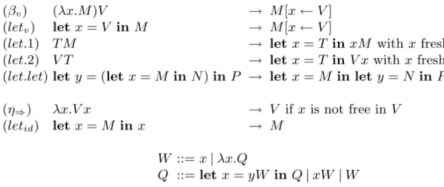
In [2], Moggi gives a call-by-value calculus, on the same syntax as λCBV. The

reduction rules and the grammar characterizing normal forms with respect to the (βv), (let.1), (let.2) and (let.let) rules are given in Figure 2 (T denotes terms

that are not values). This calculus was made to allow more reducing than the original call-by-value calculus while remaining call-by-value.

We say that two operational theories are in equational correspondence (see Sabry-Felleisen for the original notion [3]) if there is a bijection between the equivalence classes of the theories. Especially, we can show that our theory of λCBV is in equational correspondence with the one of Moggi.

5

(βv) (λx.M )V → M [x ← V ]

(letv) letx= V in M → M [x ← V ]

(let.1) T M → let x = T in xM with x fresh (let.2) V T → let x = T in V x with x fresh (let.let) let y = (let x = M in N ) in P → let x = M in let y = N in P (η⇒) λx.V x → V if x is not free in V

(letid) let x = M in x → M

W ::= x | λx.Q

Q ::= let x = yW in Q | xW | W

Fig. 2.Moggi’s λC-calculus and its normal forms

Proposition 7. The two calculi λc and λCBV are in equational correspondence.

Proof (Indication). We only show here the interesting cases of the simulation of the rules.

letapp= let.1 + let.let + (let.1)−1

letvar = let.2 + let.let + (let.2)−1

let.1 = (η_letletx=[] in N)−1

For let.2 we proceed case by case. If V is y, then let.2 = (ηletx[])

−1_{. If V = λy.M}

then let.2 =⇒ +(⇒)−1_.

Our claim is now that λCBV has a finer structure than λc. First, observe that

in Moggi’s calculus, for the same reason as in λCBV, the rules (βv) and (letv)

are sufficient for operational completeness.

Proposition 8. The λc-calculus restricted to the rules (βv) and (letv) is oper-ationally complete.

The λc-calculus equipped with (βv), (letv), (let.1), (let.2) and (let.let) is structurally complete.

A weird point is the presence of an observational rule, namely (η[]⇒) in the

simulation of the (let.1) and (let.2) rules, providing an ambiguous status to these two rules, used for computation but containing a bit of observation too. This can be related to another not so likable behavior of λc. We remember that the

calculus has the (βv) rule which is sufficient to reduce closed terms to values,

but if we reduce the term (λx.x)((λx.x)(λx.x)) with head reduction, we obtain the following reduction sequence:

(λx.x)((λx.x)(λx.x)) → let y = (λx.x)(λx.x) in (λx.x)y →∗

λx.x.

The head reduction uses the rule (let.2) as the first reduction rule, and for the term ((λx.x)(λxy.y))(λx.x)(λx.x) the head reduction uses the rules (let.1) and (let.let). So, even if we do not need them, these rules appear and the λc-calculus

tends to do useless expansions.

This was already noticed by Sabry and Wadler in [11] where they showed that λc is isomorphic to one of its sub-calculi where all the let rules have been

reduced, and applications occur only between two variables. The let construction is here a way to make the head-reduction flow explicit and to reduce a term, λc

firstly encodes its evaluation flow with some let manipulation, and only then reduces the term.

By doing this, we lose almost completely a “hidden agent” of the reduction : the structural congruence. In λv, the (βv) rule was sufficient because it could go

inside a term to find a redex, as here we almost never investigate in the term. The evaluation flow is encoded in a way that the topmost term always contains the redex, but is then superseding the structural congruence.

So, the status of the let rules is not clearly defined. They are used for reducing closed terms to values, but are also necessary for the structural completeness and contain a taste of observational rules.

Interestingly enough, we can switch between the normal forms or λC and

λCBV by using the η⇒E. Oriented from left-to-right we go from λC to λCBV and

conversely with the right-to-left orientation.

2

Call-by-value λµtp-calculus (λµtp

-calculus)

Our calculus is not hard to extend with continuation variables and control oper-ators. We follow the approach of [12] and adopt Parigot’s µ operator [9] together with a toplevel continuation constant tp, what simplifies the reasoning on closed computations and the connection with the λ-calculi based on callcc and A or Felleisen’s C operator. We write C[α ← [β]E] for the generalization of Parigot’s structural substitution and we abbreviate C[α ← [β]([ ])] as C[α ← β].

Since the reductions associated to µ absorb their context, structural rules should not change which subterm is in control, but happily structural rules are only like E[T ] → E′

[T ], so we cannot break confluence with them.

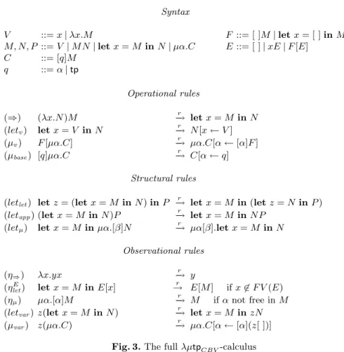
We must be careful with µ reductions however. If µ does not have any reduc-tion restricreduc-tions, let still can hide µ redexes. Therefore, we need a new structural rule. The full calculus is given in Figure 3.

Proposition 9. The operational subsystem, its extension with structural rules

and the full system of reduction rules are all confluent in the λµtpCBV-calculus.

Proof. The proof is the same as before, using generalizations of the rules involv-ing µ and let and with the parallel reduction extended with the two followinvolv-ing rules:

– if M ⇛ M′

then [α]M ⇛ [α]M′

– if C ⇛ C′

then µα.C ⇛ µα.C′

Note again the redundancy of (letvar) and (µvar) which are here for the

confluence.

As head reduction can be extended with the new rules, we obtain a notion of standardization for this calculus too.

Syntax V ::= x | λx.M F ::= [ ]M | let x = [ ] in M M, N, P ::= V | M N | let x = M in N | µα.C E::= [ ] | xE | F [E] C ::= [q]M q ::= α | tp Operational rules (⇒) (λx.N )M −→ let x = M in Nr (letv) letx= V in N r − → N [x ← V ] (µv) F[µα.C] r − → µα.C[α ← [α]F ] (µbase) [q]µα.C r − → C[α ← q] Structural rules (letlet) let z = (let x = M in N ) in P

r

−

→ let x = M in (let z = N in P ) (letapp) (let x = M in N )P

r − → let x = M in N P (letµ) letx= M in µα.[β]N r − → µα[β].let x = M in N Observational rules (η⇒) λx.yx r − → y (ηE

let) letx= M in E[x]

r → E[M ] if x 6∈ F V (E) (ηµ) µα.[α]M r − → M if α not free in M (letvar) z(let x = M in N )

r − → let x = M in zN (µvar) z(µα.C) r − → µα.C[α ← [α](z[ ])] Fig. 3.The full λµtpCBV-calculus

The rule letµ is here to deal with hidden µ-redexes, obfuscated by a let. As

an example, the term (let x = yz in µα.[α]λx.x)t needs first to be reduced to (µα.[α]let x = yz in λx.x)t, then only the reduction between µα and [ ]t can occur.

It is also interesting to see that being in call-by-value, we immediately dodge any problems with David and Py’s critical pair [13]. The term λx.(µα.c)x only reduces to λx.(µα.c[α ← [α][ ]x]), because of the η restriction to values.

We say that M evaluates to V in λµtp_CBV if [tp]M reduces to [tp]V and we say that a reduction relation → is operationally complete if whenever a closed M is not a value, [tp]M is reducible along → .

2.2 Normal forms

Not only do we keep the confluence, telling us that the extension is reasonable, but we also keep all the other good properties of the intuitionistic calculus. The grammar generating normal forms with respect to the operational and structural

rules, with T as an entry point, and the typing rules associated with the new µ construction are given in Figure 4 (T is a global parameter of the type system corresponding to the type of tp and all rules are generalized with a context ∆ on the right). Properties on the normal forms are preserved, as the proposition below says. S ::= x | ST Q::= λx.T | S | let x = S in Q T ::= Q | µα.[β]Q Γ ⊢ u : N | β : M, α : N, ∆ Γ ⊢ µβ.[α]u : M | α : N, ∆ Γ ⊢ u : T | β : M, ∆ Γ ⊢ µβ.[tp]u : M | ∆

Fig. 4.Normal forms and new typing rules for the λµtpCBV-calculus

Proposition 10. The λµtpCBV-calculus equipped with its set of operational rules is operationally complete and the λµtpCBV-calculus equipped with its sets of operational and structural rules is structurally complete.

If T is a term in normal form relatively to the operational and structural rules of λµtpCBV-calculus and Γ ⊢ T : A | ∆ then its proof satisfies the subformula property.

Proof (Indication). The first point is direct by the same proof as for the intuitionistic case. The second point is solved by induction, with most of the cases not being changed.

2.3 Equational theory

In [3], Sabry and Felleisen devised an equational theory of call-by-value λ-calculus with control operators that is sound and complete with respect to call-by-value continuation-passing-style (cps) semantics. We recall only the part of the equations concerning the control operators below, because the other one is verified by Moggi’s calculus and so by λCBV.

(Ccurrent) callcc (λk.kM ) = callcc (λkM )

(Celim) callcc(λd.M ) = M if d 6∈ F V (M )

(Clift) E[callcc M ] = callcc (λk.E[M (λf.(kE[f ]))])

if k, f 6∈ F V (E, M ) (Cabort) callcc(λk.C[E[kM ]]) = callcc (λk.C[kM ])

for C a term with a hole not binding k (Ctail) callcc(λk.((λz.M )N )) = λz.(callcc (λk.M ))N if k 6∈ F V (N )

(Abort) E[AM ] = AM

Because the language of the equations is not the same as ours, we need some translations: callcc and A are encoded by the terms (λx.µα.[α](x(λy.µδ.[α]y))) and λx.µδ.[tp]x while, conversely, we encode µα.[β]M by callcc (λkα.A(kβM)),

By unfolding the definitions and doing basic calculations, we obtain the equa-tional correspondence with the equations of Sabry and Felleisen. But instead of only having equations, we now have an oriented reduction system.

Proposition 11. There is an equational correspondence at the level of closed

expressions between λµtpCBV and Sabry and Felleisen’s axiomatization of λ-calculus with callcc and A.

Moreover, since we can equip λµtpCBV with a cps-semantics that matches

the one considered in Sabry and Felleisen as soon as µα.c is interpreted by λkα.c, [α]M by M kαand [tp]M by M λx.x, we can transfer Sabry and Felleisen

completeness result to the full theory of λµtpCBV.

Corollary 1. The full calculus λµtpCBV is sound and complete with respect to

βη along its cps-semantics.

Since tp has a passive role in the reduction system of λµtpCBV, the confluence

of the different subsystems and the structural and cps completenesses also hold for λµCBV which is λµtpCBV without tp.

Summary

We studied the equational theory of call-by-value λ-calculus and λµ-calculus from a reduction point of view and provided what seems to be the first confluent rewrite systems for λµ-calculus with control that is complete with respect to the continuation-passing-style semantics of call-by-value λ-calculus.

The rewrite system we designed is made of three independent blocks that respectively address operational completeness (ability to evaluate closed terms), structural completeness (ability to contract hidden redexes in open terms) and purely observational properties.

The notion of structural completeness is related to the ability to enforce the subformula property in simply-typed λ-calculus but we failed to find a purely computational notion that universally captures the subformula property. For instance, any call-by-value reduction system that does not use a let and does not smash abstraction and application from redexes of the form (λx.M )(yz) cannot be accompanied with a typing system whose normal forms type derivation satisfies the subformula property.

It would have been desirable to characterize the block of observational rules as a block of rules providing observational completeness, in a way similar to the call-by-name control-free case where β provides operational completeness and η provides observational completeness. Obtaining such a result would how-ever require a Böhm-style separability result for call-by-value λ-calculus and λµ-calculus, what goes beyond the scope of this study.

Regarding intuitionistic call-by-value λ-calculus we slightly refined Moggi and Sabry and Felleisen rewrite systems by precisely identifying which rules pertain to the operational block, the structural block or the observational block.

Finally, we proposed a new definition of standard reduction sequences for call-by-value λ-calculus that ensures the uniqueness of standard reduction paths between two terms (when such a path exists).

References

1. Plotkin, G.D.: Call-by-name, call-by-value and the lambda-calculus. Theor. Com-put. Sci. 1 (1975) 125–159

2. Moggi, E.: Computational lambda-calculus and monads. Technical Report ECS-LFCS-88-66, Edinburgh Univ. (1988)

3. Sabry, A., Felleisen, M.: Reasoning about programs in continuation-passing style. Lisp and Symbolic Computation 6(3-4) (1993) 289–360

4. Hofmann, M.: Sound and complete axiomatisations of call-by-value control oper-ators. Mathematical Structures in Computer Science 5(4) (1995) 461–482 5. Dezani-Ciancaglini, M., Giovannetti, E.: From Böhm’s theorem to observational

equivalences: an informal account. Electr. Notes Theor. Comput. Sci. 50(2) (2001) 6. Curien, P.L., Herbelin, H.: The duality of computation. In: Proceedings of ICFP

2000. SIGPLAN Notices 35(9), ACM (2000) 233–243

7. Herbelin, H.: C’est maintenant qu’on calcule: au cœur de la dualité. Habilitation thesis, University Paris 11 (December 2005)

8. Gentzen, G.: Untersuchungen über das logische Schließen. Mathematische Zeitschrift 39 (1935) 176–210,405–431 English Translation in The Collected Works of Gerhard Gentzen, Szabo, M. E. editor, pages 68-131.

9. Parigot, M.: Lambda-mu-calculus: An algorithmic interpretation of classical natu-ral deduction. In: International Conference LPAR ’92 Proceedings, St. Petersburg, Russia, Springer-Verlag (1992) 190–201

10. Regnier, L.: Une équivalence sur les lambda-termes. Theor. Comput. Sci. 126(2) (1994) 281–292

11. Sabry, A., Wadler, P.: A reflection on call-by-value. ACM Trans. Program. Lang. Syst. 19(6) (1997) 916–941

12. Ariola, Z.M., Herbelin, H.: Control reduction theories: the benefit of structural substitution. Journal of Functional Programming 18(3) (May 2008) 373–419 with a historical note by Matthias Felleisen.

13. David, R., Py, W.: Lambda-mu-calculus and Böhm’s theorem. J. Symb. Log. 66(1) (2001) 407–413