HAL Id: hal-03254145
https://hal.archives-ouvertes.fr/hal-03254145
Submitted on 9 Jun 2021
HAL is a multi-disciplinary open access
archive for the deposit and dissemination of
sci-entific research documents, whether they are
pub-lished or not. The documents may come from
teaching and research institutions in France or
abroad, or from public or private research centers.
L’archive ouverte pluridisciplinaire HAL, est
destinée au dépôt et à la diffusion de documents
scientifiques de niveau recherche, publiés ou non,
émanant des établissements d’enseignement et de
recherche français ou étrangers, des laboratoires
publics ou privés.
Distributed under a Creative Commons Attribution| 4.0 International License
Active red giants: Close binaries versus single rapid
rotators
Patrick Gaulme, Jason Jackiewicz, Federico Spada, Drew Chojnowski, Benoît
Mosser, Jean Mckeever, Anne Hedlund, Mathieu Vrard, Mansour Benbakoura,
Cilia Damiani
To cite this version:
Patrick Gaulme, Jason Jackiewicz, Federico Spada, Drew Chojnowski, Benoît Mosser, et al.. Active
red giants: Close binaries versus single rapid rotators. Astronomy and Astrophysics - A&A, EDP
Sciences, 2020, 639, pp.A63. �10.1051/0004-6361/202037781�. �hal-03254145�
https://doi.org/10.1051/0004-6361/202037781 c P. Gaulme et al. 2020
Astronomy
&
Astrophysics
Active red giants: Close binaries versus single rapid rotators
?
Patrick Gaulme
1,2, Jason Jackiewicz
2, Federico Spada
1, Drew Chojnowski
2, Benoît Mosser
3, Jean McKeever
4,
Anne Hedlund
2, Mathieu Vrard
5,6, Mansour Benbakoura
7,8, and Cilia Damiani
11 Max-Planck-Institut für Sonnensystemforschung, Justus-von-Liebig-Weg 3, 37077 Göttingen, Germany
e-mail: [email protected]
2 Department of Astronomy, New Mexico State University, PO Box 30001, MSC 4500, Las Cruces, NM 88003-8001, USA
3 LESIA, Observatoire de Paris, Université PSL, CNRS, Sorbonne Université, Université de Paris, 92195 Meudon, France
4 Department of Astronomy, Yale University, PO Box 208101, New Haven, CT 06520-8101, USA
5 Department of Astronomy, The Ohio State University, 140 West 18th Avenue, Columbus, OH 43210, USA
6 Instituto de Astrofísica e Ciências do Espaço, Universidade do Porto, CAUP, Rua das Estrelas, 4150-762 Porto, Portugal
7 IRFU, CEA, Université Paris-Saclay, 91191 Gif-sur-Yvette Cedex, France
8 Université Paris Diderot, AIM, Sorbonne Paris Cité, CEA, CNRS, 91191 Gif-sur-Yvette Cedex, France
Received 20 February 2020/ Accepted 24 April 2020
ABSTRACT
Oscillating red-giant stars have provided a wealth of asteroseismic information regarding their interiors and evolutionary states, which enables detailed studies of the Milky Way. The objective of this work is to determine what fraction of red-giant stars shows photometric rotational modulation, and understand its origin. One of the underlying questions is the role of close binarity in this population, which relies on the fact that red giants in short-period binary systems (less than 150 days or so) have been observed to display strong rotational modulation. We selected a sample of about 4500 relatively bright red giants observed by Kepler, and show that about 370 of them (∼8%) display rotational modulation. Almost all have oscillation amplitudes below the median of the sample, while 30 of them are not oscillating at all. Of the 85 of these red giants with rotational modulation chosen for follow-up radial-velocity observation and analysis, 34 show clear evidence of spectroscopic binarity. Surprisingly, 26 of the 30 nonoscillators are in this group of binaries. On the contrary, about 85% of the active red giants with detectable oscillations are not part of close binaries. With the help of the stellar masses and evolutionary states computed from the oscillation properties, we shed light on the origin of their activity. It appears that low-mass red-giant branch stars tend to be magnetically inactive, while intermediate-mass ones tend to be highly active. The opposite trends are true for helium-core burning (red clump) stars, whereby the lower-mass clump stars are comparatively more active and the higher-mass ones are less active. In other words, we find that low-mass red-giant branch stars gain angular momentum as they evolve to clump stars, while higher-mass ones lose angular momentum. The trend observed with low-mass stars leads to possible scenarios of planet engulfment or other merging events during the shell-burning phase. Regarding intermediate-mass stars, the rotation periods that we measured are long with respect to theoretical expectations reported in the literature, which reinforces the existence of an unidentified sink of angular momentum after the main sequence. This article establishes strong links between rotational modulation, tidal interactions, (surface) magnetic fields, and oscillation suppression. There is a wealth of physics to be studied in these targets that is not available in the Sun.
Key words. binaries: spectroscopic – stars: rotation – stars: oscillations – techniques: radial velocities – techniques: photometric – starspots
1. Introduction
Thanks to the observations of the space photometers CoRoT (Baglin et al. 2009), Kepler (Borucki et al. 2011), and now TESS (Ricker et al. 2015), red giant (RG) stars are known to commonly display solar-like (SL) oscillations (De Ridder et al. 2009). As for main-sequence (MS) SL stars, these global oscillations are stochastically excited by turbulent convection in their outer con-vective envelopes. From a revised classification of the Kepler tar-gets (Berger et al. 2018) based on the second data release of the ESA Gaia mission (Gaia Collaboration et al. 2018) and using the revised temperatures from the Kepler Stellar Properties Catalog (KSPC DR25, Mathur et al. 2017),Hon et al.(2019) detected oscillations in about 92% of the 21 000 RGs observed by the
? Full Table C.1 is only available at the CDS via anonymous ftp
tocdsarc.u-strasbg.fr(130.79.128.5) or viahttp://cdsarc. u-strasbg.fr/viz-bin/cat/J/A+A/639/A63
original Kepler mission. We note that this fraction is much higher than the 40% detection rate reported for MS SL stars (Chaplin et al. 2011;Mathur et al. 2019), whose light curves are domi-nated by observational noise (Mosser et al. 2019). Asteroseis-mology is thus a very powerful tool to analyze the evolution of stars after the MS as it can be performed on almost all targets of vast samples of stars.
Contrarily to MS SL stars (e.g.,García et al. 2014a), only a few percent of the RGs show a pseudo-periodic photometric variability likely originating from surface spots (Ceillier et al. 2017), which we hereafter call “rotational modulation”. The most commonly adopted explanation is that RGs are slow rotators (e.g.,Gray 1981;de Medeiros et al. 1996) where no significant dynamo-driven magnetic fields are generated in their large con-vective envelope, implying no detectable surface spots. In this respect, it is worth noticing that no direct detection of magnetic field has been reported so far for stars on the red giant branch (RGB) with masses below 1.5 M (Charbonnel et al. 2017).
Open Access article,published by EDP Sciences, under the terms of the Creative Commons Attribution License (https://creativecommons.org/licenses/by/4.0), which permits unrestricted use, distribution, and reproduction in any medium, provided the original work is properly cited.
Nevertheless, measuring the rotation rate of RG stars is of prime importance to understand the evolution of stellar rotation after the MS. For this reason, much effort has lately been devoted to measure their rotation rates from their radiative cores (e.g.,Beck et al. 2012;Mosser et al. 2012a;Deheuvels et al. 2015;Gehan et al. 2018) to their surfaces (e.g.,Carlberg et al. 2011; Costa et al. 2015; Deheuvels et al. 2015; Tayar et al. 2015; Ceillier et al. 2017).
From high-resolution (HR) spectroscopic measurements of projected rotational velocities v sin i by Carlberg et al.(2011), about 2% of RGs are rapid rotators, using a threshold of v sin i= 10 km s−1as is commonly adopted in the literature (e.g.,Drake et al. 2002; Massarotti et al. 2008; Costa et al. 2015; Tayar et al. 2015). Although the details of stellar dynamo theory are not yet fully understood, the empirical correlation between mag-netic activity and rotation (e.g., Noyes et al. 1984) lends sup-port to the expectation that the fraction of stars with detected rotational modulation should be similar to those with rapid rota-tion (see alsoCeillier et al. 2017). Despite this correlation, as of yet there is no theoretical calculation that finds the condition for spot generation to be v sin i ≥ 10 km s−1. However,Ceillier et al.
(2017) reported the detection of starspot variability in about 2% of the light curves from a systematic search in the Kepler oscil-lating RGs, which matches the fraction of rapid RG rotators of
Carlberg et al.(2011). In the rest of the paper, we consider that RGs with rotational modulation are fast rotators relatively to the bulk of RG stars.
Currently, the observed rotation in both intermediate and low mass stars present puzzling features compared with the standard theoretical predictions. Intermediate mass stars (M ∈ [1.5−3] M ) do not have a convective envelope during the MS,
which means no large scale magnetic fields, and hence no angu-lar momentum loss during it (e.g., Durney & Latour 1978;
Tayar et al. 2015). The rotation periods of A and late B-type stars cover a very broad range during the MS up to v sin i ∼ 300 km s−1(Zorec & Royer 2012). When the rapid rotators reach the RGB, they develop a convective envelope while still spin-ning fast, and they keep having a significantly large rotation (v sin i ≥ 10 km s−1) during the subsequent core-helium-burning
stage, also known as the red clump (RC) in reference to the color-magnitude diagram (e.g.,Girardi 2016). This theoretical expec-tation is actually not observed in practice:Ceillier et al.(2017) find 1.9% of M ≥ 2 M RGs with rotational modulation, and Tayar & Pinsonneault(2018) report a distribution of v sin i peak-ing between 3 and 5 m s−1 with maximum values at 10 km s−1. As regards low-mass stars (M ≤ 1.3 M ), which have convective
envelopes and thus lose angular momentum during the MS, we expect slow rotation rates when they evolve. From stellar evo-lution models, Tayar et al.(2015) indicate that low-mass stars should show v sin i ≤ 0.3 km s−1during the RGB, and at
max-imum an order of magnitude larger on the RC. Surprisingly, measurements of v sin i byTayar et al.(2015) and photometric modulation by Ceillier et al.(2017) reported that between 7% and 15% of RGs with masses M ≤ 1.1 M are fast rotators. Such
low-mass rapidly rotating RGs are thus suspected to have either been spun up by tidal interactions with a stellar companion, or have merged with or engulfed a stellar or substellar companion.
In parallel to this, it has also been observed that RGs in close eclipsing binary (EB) systems have peculiar photometric properties (Gaulme et al. 2014). Among the 35 Kepler RGs that are confirmed to belong to EBs, 18 display regular solar-like oscillations – with their amplitudes matching the empirical expectations (e.g.,Kallinger et al. 2014) – and no rotational ulation. All of the remaining systems display rotational
mod-ulation, seven with partially suppressed oscillations, and ten do not have detectable oscillations (Gaulme et al. 2014,2016;
Benbakoura et al. 2020).Gaulme et al.(2016) showed that the nondetection of oscillations is not an observational bias. This is observed in the closest systems, where most orbits are circular-ized, and rotation periods are either synchronized or in a spin-orbit resonance. Such a configuration is observed for systems whose orbital periods are shorter than about Porb∼ 150 days, and
the sum of the stellar radii relatively to the system’s semi-major axis (R1+ R2)/a& 7% of the semi-major axis. In the following,
we consider a binary system to be close when Porb. 200 days. Gaulme et al.(2014) suggested that the surface activity and its concomitant mode suppression originate from tidal interactions. During the RGB, close binary systems reach a tidal equilib-rium where stars are synchronized and orbits circularized (e.g.,
Verbunt & Phinney 1995; Beck et al. 2018). Red giant stars are spun up during synchronization, which leads to the devel-opment of a dynamo mechanism inside the convective enve-lope, leading to surface spots. The magnetic field in the envelope likely reduces the turbulent excitation of pressure waves by par-tially inhibiting convection. Since spots can also absorb acoustic energy, these two effects lead to the suppression of oscillations.
This phenomenon observed with RGs in EBs led us to hypothesize that a large fraction of the RGs with rotational modulation – hereafter “active” RGs – and suppressed oscilla-tions actually belong to short-period (noneclipsing) binary sys-tems. This connection between fast rotating RGs and binarity has been considered for a long time (e.g., Simon & Drake 1989;
Carlberg et al. 2011), but no dedicated observations have been led to test it. Only archived data from large surveys were con-sidered in recent works (Tayar et al. 2015;Ceillier et al. 2017), leading to rather inconclusive results on that matter.
The goal of the present paper is firstly to determine what fraction of active RGs are in close binary systems, and secondly to understand the origin of magnetic activity in the RGs that do not belong to close binaries. We base our work on a self-consistent approach where we select a sample of about 4500 RGs observed by Kepler that are not known to belong to any binary system, and that are expected to exhibit SL oscillations (Sect.2). Among them, we show that about 370 (≈8%) display signifi-cant rotational modulation, which appears to be correlated with weak oscillations (Sect. 3.1). We then look for radial velocity (RV) variability in a subset of 85 targets from HR spectroscopic measurements (Sect.3.2), and find a significant fraction of spec-troscopic binaries (SBs). In the last Sect.3.3, we classify and quantify the possible scenarios that could have led to the active RGs that are not in binary systems.
2. Data and methods
2.1. A sample of 4500 RGs observed by Kepler
The first step of our work consists of measuring the fraction of RGs displaying clear rotational modulation, and reassess-ing the correlation between rotational modulation and suppres-sion of SL oscillations pointed out by García et al. (2010),
Chaplin et al. (2011), Gaulme et al. (2014), or Mathur et al.
(2019), for instance. Our main concern at this step is to avoid observational biases by including targets that are not suit-able for our study. We started from the updated RG catalog of Berger et al. (2018), and selected a subsample of targets whose oscillations should be detectable provided that they are regular RGs. We base our selection criterion on the conclu-sions ofMosser et al.(2019), who quantified the asteroseismic
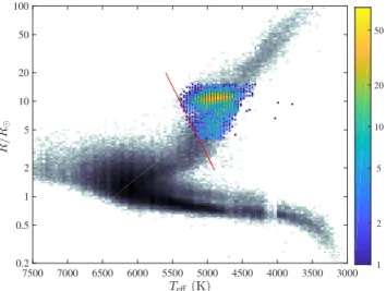
3000 3500 4000 4500 5000 5500 6000 6500 7000 7500 0.2 0.5 1 2 5 10 20 50 100 1 2 5 10 20 50
Fig. 1.Radius-temperature diagram of the stars available inBerger et al.
(2018) in the range [0.2, 100] R and [3000, 7500] K. Radii are from
Gaiaand temperatures from the Kepler MAST archive. Temperature
axis is reverse, that is with higher Teff toward left. Color-coding
repre-sents logarithmic number density. The colored part of the diagram indi-cates the location of our sample. The red line indiindi-cates the limit between
subgiant and giant stars according toBerger et al.(2018), such as the
RGs lay at the top-right corner. According toBerger et al.(2018), the
discontinuity in Teff near 4000 K is an artifact due to systematic shifts
in Teffscales in the DR25 Kepler Stellar Properties Catalog.
performance of Kepler as a function of apparent magnitude and observation duration. This led us to consider RGs with Kepler magnitude mKep ≤ 12.5 and observation duration longer than
13 quarters (≈3 years). We also limit ourselves to RGs with radii less than 15 R to avoid being biased by targets whose
oscilla-tions at maximum amplitude are at frequencies νmax . 15 µHz,
which could be filtered out during light-curve processing. We also exclude those with radii less than 4 R to avoid
oscilla-tion modes beyond Kepler’s long-cadence Nyquist frequency (≈283 µHz). We note that 75% of the Kepler RG sample have radii between 4 and 15 R . In other words we focus on the
“main-stream” RGs. A total of 4580 out of the ≈21 000 RGs meet these criteria (See Fig.1).
As misclassification can happen in large catalogs, we excluded stars that were clearly not single RGs from a visual inspection of the Kepler light curves and their frequency spectra. This downselection filtered out obvious binary systems as dou-ble RG oscillators, eclipsing binaries, ellipsoidal binaries, and highly eccentric noneclipsing binaries (“heartbeat stars”, e.g.,
Welsh et al. 2011;Beck et al. 2014), but also classical pulsators as δ Scuti or γ Doradus. We found 88 light curves including a binary signal, and 21 with either a δ Scuti or a γ Doradus pul-sator. We identified another 6 with a damaged Kepler light curve, that is where photometry is clearly wrong. We thus ended up with a sample of 4465 stars classified as RGs according toBerger et al.(2018) and with no obvious indication of misclassification or peculiarity.
2.2. The Kepler light curves
We primarily worked with the Kepler public light curves that are available on the Mikulski Archive for Space Telescopes (MAST)1. Two types of time series are available: the Simple
Aperture Photometry (SAP) and the Pre-search Data
Condition-1 http://archive.stsci.edu/kepler/
ing Simple Aperture Photometry (PDC-SAP) light curves. The latter consist of time series that were corrected for discontinu-ities, systematic errors and excess flux due to aperture crowding (Twicken et al. 2010). They do not meet our requirements for monitoring the rotational modulation, which is often removed during the process (e.g.,García et al. 2014b;Gaulme et al. 2014). We thus made use of the SAP data to preserve any possible long-term signal. This choice entails our own detrending and stitching operation on the light curves while ensuring that the rotational modulation is preserved after each interruption of the time series. The methods employed to clean the time series are detailed in
Gaulme et al.(2016).
To reinforce our results – especially the flagging of rota-tional modulation and the measurement of rotarota-tional periods – we repeated the whole light processing and analysis with the public Kepler Light Curves Optimized For Asteroseismology (KEPSEISMIC,García et al. 2011;Pires et al. 2015)2, which are optimized for asteroseismic analysis. KEPSEISMIC light curves were available for 4444 out of the 4465 targets. Except for a few cases, the results obtained with either light curves were in agree-ment. In the following, our results reflect the final analysis done by working both the SAP and KESPSEISMIC time series. 2.3. Surface rotation periods
In a first step, the presence of rotational modulation is automati-cally searched, before being checked by visual inspection. Rota-tional modulation is considered whenever the standard deviation of the photometric time series is larger than 0.1%. We note that this definition is equivalent to the photometric index Sphdefined
by Mathur et al. (2014) in the case no photometric period is measured. Then from both the power spectrum and the autocor-relation of the times series, the algorithm automatically checks for surface activity, and provides an estimate of its fundamen-tal period in case of positive detection. Rotational modulation is considered for periods ranging from 1 to 180 days. From the power spectrum, peaks are considered to be significant when the statistical null hypothesis test is less than 1% with respect to the average background noise level. Autocorrelation is used to check the estimate obtained from the power spectrum, by verifying that the highest peak lies in the same period range within a factor 1/2 or 2, as misestimates can happen. Visual inspection was then used to decide the actual rotation period in case of disagreement between power spectrum and autocorrelation periods.
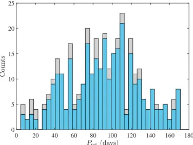
Beyond measuring rotation periods, we need to be care-ful with possible photometric contamination from nearby stars. Indeed, it can happen that a considered RG does not have any spot but that a neighboring MS stars display spots and that the light curves leak into each other.Ceillier et al.(2017) tracked this possible source of errors by making use of the crowding param-eter available on the Kepler database at MAST. The crowding parameter is defined as the fraction of the flux coming from the considered target in the light curve. The lower the crowd-ing parameters, the higher the chance of contamination. In their case, they considered all the 17 377 RGs with detected oscilla-tions at the time, which included many faint targets. Their Fig. 5 shows the comparison between the histogram of rotational peri-ods with and without targets where the crowding factor is less than 0.98. In their case, they found that the targets with low crowding represent 32% of their active RG sample, and are a significant source of bias as they constitute a clear group of outlying Prot with values less than 30 days. In our case, Fig.2
0 20 40 60 80 100 120 140 160 180 0 5 10 15 20 25
Fig. 2. Histogram of the rotation periods Prot that we measure for
340 RGs where both oscillations and rotation are detected. The gray histogram includes all targets, whatever their crowding factor. The blue histogram includes only the 305 targets with crowding larger than 0.98.
This figure echoes Fig. 5 ofCeillier et al.(2017).
shows that the stars with a crowding factor less than 0.98 (13% of our active RGs) do not constitute a well defined group, so we can legitimately consider that targets with a lower crowding fac-tor are not due to contamination in most cases, and that we are not affected by this problem. It is not surprising since we focus on purpose on the brightest part of the sample to avoid observa-tional biases of that kind.
2.4. Oscillation analysis
The detection of oscillations is based on the envelope of the autocorrelation function (EACF) developed byMosser & Appourchaux(2009), which we apply to the power spectrum of the time series (Fig.3panel i). A first run of the EACF leads to initial estimates of the mean frequency separation∆ν and νmax,
independently from the background noise level. The second step consists of refining∆ν and νmaxby taking into account the
back-ground noise.
The stellar granulation and accurate values of νmaxand mode
amplitude Hmax are estimated by fitting the power spectrum
as commonly performed in asteroseismology (Kallinger et al. 2014), and already used in Gaulme et al. (2016). Following
Kallinger et al. (2014), the power density spectrum is fitted by the following function:
S(ν)= N(ν) + η(ν) [B(ν) + G(ν)] , (1)
where the N is the function describing the noise, η is a damping factor originating from the data sampling, B is the sum of three “Harvey” functions (super Lorentzian functions centered on 0), and G is the Gaussian function that accounts for the oscillation excess power: G(ν)= Hmaxexp " −(ν − νmax) 2 2σ2 # . (2)
The terms νmaxand Hmaxare the central frequency and height of
the Gaussian function.
A second estimate of ∆ν is performed again with EACF from the whitened power spectral (power spectrum divided by
background function). Oscillations are considered to be detected when both the maximum value of the EACF is larger than 8 (Mosser & Appourchaux 2009) and peaks are visible in the spec-trum. We then compute the stellar masses and radii thanks to the asteroseismic scaling relations that were originally proposed byKjeldsen & Bedding(1995) for SL MS oscillators, and then successfully applied to RGs (e.g.,Mosser et al. 2013). The stel-lar effective temperatures, also needed in the scaling relations, are those from the Kepler Gaia data release 2 with their corre-sponding errors. We employ the asteroseismic scaling relations as proposed by Mosser et al. (2013) for RGs, that is, where νmax, = 3104 µHz, ∆ν = 138.8 µHz, Teff, = 5777 K, and
where the observed∆ν is converted into an asymptotic one, such as∆νas= 1.038 ∆ν.
In addition to the properties of the pressure p modes (νmax,
∆ν) we analyze the properties of the mixed modes, which result of the interaction between the p-modes that resonate in the con-vective envelope and the gravity g modes that resonate in the radiative core. At first order, p modes are evenly spaced by∆ν as a function of frequency, whereas g modes are evenly spaced by∆Π as a function of period. From the dipole (l = 1) mixed modes it is possible to measure the mean period spacing of the dipole g modes∆Π1, which is related to the physical properties
of the core. For RGs this information is precious as it allows us to unambiguously distinguish the H-shell (RGB) from the He-core (RC) burning stars. Since the CoRoT space mission, such a type of analysis is commonly performed with RG stars (Bedding et al. 2011; Mosser et al. 2011; Stello et al. 2013). According to (Mosser et al. 2014) when ∆ν ≥ 9.5 µHz, we assume the stars to be on the RGB. When mixed modes are detectable, the evolutionary status is determined according to the methods described inVrard et al.(2016). Overall, we have the status of 3405 stars out of the 4465: we used 2307 published statuses that were already available inVrard et al.(2016), and we determined the status of 1098 others. Figure 4 shows the period spacing of the dipole mixed modes ∆Π1 as a function
of the large frequency separation∆ν for the subsample of active RGs. We note a larger dispersion of the period spacing∆Π1for
RGBs with∆ν ≤ 7 µHz. This issue is well known (Dupret et al. 2009;Grosjean et al. 2014): RGBs with low∆ν are more evolved than those with larger values, and the coupling between p and g modes is less efficient. Hence, gravity-dominated mixed modes display lower signal-to-noise ratio.
Finally, our analysis of the oscillation spectra also considers the question of the RGs with depleted dipole modes (e.g.,Mosser et al. 2012b;García et al. 2014b), which is possibly caused by the presence of fossil magnetic fields in radiative cores of interme-diate mass RGs that had convective cores during the MS (Fuller et al. 2015;Stello et al. 2016;Mosser et al. 2017). Despite the suppression of dipole modes is a priori not related to rotational modulation – the former is supposed to be caused by core mag-netic fields, the latter by surface ones –, we thought it was inter-esting to flag it in case of an unlikely correlation. We applied the method presented byMosser et al.(2012b) to measure the rela-tive visibilities of the modes of degrees l= 0, 1, 2, and 3 to the whole sample, whenever oscillations were detected (see Fig.5). 2.5. A dedicated pipeline to analyze the sample
We developed an automatic pipeline – the Data Inspection Tool, hereafter DIT – to analyze the whole sample, which cleans the light curves and extracts the properties of both rotational mod-ulation and solar-like oscillations. The code is similar to that described inGaulme & Guzik(2019) to look for stellar pulsators
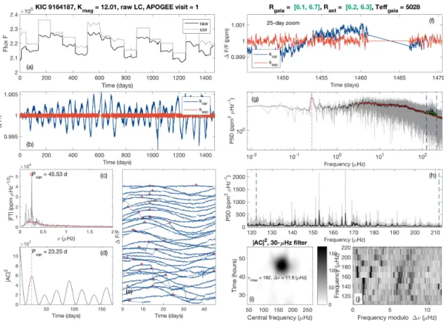
Fig. 3.Data inspection tool applied to the RGB star KIC 9164187, which shows surface activity and oscillations, including mixed dipole modes. Left column from top to bottom. Panel a: Kepler light curves as a function of time, where “raw” stands for SAP and “cor” for PDCSAP. Panel b:
light curves expressed in relative fluxes∆F/F, where the blue line contains the stellar activity and oscillations, and the red curve is optimized
for oscillation search (activity filtered out). Panel c: fourier spectrum of the time series, where the highest peak and its corresponding period is
indicated in days. Panel d: square of the autocorrelation |AC|2of the time series, where the highest correlation is indicated and expressed in days.
Panel e: light curve folded on the dominant variability period, where a vertical shift between consecutive multiples of the rotational period was introduced. Right column from top to bottom. Panel f: zoom of the light curve over 25 days. Panel g: log-log scale display of the power spectral
density of the time series (gray line) expressed in ppm2µHz−1as a function of frequency (µHz). The black line is a smooth of it (boxcar) over
100 points. The solar-like oscillations appear as an excess power between the two dashed blue lines. The plain red line represents the model of the stellar background noise and the green line is the Gaussian function used to model the oscillation power. The vertical dashed line indicates the peak corresponding to the rotational modulation determined in panel c. Panel h: power density spectrum of the time series as a function of
frequency centered around νmax(here ≈162 µHz). Panel i: envelope of the autocorrelation function (EACF) as a function of frequency and time.
The dark area corresponds to the correlated signal – i.e., the oscillations – where its abscissa indicates νmaxand its ordinate 2/∆ν. Panel j: échelle
diagram associated with the large frequency spacing automatically determined from the EACF plot. The power density spectrum is smoothed by a
boxcar over three bins and cut into∆ν = 11.9 µHz chunks; each is then stacked on top of its lower-frequency neighbor. This representation allows
for visual identification of the modes. Darker regions correspond to larger peaks in power density. The x-axis is the frequency modulo the large
frequency spacing (i.e., from 0 to∆ν), and the y-axis is the frequency.
in eclipsing binaries. Beyond the measurements of rotational modulation, background and oscillations, the DIT produces a vetting sheet for each target that includes a series of figures allowing the user to appreciate the quality of the measurements. An example of vetting sheet is displayed in Fig.3.
All vetting sheets were visually inspected. The objective of the visual inspection was to double check the detection of rota-tional modulation, assess the value of the rotation period, and look for oscillations that had been missed by the DIT. Besides, it allowed us to exclude the obvious binaries and classical pul-sators as explained in the previous section. Regarding rotational modulation, we did not strictly stick to the Sph≥ 0.1% threshold,
as some photometric discontinuities could cause Sphlarger than
that. Besides, some actual photometric modulation could have lower Sph. The distinction between a spurious photometric
mod-ulation, arising from imperfect light curve cleaning, and actual stellar signal was most of the time clear. However, in conditions of low signal-to-noise ratio (S/N), flagging the detection of
stel-lar activity could be fragile. This is why we used two classes of flags for activity: clear and ambiguous detection (see Sect.3.1). 2.6. High-resolution spectroscopy
As indicated in the introduction, we study a subsample of RGs displaying rotational modulation with HR spectroscopy to look for RV variability. Our intend is not to perform a detailed anal-ysis of these spectra such as retrieving chemical composition or vsin i, which will be part of a future work.
From October 2018 to June 2019, we were granted time on the échelle spectrometer of the 3.5 m telescope of the Astro-physical Research Consortium (ARC) at Apache Point obser-vatory (APO), which covers the whole visible domain at an average resolution of 31 000. This time allowed us to monitor a set of 51 RGs with clear rotational modulation. Even though the ARC échelle spectrometer was not designed for fine RV measurements, it has successfully been used for this purpose in
2 4 6 8 10 12 14 16 18 20 22 0 50 100 150 200 250 300 350 400 RGB RC 1 1.5 2 2.5 3
Fig. 4.Period spacing of the l = 1 mixed modes ∆Π1 (expressed in
seconds) as a function of the large frequency separation∆ν (expressed
in µHz). The period spacing is measured for 3388 stars out of the sample of 4465 RGs. The colors of the markers indicate the stellar masses as
indicated in the colorbar (deep blue is less that 1.5 M ). The dashed line
separates the red clump stars (above) and the RGBs (below).
0 5 10 15 20 25 0 0.2 0.4 0.6 0.8 1 1.2 1.4 1.6 1.8
Fig. 5.Visibility of dipole modes of the sample. Under the black line,
l= 1 modes are considered to be depleted.
earlier works about RGs (e.g.,Rawls et al. 2016;Gaulme et al. 2016). The measurement error reported in these papers is about 0.5 km s−1 for an RG spectrum with S /N between 10 and 20.
In practice our spectra have S/N ranging from 10 to 25. With ARCES data, we thus consider a target to be an SB when the dis-persion is larger than σRV= 2 km s−1. The ARCES Optical
spec-tra were processed and analyzed in the same way as inGaulme et al.(2016) and we refer to this paper for details.
Beyond the ARC telescope, we used infrared high-resolution spectroscopic data of another 34 targets that were available in the archived data (release 16, Ahumada et al. 2019) of the APO Galactic Evolution Experiment (APOGEE,Majewski et al. 2017), which is part of the Sloan Digital Sky Survey IV (e.g.,
Blanton et al. 2017). Regarding APOGEE data, we directly use the archived RVs. This spectrometer has an average resolution of 22 500 and is known to be stable, with a noise level lower than 0.1 km s−1(Deshpande et al. 2013). Knowing that the RV
0 5 10 15 20 25 0 50 100 150 200
Fig. 6. Rotation period Prot as a function of the mean large spacing
∆ν for RGs displaying both rotational modulation and oscillations. The
gray line indicates the critical period Tcritand the red line a rotational
velocity of 80% of Tcrit. Blue squares are the RGs with clear rotational
modulation, blue circles those with low S /N detection. Orange symbols indicate the same for those with crowding factor less than 0.98. This
figure echoes Fig. 4 ofCeillier et al.(2017).
jitter of RGs with surface gravities 2 ≤ log g ≤ 3 – as we have here – is less than 0.1 km s−1(Hekker et al. 2008), we
con-sider an RG to be an SB when the RV dispersion is larger than σRV= 0.5 km s−1.
3. Results
3.1. Occurrence of red giants with rotational modulation Among the 4465 RG stars that we have selected, our main con-clusions regarding their Kepler light curves are the following.
Firstly, a total of 298 RGs display clear rotational modu-lation, that is, in 6.65% of the cases. For another 73 targets (1.63%), the detection of surface activity is ambiguous (low S/N). If we assume the ambiguous detections as a proxy of our error in judgment, we can consider that 7.5 ± 0.8% of the RGs display rotational modulation. We thus detect from three to four times more RGs with rotational modulation than the 2% reported byCeillier et al.(2017). As indicated in Sect.2.3, the main dif-ference with their work is that they considered the whole sam-ple of oscillating RGs known at the time, which included faint stars and likely discarded stars with suppressed oscillations. By comparing Fig.6with Fig. 4 ofCeillier et al.(2017), we clearly detect more stars in the∆ν range [6.5, 9.5] µHz, which contains many intermediate-mass RCs.
Secondly, we detect oscillations in 99.32% of our sample, that is in all except 30, which is much more than previously reported. This difference is not surprising because Hon et al.
(2019) considered the whole 21 000 RG catalog which contains faint stars, including crowded fields. Besides, their automatic pipeline may have encountered difficulties when dealing with low S /N oscillation spectra, especially in the presence of rota-tional modulation. We interestingly note that the fraction 8% of RGs whereHon et al.(2019) do not detect oscillations is equal to the fraction of our RGs displaying activity.
Thirdly, all of the 30 targets with no detectable oscillations display a significant rotational modulation. In other words, if an RG does not oscillate, rotational modulation is always detected.
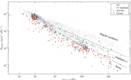
20 30 50 100 200 101 102 103 104 Regular oscillators Depleted l=1 Active All l=1 depleted Activity Unsure
Fig. 7. Oscillation height Hmax
(ppm2µHz−1) as a function of the
frequency at maximum amplitude νmax
(µHz) of the 4465 red giants considered in this work, minus the 30 for which no oscillations were detected, that is
4435 total. The parameter Hmax is the
height of the Gaussian function used to fit the oscillation contribution to the power spectral density. The frequency
at maximum amplitude νmax is the
center of the same Gaussian function. Light gray points indicate all the targets,
green are l = 1 depleted, red squares
are the systems with significant surface activity, and blue circles indicate the cases of ambiguous detection of surface activity.
Fourthly, almost all the active RGs display unusually low-amplitude oscillations, as well as most of those with ambiguous status. This can be seen in Fig.7, which plots a proxy of the oscillation amplitude – the height Hmaxof the Gaussian function
employed to fit the oscillation envelope in the power spectral density of the time series – as a function of νmax. We distinguish
three groups of oscillators: the regular, the dipole-depleted, and the active ones. The dipole-depleted RGs appears as a distinct group because if l = 1 modes are absent, the oscillation power that we fit with a Gaussian function is reduced3.
Finally, measurements of dipolar mode visibilities as per-formed inMosser et al.(2012b,2017) reveal that 17% and 10% of inactive and active RGs display l= 1 depleted modes, respec-tively. To complement these results, a visual flagging of depleted dipole modes led us to identify 12% and 20% in the same two groups. We conclude that the fraction of depleted dipolar-mode oscillators is very similar in both samples of inactive and active RGs (Fig.7), and cannot be considered as a significant source of biases in our analysis.
3.2. Occurrence of close binaries among the active red giants
According to the previous section, 7.5 ± 0.8% of the RGs display rotational modulation. We now determine how many of them actually belong to close binary systems thanks to multi-epoch high-resolution spectroscopic measurements.
The rate of SBs actually represents a lower limit of the frac-tion of close binaries because some systems are seen almost pole-on and display very low line-of-sight velocities. However, the RV semi-amplitude of the typical binary system that we expect – synchronized, circularized, period of about 50 days, solar masses – is larger than about 5 km s−1in 90% of the cases, by assuming random inclination angles (see Appendix A). In addition, we show that five measurements randomly distributed over a 200-day range with at least seven days between consec-utive observations are very likely to detect RV variability. With the ARCES spectrometer, we observed four times most of our targets, and up to seven times some targets whose RV variability
3 Dipole-depleted RGs would not appear as a distinct group if our
proxy of the oscillation amplitude were the amplitude of radial modes.
Oscillating Nonoscillating 0 10 20 30 40 RV stable SB Unsure Test Sample 0 50 100 150 200
Fig. 8.Bar graphs showing how the spectroscopic targets divide into SBs and stars lacking in statistically significant RV variations (“RV sta-ble”). Three groups are considered: the active stars with oscillations, the active stars without oscillations, and the inactive stars that all dis-play clear oscillations. Among the 55 oscillating active RGs, 46 are RV stable, 8 clear SBs, and 1 unsure SB (orange). Among the 30 nonoscil-lating active RGs, 1 is RV stable, 26 are clear SBs and 3 are unsure SBs. Right panel: same for the test sample of 212 RGs with no activity and oscillations that were observed more than four times by APOGEE. In the latter, 210 RGs are RV stable and 2 SBs.
was confusing and needed more data. The number of visits per star is reported in TableB.1.
As indicated in Sect.2.6, we could monitor 51 targets with ARCES on the 3.5 m ARC telescope4, and make use of 34
archived RV values from the APOGEE/SDSS IV survey5 (see
4 Actually, we monitored 53 targets with ARCES but one
(KIC 11551404) is not part of the sample of 4465 RGs because its
Gaiaradius is too small (2.7 ± 0.2 R ). We picked it beforeBerger et al.
(2018) was published because it displayed strong rotational modulation and was part of earlier Kepler RG catalogs. The RV dispersion clearly indicates it is a close binary system. We also observed KIC 3459199 which actually has an EB signal in its light curve. It is also an SB. We
decided to keep these two in TableB.1for the records.
5 347 RGs displaying rotational modulation were actually available
from the APOGEE database, but only 36 were observed more than three times over a time span longer than 10 days, and 4 were already part of our ARCES sample. Two more were observed only twice – both are nonoscillating – but it was enough to prove they are SBs.
TableB.2). For ARCES, we selected the brightest targets among the active ones to maximize the number of observable stars, and we made sure that a significant fraction of the targets did not show any oscillations. Overall, our spectroscopic sample is com-posed of 85 RGs with clear rotational modulation, including 30 with no oscillations and 55 with oscillations. The result appears to be very different depending whether oscillations are detectable (Fig.8). Among the 30 nonoscillating stars, 26 are clear SBs, that is ∼85%. In contrast, among the 55 oscillating ones, only 8 or 9 are SBs, that is, ∼15%.
To check the significance of the SB fraction, we looked for RV data of a null sample, where no rotational modulation is observed. A total of 212 RGs observed more than four times are available in the APOGEE DR16 archive. Among them two are SBs, that is about 1%. We therefore consider the enhanced frac-tion of close binaries among the RGs with rotafrac-tional modulafrac-tion (and weak oscillations) to be significant.
We are aware that the incidence of binarity is often reported to be over 50% (e.g., Eggleton 2006). However, this number includes a broad variety of systems, from contact binaries with orbits as short as 0.2 days to wide ones with periods of thousands of years. Since we focus on binaries with at least one member on the RG phase with orbital periods between about 15 to 200 days, our null sample is not representative of the absolute incidence of binaries. The catalog of approximately 3,000 EBs discovered by Kepler (e.g.,Prša et al. 2011;Kirk et al. 2016) helps under-standing the order of magnitude of the rate of binaries that we find. The orbital periods of Kepler EBs range from about 0.1 to 1100 days. Only 20% of them have orbits longer than 15 days and about 50 systems have an RG component (Gaulme & Guzik 2019), that is ∼2% of the total. By assuming a 50% rate of bina-ries we thus expect about 1% of SBs with an RG component and an orbit longer than two weeks.
3.3. Rapid rotation without close binarity
Among the RGs with rotational modulation, it thus appears that about 85% of the active RGs with detectable oscillations are not part of close binaries. With the help of additional information, we shed light on the origin of their activity.
3.3.1. Two groups of single active RGs
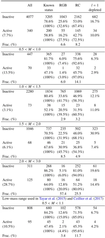
We retrieve the masses, radii and evolutionary status of the giants thanks to an asteroseismic analysis described in Sect. 2.4. By evolutionary status, we mean the RGB where stars burn H in shell around an inert He core, versus the RC, where He burn-ing occurs in the core. We distburn-inguish the red clump 1 (RC1) which consists of lower-mass stars (M . 2 M ) that reached the
clump after the He flash, from the red clump 2 (RC2) composed of intermediate-mass stars that smoothly kicked off the He com-bustion (e.g.,Mosser et al. 2014). We were able to measure the masses and radii of the 99.3% of RGs with detected oscillations, the evolutionary status of 3205 out of the 4077 inactive RGs, and 200 out of the 340 active RGs (including clear and ambiguous detection of rotational modulation). The inactive sample with a known status is composed of 33% of RGBs and 67% of RCs. The active sample is split in a similar way, with 28% of RGBs and 72% of RCs (see TableA.1).
Figure9shows the distributions of mass and radius for both the inactive and the active samples. A striking result is the very different mass distribution between the two samples (radius distributions are more similar). For the inactive RGs, the mass
distribution is consistent with previous reports based on CoRoT or Kepler observations (e.g.,Miglio et al. 2013). We note that it peaks at 1.3 M for RGBs and 1.15 M for RC, which could be
compatible with a significant mass loss during the late stages of the RGB phase. It also could be explained by the fact that we employed a unique asteroseismic scaling relation, whereas they should not be exactly calibrated in the same way for RGB and RC stars (Miglio et al. 2012;Khan et al. 2019). Regarding the active sample, we first note a general depletion of stars from 1.2 to 2 M . In particular, the RGB sample appears to be depleted
of low-mass stars and overpopulated of intermediate mass stars. The RC population is bimodal with a large group of RC1 stars on a narrow range (0.8–1.1 M ), and a large group of (mostly
RC2s) on a broad range (1.8–2.8 M ). Hereafter we often
distin-guish two groups by referring to low-mass RGBs and RCs (LM-RCs and LM-RGBs) with M ≤ 1.5 M , and high-mass RGBs
and RCs (HM-RGBs and HM-RCs) above.
3.3.2. Fraction of active RGs as a function of mass
If we consider the RGs with unknown evolutionary status to be equally distributed among the RGBs and RCs, we can estimate the absolute fraction of RGs in a given evolutionary status that display surface activity. We note them rRGB,act and rRC,act. For
instance, for the RGB group:
rRGB,act= NRGB,act ract,status NRGB,act ract,status + NRGB,inac rinac,status , (3)
where the fraction of active RGs with a known evolutionary status ract,status = Nact,status/Nact = 200/340 = 58.8%, and the
fraction of inactive RGs with a known status is rinac,status =
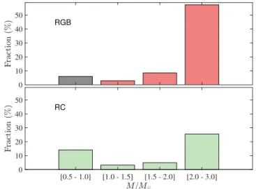
3205/4077 = 78.6% (see TableA.1). That way, 6.6% of RGBs and 8.2% of RCs are active. However, we observe a strong vari-ation of the occurrence of active RGs as both a function of mass and evolutionary status (Fig.10and TableA.1).
Let us first focus on the low mass part of the sample (M ≤ 1.1 M ) that was considered byTayar et al.(2015) andCeillier et al.(2017). Consistently with these two papers, we estimate the fraction of rapidly rotating RGs to be ract= 10.5%. Our study
brings new information thanks to the evolutionary status: it arises that only 3.4% of the RGBs are active, against 11.7% of the RCs. The fact that the fraction of low-mass active RGBs is two to three times smaller than that of active RCs is a strong indicator that the observed rotational modulation originates from an increased rotational rate happening on the RGB. Engulfment or merging of a stellar or substellar companion is a likely hypothesis (Simon & Drake 1989).
As regards stars with M ≥ 2 M , we find that about 60% of
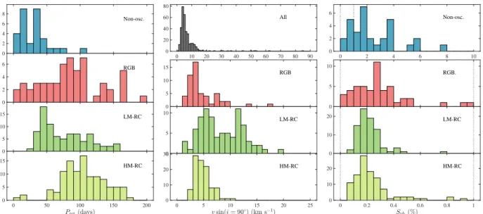
the RGBs and 25% of the RC2s are active. First of all, the smaller fraction of active RCs with respect to RGBs is compatible with loss of angular momentum starting during the RGB. Secondly, such a large rate of active RGs among intermediate-mass RGs was not reported byCeillier et al.(2017). As commented ear-lier, they likely missed this fraction of the sample because of catalog selection biases. At the same time, we confirm the con-clusions ofTayar & Pinsonneault(2018) who report that there is no large fraction of rapid rotators among intermediate mass RGs according to spectroscopic v sin i measurements if we stick to the 10 km s−1 criterion. Indeed, by combining the rotation periods with the asteroseismic radii, we compute the rotation velocities at equator v sin(i = 90◦). Figure11 (middle panel) shows v sin(i= 90◦) for the whole sample and for the individual
0.5 1 1.5 2 2.5 3 3.5 2 4 6 8 10 12 14 16 Inact., no evol Inact., RC Inact., RGB Act., no evol. Act., RC Act., RGB RGB inactive RGB active 0 0.05 0.1 0.15 0.2 0.25 RC inactive RC active 0.5 1 1.5 2 2.5 3 3.5 0 0.05 0.1 0.15 RGB inactive RGB active 0 0.1 0.2 0.3 0.4 RC inactive RC active 2 4 6 8 10 12 14 16 0 0.1 0.2 0.3 0.4
Fig. 9. Top panel: radius versus mass of the sample of 4465 stars. Red dots indicate the inactive RGBs, green the inactive RCs, and gray the inactive with unknown evolutionary status. Black squares indicate active RGBs, triangles active RCs and × signs active RGs with unknown evolutionary status. Panels b and c: distributions of masses and radii of the inactive and active RG samples as a function of stellar masses (top two panels) and radii (bottom two), according to their evolution-ary stages. Empty histograms correspond with the inactive samples, red with the active RGBs, and green with active RCs.
evolutionary stages. Regarding the HM-RC stars, only ≈4% show v sin(i= 90◦) ≥ 10 km s−1.
Interestingly, we notice that the only group that shows a sig-nificant fraction (≈37%) of stars with v sin(i= 90◦) ≥ 10 km s−1 is the LM-RC group, which is suspected to have engulfed a stel-lar or substelstel-lar companion. Finally, by considering all of our RGs with detected rotational modulation and oscillations, the fraction of stars with v sin(i = 90◦) ≥ 10 km s−1is about 17%.
RGB
off off off off
0 10 20 30 40 50 RC [0.5 - 1.0] [1.0 - 1.5] [1.5 - 2.0] [2.0 - 3.0] 0 10 20 30 40 50
Fig. 10.Bar graph showing the fraction of active RGs among the RGB and RC groups as a function of mass. For each mass bin, the estimate of the fraction of active stars is extracted from the number of active stars, the number of inactive stars, and the ratio of stars with a known
evolutionary status as explained in Sect.3.3.2(Eq. (3)). All the numbers
used to produce this graph are displayed in TableA.1. For RGBs with
M ∈[0.5, 1.0] R , the bar is gray because it relies on a very small sample
(1 active and 27 inactive RGBs, see TableA.1), and is not statistically
secure.
By assuming that all of the inactive RGs have v sin i < 10 km s−1,
it means that 1.4% of our whole sample show v sin(i = 90◦) ≥ 10 km s−1, which is a little less than the 2% reported byCarlberg et al.(2011).
3.3.3. Rotation rate versus activity
Firstly, we observe a strong difference of the photometric activ-ity index Sph between the nonoscillating (almost all close
bina-ries) and the oscillating active RGs (mostly single RGs) from our sample. From Figs. 11 and 12, the nonoscillating RGs show values of Sph from about 1 to 10%, whereas all of the
others display maximum values an order of magnitude lower (0.1 to 1%). As shown by Gaulme et al. (2014, 2016), and
Benbakoura et al. (2020), the nonoscillating RGs in EBs are almost all both synchronized and circularized. The few non-locked systems are pseudo-synchronized. It means that the rota-tion rate is not the only factor driving the amplitude of rotarota-tional modulation and oscillations: tidal locking causes in a way or another more photometric contrast. Understanding that aspect goes beyond the scope of this paper.
Regarding the single active RGs, our results show that rota-tional modulation appears at rotation rates much smaller than the “fast rotation” threshold that is usually considered. We indeed detect rotational modulation for RGs with v sin i ≥ 2 km s−1. To put this result in its usual theoretical context (e.g., Noyes et al. 1984;Wright et al. 2011), we consider the generation of magnetic field in the frame of the turbulent dynamo scenario (e.g.,Charbonneau 2014). In such a scenario, the efficiency of the magnetic field generation is characterized by the Rossby number Ro = Prot/τc. The efficient dynamo regime, and hence
surface magnetic fields and spots, is associated with Ro ≤ 1. We thus need an estimate of the convective turnover timescale τcfor
the stars in our sample.
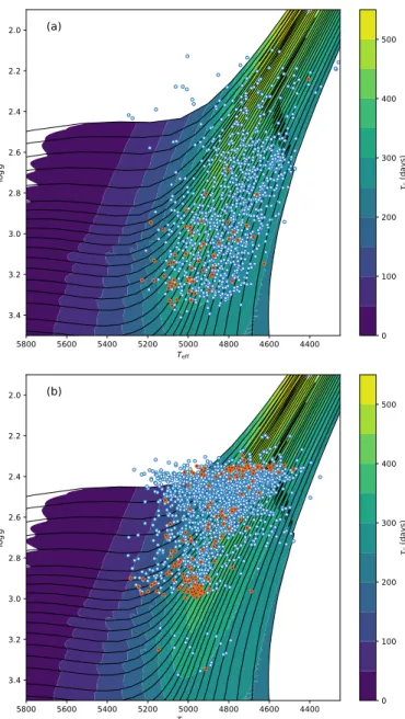
In Fig. 13, isolevels of τc are overplotted with the data;
evolutionary tracks are also shown for reference. We use the τc extracted from the stellar evolution tracks from the YaPSI
Non-osc. 0 50 100 150 200 0 2 4 6 8 RGB 0 50 100 150 200 0 2 4 6 LM-RC 0 50 100 150 200 0 5 10 15 HM-RC 0 50 100 150 200 0 5 10 15 All 0 10 20 30 40 50 60 70 80 90 0 20 40 60 80 RGB 0 5 10 15 20 25 0 5 10 15 LM-RC 0 5 10 15 20 25 0 5 10 HM-RC 0 5 10 15 20 25 0 10 20 30 Non-osc. 0 2 4 6 8 10 0 2 4 6 RGB. 0 0.2 0.4 0.6 0.8 1 0 5 10 LM-RC 0 0.2 0.4 0.6 0.8 1 0 10 20 HM-RC 0 0.2 0.4 0.6 0.8 1 0 10 20
Fig. 11.Left panel: distribution of the measured rotation periods expressed in days. Colors indicates RC (green), RGB (red), and nonoscillating
(blue) targets. Middle panel: equatorial velocities of the active RGs, that is v sin(i= 90◦
). Top subpanel: v sin(i= 90◦
) for the whole active sample
where oscillations are detected. Next subpanels: same for RGB, LM-RC, and HM-RC, by considering only the range [0, 25] km s−1with bins of
1 km s−1. Right panel: distribution of the light-curve standard deviations of the same groups as on left panel, expressed in percent. The dotted lines
indicate the range [0.1, 1]%.
0 20 40 60 80 100 120 140 160 180 200 0.02 0.1 0.2 1 5 10 No osc. RGB LM-RC HM-RC
Fig. 12.Photometric index Sph(percent) as a function of rotation period
Prot (days) for the RGs with rotational modulation. The photometric
index Sphis plotted in log scale, Protin linear scale. Blue squares
indi-cate the nonoscillating RGs, red disks the RGBs, darker green upward-pointing triangles the low-mass RCs, and lighter downward-upward-pointing triangles high-mass RCs. The markers that display black edges are con-firmed spectroscopic binaries. Black dots indicate RV stable RGs. The
gray background reflects the distribution of Sphof the inactive stars (the
darker, the higher).
database (Spada et al. 2017). It should be noted that the values of τcshown in the Figure were calculated using the mixing-length
treatment of convection (seeSpada et al. 2017for details), which is adequate to provide an estimate to the leading order.
From Fig.13, it is apparent that all of our ≈4500 RGs could be active if their rotational periods were less than about 250 days. In this Teff–log g diagram (Kiel diagram), active and inactive
RGs overlap, which tends to indicate that the inactive stars rotate slower, likely with rotation periods longer than about 250 days. Among the RGB stars (panel a) the active subsample is concen-trated around the region of the first dredge-up, that is, near the
base of the RGB. For the RC stars (panel b of Fig.13), two dis-tinct subpopulations of active stars exist, roughly corresponding to the low-mass and the intermediate mass regimes. The former have log g ≈ 2.4, while the latter have larger surface gravity and are distributed with approximately the same scatter in log g and Teff. Both characteristics are consistent with the predictions of
classic stellar evolution theory for the RC and the secondary RC, respectively (see, e.g.,Girardi 2016).
This result also needs be compared with spectro-polarimetric observations of magnetic RGs (e.g.,Aurière et al. 2011,2015;
Konstantinova-Antova et al. 2012,2013) and the subsequent the-oretical work byCharbonnel et al.(2017).Aurière et al.(2015) describes spectropolarimetric observations of a sample of 48 magnetically active RGs, and report clear detection of magnetic fields in 29 stars. Rotation periods are known for most of these stars, and range from about 6 to 600 days. They observe that the magnetic RGs are distributed along a so-called “magnetic strip” in the Hertzsprung–Russell diagram, which is a region where τc is maximum. Such a condition is met during the first
dredge up phase at the bottom of the RGB, as well as for RC stars. This result is fully compatible with ours. The only notable difference with their results is that they identify a correlation between the chromospheric activity and the stellar rotation peri-ods. We do not find such a trend between Sphand Prot(Fig.12).
This could be due to the fact that their sample spans a broader range of periods (most of our single RGs show periods from 40 to 170 days). Moreover, the chromospheric index Sindexand the
Zeeman measurements are not sensitive to the stellar inclination contrarily to Sph, which makes trends clearer to appear.
Aurière et al.(2015) also identify a few outliers that could be descendent of magnetic Ap stars (e.g.,Aurière et al. 2011;
Borisova et al. 2016;Tsvetkova et al. 2019). These outliers are characterized by an enhanced chromospheric activity Sindexwith
respect to their peers with similar rotation periods. We identify one star among our single RGs with strong activity that could match this description. KIC 5430224 has Sph = 1.1% but is
RV stable with no particularly fast rotation (Prot ≈ 55 days).
4400 4600 4800 5000 5200 5400 5600 5800 Teff 2.0 2.2 2.4 2.6 2.8 3.0 3.2 3.4 lo g g (a) 0 100 200 300 400 500 τc ( da ys) 4400 4600 4800 5000 5200 5400 5600 5800 Teff 2.0 2.2 2.4 2.6 2.8 3.0 3.2 3.4 lo g g (b) 0 100 200 300 400 500 τc ( da ys)
Fig. 13.Stars with detected oscillations in our sample compared with stellar evolution tracks and isocontours of the convective turnover
timescale in the (Teff, log g) plane. Panel a: RGB stars; panel b: RC
stars; stars with and without detected rotational modulation (i.e., “mag-netic activity”) are plotted in red and blue, respectively.
KIC 8160175 (Sph = 2.6%) seems to be caused by
contamina-tion of a nearby star (see AppendixB) and cannot be counted as a possible Ap descendent.
4. Conclusions
The original objective of this work was to determine what frac-tion of RGs shows activity (rotafrac-tional modulafrac-tion), and under-stand its origin. One of the underlying questions was the role of close binarity in this population, standing upon the fact that RGs in close binary systems (Porb. 200 days) have been observed to
display strong rotational modulation.
To avoid as much as possible being influenced by obser-vational biases, we carefully selected a subsample of the RGs observed by the Kepler satellite during its original four-year mis-sion. This sample was picked from theBerger et al.(2018) stellar
classification of the Kepler field based on the Gaia DR2. From their sample of RGs, we selected the targets whose light curves should not be limited by the photon noise, meaning that the oscil-lations of a regular RG should be detectable. This led us to con-sider the brightest stars (mKep ≤ 12.5 mag) that were observed
the longest (more than 3 years). We added a cut on radii, to make sure that the oscillation range would fall between 15 µHz and the sampling cut-off (Nyquist frequency) at ≈283 µHz. The final sample is composed of 4465 RG stars (Fig.14).
Our first result is the clear detection of SL oscillations in 99.3% of the sample, which is a much larger fraction than reported in previous studies (e.g.,Stello et al. 2013;Hon et al. 2019). We explain this mainly thanks to the fact that our spe-cial sample is not affected by photon noise for searching for RG oscillations. We also paid much attention to search for oscilla-tions in low S/N conditions. The second important finding is that between 6.7% (only clear detection) and 8.3% (including low S/N detection) of RGs display rotational modulation, which is much larger than reported by previous studies, in particular by Ceillier et al.(2017). We also clearly show that the active RGs present oscillations with lower amplitudes with respect to the inactive sample (Fig.7). This latter fact – increased activ-ity leads to lower modes – was previously observed for MS stars (e.g.,Chaplin et al. 2011;Mathur et al. 2019), but also for RGs in close multiple systems (e.g.,Derekas et al. 2011;Gaulme et al. 2014;Benbakoura et al. 2020).
From high-resolution spectroscopic observations specially conducted with the échelle spectrometer of the 3.5 m ARC tele-scope, as well as public SDSS/APOGEE observations, we could determine the role of close binarity in the origin of the active RGs. It appears that among the 30 nonoscillating active RGs, 26 are clear SBs, one lacks in statistically significant RV varia-tions, and another three are possible SBs. This means that almost all of the nonoscillating RGs belong to close binary systems. Among the rest of the sample, that is, the active RGs with par-tially suppressed but detectable oscillations, the fraction of close binaries is still significantly larger than in among the inactive ones. We count about 15% of SBs whereas we identify only 1% in a test sample composed of inactive RGs. This also means that a large majority of active RGs with detectable oscillations does not belong to close SBs.
We shed light on the origin of the active single RGs by ana-lyzing their distributions in terms of physical properties (mass, radius) and evolutionary status (RGB, RC). It arises that most of the active RGs fall into two distict groups: a low-mass (M ≤ 1.5 M ) and an intermediate-mass range (1.8 ≤ M ≤ 2.8 M ).
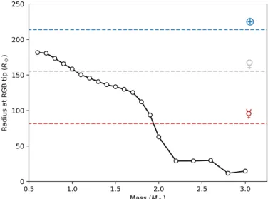
The low-mass part of the active RGs is mostly composed of stars on the RC: about 3% of the RGBs are active while about 12% of the RCs are active. This means that a fraction of the RGs in that mass range gains angular momentum between the RGB and the RC. This observation favors the scenarios of planet engulfment or merging with small stellar objects. Indeed, low-mass stars ignite Helium after the He flash, and present radii up to ∼200 R at the tip
of the RGB (Fig.15), and may swallow planets, converting their orbital momentum into spin and friction loss. Another option is a stellar engulfment. Highly eccentric systems (0.3 < e < 0.8) as those composing the heartbeat systems (e.g.,Beck et al. 2014;
Kuszlewicz et al. 2019) are typically composed of a Sun-mass star and a much smaller companion (0.2 M ). Near the tip of the RGB,
the most massive star has a radius larger than the periastron dis-tance and thus merges with the companion.
If this scenario of planet or stellar engulfment is true, it is inter-esting to notice that it regards a relatively narrow mass range. This can be qualitatively explained by three factors. Firstly, since more
4465 red giant stars
(4077 inac2ve + 340 ac2ve w. osc. + 30 ac2ve w/o osc. + 18 with inconsistent M,R) 1043 RGB (25.6%) 872 Unknown (21.4%) 2162 RC (53.0%) 55 RGB (14.9%) 145 RC (39.2%) 140 Unknown (37.8%) 30 Non-oscilla2ng (8.1%) No rota2onal modula2on Regular oscilla2ons 4077 (91.3%) Rota2onal modula2on Suppressed oscilla2ons 370 (8.3%)Fig. 14.Diagram that summarizes the sample we analyze in this paper. The hatched areas indicate the fraction of spectroscopic binaries among a given population. They represent about 85% of the nonoscillating active RGs, 15% of the active RGs with partially suppressed oscilla-tions, and 2% of the inactive RGs according to our spectroscopic sam-ple. We note that the percentages in the active sample slightly differ
from those reported in TableA.1because they refer to the 370 active
stars (with and without detected oscillations) in the present diagram,
whereas they refer to the 340 RGs with oscillations in TableA.1.
massive stars (M ≥ 2 M ) do not reach the clump through the He
flash, their radii do not exceed ≈20 R , so they are less
suscepti-ble to engulf planets. Moreover, because they are more massive, they gain relatively less angular momentum by swallowing plan-ets than less massive stars. Lastly, the orbital angular momentum of close-in planets increases as a function of the semi-major axis, and thus is less efficient with a close planet with respect to a planet like Venus, orbiting at 150 R .
As regards intermediate-mass stars, we observe that a large fraction of the RGBs is active (over 50% when M ≥ 2 M ),
and a large but reduced fraction of active RCs (about 25%). In opposition to the low-mass range, this observation implies that intermediate-mass stars tend to loose angular momentum between the RGB and the clump. Both the fraction of the active RGB in this mass range and the fact that they loose momentum between the RGB and the RC are compatible with the expected scenario for intermediate-mass stars. They do not loose angular momentum during the MS, thus still spin fast on the RGB, and a little less once on the clump. However, the values are still in con-trast with recent theoretical studies (e.g.,Tayar & Pinsonneault 2018). From the observed distribution of rotation rates of A and B-type MS stars, about half of the RGs are expected to display vsin i ≥ 10 km s−1(e.g., Ceillier et al. 2017). From our astero-seismic radii and photometric rotation periods, we measure that only about 4% of the active intermediate-mass RGs display such a rapid rotation, that is about 2% of that mass range by including the inactive ones. This reinforces previous reports of an uniden-tified sink of angular momentum after the MS.
Regarding the connection between the emergence of surface activity, we observe that RGs with v sin i ≥ 2 km s−1show
rota-tional modulation. This is actually not surprising when we com-pare the rotation periods of the active RGs with the convective turnover time τc. In a turbulent dynamo scenario, the generation
of magnetic fields starts being efficient if the rotation period is lower than τc. All the active RGs meet these conditions (Fig.13).
0.5 1.0 1.5 2.0 2.5 3.0 Mass (M⊙⊙ 0 50 100 150 200 250 R ad iu s at R G B ti p (R⊙ ⊙
☿
♀
☿
Fig. 15.Stellar radius at the tip of the red giant branch as a function of mass as predicted by the stellar models used in this work. No mass loss was considered during the RGB phase. The semimajor axes of the current orbits of Mercury, Venus, and Earth are also marked for com-parison.
A correlated interesting fact is that the active RGs that belong to binary systems and that do not display oscillations show a pho-tometric activity index Sph about an order of magnitude larger
than single active RGs. We could explain this by the fact that the nonoscillating active RGs have rotation periods shorter in average than the single active RGs. However, we observe that single RGs with rotation periods between 30 and 80 days still show an Sph about ten times less than the RGs in SBs with the
same periods. This implies that tidal locking somehow leads to larger magnetic fields, and also a more efficient oscillation sup-pression. Investigating that aspect will be part of future works. Last,Mathur et al.(2019) report that MS stars with Sph≥ 0.2%
never show SL oscillations. We note that this threshold is not the same for RGs, as we detect oscillations up to levels of about Sph≈ 1%.
Further developments of this project will cover several aspects. Firstly, complementary high-resolution measurements of the identified SBs will help to better characterize the types of systems that compose the population of close binaries with an RG. In particular, we can infer the mass ratio for the SB2s. We will also study the possibility of leading infrared interfer-ometric measurements to resolve the brightest and closest sys-tems and retrieve the mass and radii of the individual compo-nents. As regards the other topics covered in this work, we will perform a detailed analysis of the HR spectra and look for chem-ical peculiarities of the LM-RC stars, in order to spot possi-ble signatures of merging history. Among possipossi-ble tracers, we will especially monitor the Lithium absorption line as suggested by Soares-Furtado et al. (2020), for example, which we have already identified for a handful of targets (see TableB.1). As regards the fast rotating intermediate-mass RGs, we will inves-tigate, in more details, the analysis of mixed modes to estimate the rotation rate of the core, to measure the evolution of angular momentum between the RGB and RC phases.
Acknowledgements. P. Gaulme, F. Spada, and C. Damiani acknowledge fund-ing from the German Aerospace Center (Deutsches Zentrum für Luft- und Raum-fahrt) under PLATO Data Center grant 50OO1501. M. Vrard was supported by FCT – Fundação para a Ciência e a Tecnologia through national funds and