Deciphering records of geomagnetic reversals

HAL Id: insu-02400962

https://hal-insu.archives-ouvertes.fr/insu-02400962

Submitted on 9 Dec 2019

HAL is a multi-disciplinary open access

archive for the deposit and dissemination of

sci-entific research documents, whether they are

pub-lished or not. The documents may come from

teaching and research institutions in France or

abroad, or from public or private research centers.

L’archive ouverte pluridisciplinaire HAL, est

destinée au dépôt et à la diffusion de documents

scientifiques de niveau recherche, publiés ou non,

émanant des établissements d’enseignement et de

recherche français ou étrangers, des laboratoires

publics ou privés.

Jean-Pierre Valet, Alexandre Fournier

To cite this version:

Jean-Pierre Valet, Alexandre Fournier. Deciphering records of geomagnetic reversals. Reviews of

Geophysics, American Geophysical Union, 2016, �10.1002/2015RG000506�. �insu-02400962�

Deciphering records of geomagnetic reversals

Jean-Pierre Valet1and Alexandre Fournier1

1

Institut de Physique du Globe de Paris, Sorbonne Paris Cité, Université Paris Diderot, UMR 7154 CNRS, Paris, France

Abstract

Polarity reversals of the geomagneticfield are a major feature of the Earth’s dynamo. Questions remain regarding the dynamical processes that give rise to reversals and the properties of the geomagnetic field during a polarity transition. A large number of paleomagnetic reversal records have been acquired during the past 50 years in order to better constrain the structure and geometry of the transitionalfield. In addition, over the past two decades, numerical dynamo simulations have also provided insights into the reversal mechanism. Yet despite the large paleomagnetic database, controversial interpretations of records of the transitionalfield persist; they result from two characteristics inherent to all reversals, both of which are detrimental to an ambiguous analysis. On the one hand, the reversal process is rapid and requires adequate temporal resolution. On the other hand, weakfield intensities during a reversal can affect the fidelity of magnetic recording in sedimentary records. This paper is aimed at reviewing critically the main reversal features derived from paleomagnetic records and at analyzing some of these features in light of numerical simulations. We discuss in detail thefidelity of the signal extracted from paleomagnetic records and pay special attention to their resolution with respect to the timing and mechanisms involved in the magnetization process. Records from marine sediments dominate the database. They give rise to transitional field models that often lead to overinterpret the data. Consequently, we attempt to separate robust results (and their subsequent interpretations) from those that do not stand on a strong observational footing. Finally, we discuss new avenues that should favor progress to better characterize and understand transitional field behavior.

1. Introduction

Geomagnetic reversals are an extreme manifestation of the variability of the geomagneticfield created and sustained by dynamo action in Earth’s core. This variability spans a vast range of time scales, from days to millions of years. Composite power spectra of dipole fluctuations constructed from observations [Constable and Johnson, 2005] and numerical dynamo simulations [Olson et al., 2012] point to an intermedi-ate frequency band with periods from a few centuries to a few tens of kiloyears, where, according to Olson et al. [2012], the energy density increases with the period in an almost quadratic fashion; reversals (and excursions, i.e., failed attempts at reversal) lie within that transitional band (that of paleosecular variation). No obvious separation of excursional to reversing behavior exists, and the question remains whether reversals reflect core processes that are different from those at work behind regular paleosecular variation. In this review, our primary goal is to outline the constraints that current (and future) observations may help to place on these processes, by means of a detailed description of the so-called transitionalfield, i.e., the global geomagneticfield one would map out during a reversal. Good knowledge of transitional field beha-vior is also key to predicting how the Earth system (and, in particular, the magnetosphere) would evolve in the event of a reversal (see, e. g., the discussion by Constable and Korte [2006] and the review by Glassmeier and Vogt [2010]).

Thefirst records of geomagnetic reversals were published more than 50 years ago [Van Zijl et al., 1962; Momose, 1963]. Since then an increasing number of records have been obtained from rock types with diverse physicochemical processes of formation and magnetization. Most studies have dealt with sediments, no more than two dozens from lavaflows, and three records from intrusions [Dodson et al., 1978]. In most cases, identification of reversals relies on detailed magnetostratigraphic profiles for sediments and on radiometric ages for lavaflows. Considerable progress has been achieved over the past 20 years by tuning carbonate variation in sedimentary sequences to Earth’s orbital variations with a precision better than 20 kyr [Imbrie et al., 1992]. However, this time span exceeds the duration of reversals. It is, therefore, difficult to determine rapid geomagnetic variations with adequate temporal precision. These differences are amplified by weak transitionalfields that contribute to increase recording complexities.

Reviews of Geophysics

REVIEW ARTICLE

10.1002/2015RG000506

Key Points:

• We examine and assess an updated database of geomagnetic reversal records

• We discuss robust and controversial features of the transitionalfield • Future work should involve

millimeter-size specimens and physics-based models

Correspondence to:

J.-P. Valet, valet@ipgp.fr

Citation:

Valet, J.-P., and A. Fournier (2016), Deciphering records of geomagnetic reversals, Rev. Geophys., 54, 410–446, doi:10.1002/2015RG000506.

Received 10 OCT 2015 Accepted 17 MAR 2016

Accepted article online 24 MAR 2016 Published online 17 MAY 2016

©2016. The Authors.

This is an open access article under the terms of the Creative Commons Attribution-NonCommercial-NoDerivs License, which permits use and distri-bution in any medium, provided the original work is properly cited, the use is non-commercial and no modifications or adaptations are made.

Like any scientific topic, our knowledge about field reversals has been acquired through several steps. A first important objective was to determine whether the field would maintain a dipolar character when reversing. Early studies [Creer and Ispir, 1970] proposed that thefield had retained dipolar configurations during seven polarity reversals recorded at widely separated sites. The motion of the pole through the Indian Ocean was simulated by a model of three dipoles that was rapidly discarded with accumulation of new results, mostly from sediments. The dipolar nature of the transition was also questioned by thefirst measurements of absolute paleointensity which showed that polarity changes are accompanied systema-tically by lowfield values [van Zijl et al., 1962; Momose, 1963; Coe, 1967; Lawley, 1970; Larson et al., 1971; Niitsuma, 1971; Dagley and Wilson, 1971]. These observations were reinforced by the dominance of low magnetization intensities associated with transitional lava flows [Kristjansson and McDougall, 1982]. Thefirst compilation of volcanic records led Dagley and Lawley [1974] to favor a nondipolar transitional field. By then a succession of models had been proposed and tested against an increasing number of paleomagnetic data.

Knowledge offield geometry during polarity reversals remains limited due to the difficulty of acquiring well-documented records of the same transition from widely distributed locations, particularly from the Southern Hemisphere which remains relatively depleted of data. Despite advances in determining successivefield directions, along with relative and absolute paleointensity changes during transitions, interpretations are hampered frequently by relatively poor knowledge of the processes involved in magnetization acquisition, especially for sediments, and by the absence of a detailed chronology for lavaflow sequences.

The last reversal (Matuyama-Brunhes, M-B) has been the focus of much attention, because this is thefirst major event that can be recognized in marine sediment cores. The successive positions of the virtual geo-magnetic pole (VGP)—the apparent location of the pole assuming an axial geocentric dipole field—that define the VGP path have been commonly used to infer features of the transitional field. The first five pub-lished M-B records showed some tendency of VGP paths to lie near the longitude of their sampling site. Hoffman and Fuller [1978] concluded that the transitionalfield was predominantly controlled by degree 2 or 3 zonal harmonics and, therefore, it was axisymmetric but not dipolar. As more detailed records of the last reversal and other events became available, these models could not be defended any more. It was then con-sidered that thefield was neither axisymmetric [Hoffman, 1979; Fuller et al., 1979; Valet et al., 1988a; Prévot, 1977; Prévot et al., 1985; Clement and Kent, 1984] nor dipolar but likely controlled by nonzonal harmonics of low degree [Hoffman, 1984]. Unfortunately, in this case a large distribution of sites that record the same reversal is needed to determine the exact nature of the harmonic content. Studies of geomagnetic reversals turned toward a different prospect in the early 1990s with the aim of investigating the imprint of the lower mantle on the geomagneticfield [Gubbins, 1994].

Most inferences about the reversingfield are controversial. We attempt to approach these topics from a different angle than previous reviews on reversals [Clement and Constable, 1991; Bogue and Merrill, 1992; Jacobs, 1994; Roberts, 1995; Merrill and McFadden, 1999; Constable, 2003; Valet and Herrero-Bervera, 2007; Amit et al., 2010] and present here a critical review on the subject. We discuss the resolution and precision that can be expected to describe the transitionalfield. Many observations remain controversial due to limited constraints on magnetization signals and their temporal sampling. Using the last reversal as a detailed case study and evaluating the published database, we conclude that attempts at describing thefirst terms of the harmonic content of the transitionalfield remain premature. Another issue concerns the longitudinal prefer-ence of VGP paths during different reversals and/or the presprefer-ence of VGP clusters that could reflect heteroge-neous heatflux at the core-mantle boundary, but they could also be generated by rock magnetic or sampling artifacts. Finally, the magneticfield is a vector and studies of paleointensity are essential to document the transitionalfield. Few volcanic records provide successful paleointensity determinations, but those that do contain some coherent features. Dipolefield intensity evolutions across various reversals from sedimentary records reveal interesting but controversial features. Wefinally report on promising avenues opened by new and supplementary techniques.

Parallel to data acquisition, activity has been invested in developing numerical dynamo models and analyz-ing their output (see the recent short review by Glatzmaier and Coe [2015]). We can now attempt to gain additional insights into reversal features revealed by paleomagnetic records with respect to those produced by numerical simulations.

2. Resolution of Paleomagnetic Records

In order to assess the role played by nondipolar components during transitions, we need to consider typical characteristic times of the recent nondipolefield, of which we have an arguably reasonable knowledge. The characteristic time scales of secular variation can be estimated from spatial power spectra of the mainfield and of its secular variation. These time scales represent statistically the time it would take for the energy of thefield at spherical harmonic degree n to be completely renewed [Hulot and Le Mouël, 1994]. The time scales of the nondipolefield (n > 1) are compatible with an inverse linear law of the form τ_n=τ_sv/n with a master coefficient, the secular variation constant τsv, of the order of 500 years [Lhuillier et al., 2011a], when estimated

based on the historical geomagneticfield model gufm1 [Jackson et al., 2000]. Therefore, over a period of approximately 1 kyr, the nondipolefield will be reorganized substantially. In addition, τnvalues for low n,

which can be computed directly using time-averaged spectra of thefield and secular variation of the regularized holocenefield model CALS10k.1b [Korte et al., 2011] range from 458 years (n = 2) to 155 years (n = 6). We take from thesefigures that proper description of nondipole field evolution requires a temporal resolution that should be less than a millennium.

The concept of transitional directions does not have any clear theoretical meaning. It is convenient to con-sider that a direction is transitional when it exceeds the normal range of secular variation. However, if we assume that reversals belong to a continuum of geomagnetic changes covering the characteristic time scales for secular variation and excursions, this definition is not meaningful since directions pointing far away from the direction of the axial dipolefield at the site can also be generated by secular variation in weak field. Transitional directions are usually defined from VGP latitudes that are either lower than 60° or 45° (60° is commonly used for volcanics while 45° is more often adopted for sediments where inclination shallowing is common). When a detailed record of paleosecular variation accompanies a reversal, it is convenient to refer to the maximum change in amplitude reached during the surrounding intervals of stable polarity. Another approach has been proposed by Vandamme [1994] that takes into account the limit of VGP scatter around the mean pole position. This technique requires good knowledge of the localfield during periods of full polarity surrounding the transition. We must also be aware that the criteria used to define reversal boundaries rely on directions and not on the full vector. The localfield direction is constrained by the axial dipole inten-sity and the remaining nonaxial dipolefield (i.e., the field without the axial dipole, frequently referred to as the nonaxial dipolefield, NAD). Depending on site location, a large axial dipole decrease may not always be accompanied by a significant deviation of the local field direction, despite being related to transitional processes. Therefore, in such cases paleointensity determinations are crucial.

2.1. The Convoluted Signal of Magnetic Remanence in Sediments

The continuous character of sediment records is attractive when studying short geomagnetic events like reversals, but this advantage is counterbalanced by their weak magnetization. For this reason, development of thefirst cryogenic magnetometers in the 1970s enabled accurate measurement of weakly magnetized sediment samples, which opened the way to studies of polarity transitions and secular variation. Typical 8 cm3single samples used for magnetic measurements average thefield over the time required for deposi-tion of 2 cm of sediment. This constraint alone makes it impossible to obtain clues about nondipolefield changes recorded at deposition rates lower than 10 cm/kyr if one wishes to have a 200 year resolution. Smaller subsamples can be used, but we then have the delicate task of sampling thin slices of sediment without introducing disturbances, a problem that is amplified by the weak magnetization of transitional samples. Resolution becomes even poorer when analyzing long continuous sections of sediment (refered to as U-channels) since the wide response curves of the magnetometers (i.e., the sediment thickness inte-grated in each measurement) generate additional smoothing [Nagy and Valet, 1993; Weeks et al., 1993]. Similar conclusions were reached for records of geomagnetic excursions by Roberts and Winklhofer [2004]. Further complexity arises from the magnetization process itself. There is strong evidence that bioturbation (i.e., mixing of sediment by biological activity) introduces an offset between the position of the actual reversal and its record within the sediment. Under such conditions, it is difficult to argue that magnetization lock-in occurs immediately below the bioturbated layer. There is an ongoing debate regarding the way sedimentary magnetization is acquired. Only a small portion of magnetic grains is oriented by thefield. A key question is to determine whether this is caused by integration of magnetic grains within sedimentaryflocs that impede their alignment with thefield and if such aggregates form in the water column, at the sediment-water

interface, or below the bioturbated layer [Katari and Bloxham, 2001; Tauxe et al., 2006; Shcherbakov and Sycheva, 2010; Spassov and Valet, 2012; Roberts et al., 2013]. The most stable part of the magnetization carried byfine particles is oriented during periods of full polarity, in the presence of stronger fields than during reversals. This raises the question of whether these grains can be oriented when thefield is 1 order of magnitude weaker.

Magnetization lock-in is argued to result from a progressive decrease in sediment water content [Irving and Major, 1964; Kent, 1973]. We thus suspect that magnetization is acquired over at least a 10–15 cm deep interval [e.g., Channell and Guyodo, 2004; Liu et al., 2008; Suganuma et al., 2011; Ménabréaz et al., 2014]. Assuming a deposition rate of 6 cm/ka and a 12 cm deep interval for lock-in, the sediment magnetization will integratefield changes over a 2 kyr long period. Even with a 6 cm lock-in zone, the signal is smeared over a 1 kyr period, which is too long to properly document variations of nondipolefield components.

2.2. Limits Imposed by Sediment Depositional Processes

The effect of deposition rate and lock-in depth on the resolution of sedimentary paleomagnetic records can be investigated by referring to the historical and archeologicalfield. The most complete record of paleosecu-lar variation for the past 5 ka has been obtained from the big island of Hawaii [Hagstrum and Champion, 1995]. Each unit has a14C age with an averaged uncertainty of 120 years. In parallel, a highly detailed sedi-mentary record has been obtained from nearby Lake Waiau from the summit of Mauna Kea [Peng and King, 1992]. This unique situation allows comparison of these two independent detailed and accurate data sets offield changes during the past 5 ka. The two inclination patterns in Figure 1a are similar, except for intervals that seem to be offset from each other likely because of dating inaccuracies. A striking observation is that all short-termfluctuations present in the lava record appear to be smoothed out in the sedimentary record. The variations present in the volcanic data do not result from errors in sample orientation or from tilt-ing of lavaflows. Their presence cannot be linked to the magnetization process and, therefore, reflect local geomagnetic changes. We have investigated the time window required to smear out the variations in order to reconcile the records. If we simulate a marine record characterized by the same deposition rate of 43 cm/kyr as at Lake Waiau and use the volcanic data as the initialfield changes, we find that a 200 year inte-gration time is required to match at best both records (Figure 1b). This corresponds to an 8–10 cm lock-in depth, which is not large but significant enough and confirms that even with rapid deposition rates sediment magnetization undergoes low-passfiltering.

The same Hawaiian volcanic sequence provides a partial description offield changes, but they are detailed enough to allow investigation of the transformation of this signal by magnetization processes in sediments. We have, thus, simulated VGP successions that would be recorded by sedimentary sequences with deposi-tion rates of 10 cm/kyr, 4 cm/kyr, and 2.5 cm/kyr. Note that the lower two values are typical of marine sequences that have been studied extensively to obtain records of polarity transitions and that there are few studied sedimentary records with deposition rates as high as 10 cm/kyr. Each data point in Figure 1c represents a VGP obtained from a 2.5 cm long cylindrical sample. The VGP positions are different from their initial configuration even for records with rapid deposition rates. Most low-latitude data points have disap-peared and the longitudinal distribution of VGPs is different. We also investigated the effect of smearing caused by postdepositional reorientation over a 10 cm deep layer with a 10 cm/kyr deposition rate. In this situation, which is likely more realistic, the results depict a smooth succession of VGPs across 180° of longi-tude. This recording differs significantly from the actual field changes.

We can explore further the consequences of the low resolution that is inherent to sedimentary paleomag-netic signals by relying on CALS10k.1b, geomagpaleomag-neticfield model [Korte et al., 2011]. We have simulated a complete reversal by decreasing the axial dipole intensity until it reaches zero and subsequently recovers with the opposite sign, over a 10,000 year period. From this succession offield changes, we computed equivalent sedimentary records for various deposition rates. In Figure 1d we show the typical case of a rever-sal simulated at the same location as the 16.7 Ma Steens Mountain record from Oregon [Jarboe et al., 2011], which is also shown for comparison. The VGP path derived from the model is less complex than the Steens Mountain paleomagnetic record, likely because CALS10k.1b is built from the current archeomagnetic and sedimentary database [Korte et al., 2011] and thus fails to describe in detail the local and rapidfield changes that could exist during a reversal. Transitional VGPs obtained for a sequence with a deposition rate of 4 cm/kyr, which is typical of most sedimentary records, have a much smoother configuration than those of

the initialfield. Additional smearing caused by postdepositional reorientation of magnetic grains further increases the tendency of transitional VGPs to be distributed along the same longitude in contrast to the 200° longitudinal crossing in the initial path.

2.3. Is the Weak Magnetization of Sediments Appropriate for Reversal Studies?

Time averaging inherent to the recorded remanent magnetization of sediments may generate another pro-blem regarding definition of the characteristic component of magnetization that is isolated after demagne-tization. In Figure 2 we show demagnetization diagrams for samples from two sediment cores in the Indian and North Atlantic Oceans, respectively. Outside the transition zones the characteristic components are well defined and decrease linearly to the origin of the demagnetization diagrams. Samples from the transition

Figure 2. Typical demagnetization diagrams for samples from cores MD95-2016 and MD90-949 that recorded the last reversal. Diagrams in the middle panel correspond to transitional samples. Note that the large dispersion of successive directions prevents determination of a clear characteristic magnetization component. This behavior is encountered in most, if not all, reversal studies from sediments with deposition rates lower than 5 cm/kyr. It is most likely caused by overlapping of different directions.

Figure 1. (a) Inclination changes recorded by volcanic and sedimentary sequences at the same location (big island of Hawaii) for the same time period. (b) Same as Figure 1a after time averaging the volcanic data within successive 200 year long windows. (c) Stereographic projections of VGPs that correspond to the signal in Figure 1a recorded by sediments with different deposition rates; VGPs are plotted on the right-hand side. The top right plot illustrates the effect of pro-gressive magnetization locking over a 10 cm interval. (d) (top) Volcanic reversal record from Steens Mountain, Oregon [Mankinen et al., 1985]; (bottom left) simulation of polarity reversal at the Steens location governed by a nondipolefield similar to the presentfield; (bottom right) VGP path of the simulation shown on the left-hand side recorded by sediment with a 4 cm/kyr deposition rate. Note the longitudinal VGP confinement that is typical of many sedimentary records.

zones have constrasting behavior. Beyond thefirst demagnetization steps, there is no clear univectorial com-ponent that decreases to the origin but a scatter of data points that prevents definition of an unambiguous characteristic direction. The magnetization of the North Atlantic Ocean transitional samples is almost 1000 times larger than that of the Indian Ocean sediment, and thus is also much larger than for paleomagnetically well behaved nontransitional samples from this location. Therefore, the magnetization level of samples can-not always be considered responsible for the poor definition of the characteristic component of magnetiza-tion of transimagnetiza-tional samples. It likely results from the rapidity of geomagnetic changes in weakfields which generate multiple magnetization components. Each stratigraphic level records differentfield orientations that are mixed within the sample. These components are likely carried by grains with similar coercivities, and it is, therefore, impossible to isolate a unique transitional direction. This situation generates erratic paleo-magnetic behavior that is frequently encountered in transitional demagnetization diagrams for sediments. Noisy demagnetization results do not always preclude extraction of a characteristic magnetization compo-nent, but the validity of results is then questionable. Roberts and Winklhofer [2004] explained why most sediments fail to provide records of geomagnetic excursions as a consequence of postdepositional reorien-tations. The present scenario does not require any convolution of the signal caused by postdepositional remanent magnetization, since a 2 cm sample size is large enough to incorporate multiple magnetization components with the relatively low deposition rates inherent to most records.

To summarize, there are strong reasons to consider that the processes involved in magnetization acquisition in sediments are not appropriate for recording rapid field changes that are expected during reversals. Notwithstanding, we can ask whether sedimentary records remain useful for documenting long-term transi-tionalfield features.

2.4. Spot Readings of the Geomagnetic Field From Volcanic Records

In contrast to sediments, thermoremanent magnetization acquisition by lavaflows is well understood and described by theory [Néel, 1955] so that in principle there is little doubt concerning the suitability of the signal. It is an instantaneous process that allows records of the total localfield, including its dipole and nondipole contributions. There is no time averaging offield changes, and lavas offer the opportunity to determine the absolutefield intensity for ideal samples. Despite these arguments, lava flows are not exempt from problems associated with paleomagnetic recording. As discussed below, some puzzling observations in transitional lavaflows remain poorly understood and are likely to be the focus of much attention in the upcoming years.

Another factor is the effect of deviations of the localfield by topographic features. They are enhanced during periods of weakfield intensity [Valet and Soler, 1999] and can generate additional dispersion of paleomag-netic directions. Sampling over a large area within eachflow is the best approach to detect and eliminate the contribution of such anomalies.

The major difficulty for high-resolution studies is that volcanism is sporadic in nature with lava flows irregu-larly distributed in time. For this period and a fortiori for older reversals, no dating technique is accurate enough to constrain the exact timing of eruptions, because the error bars on ages (even in the ideal situation of a well-dated sequence) exceed the duration of the reversal. We are, thus, faced with a compromise between obtaining a good quality paleomagnetic record and irregular eruption frequency. For this reason, sparse lavaflows are not appropriate for reversal studies in the absence of chronological order and only sequences of superposedflows can be trusted to avoid confusion regarding their temporal succession.

3. Exploring Field Geometry During the Last Reversal

3.1. First Results Supporting a Nondipolar Transitional Field

The presence of weak magnetization intensities during transitional periods led rapidly to the concept that the field may lose its dominantly dipolar geometry while reversing. If the field remains dipolar during the transi-tion between the two polarity intervals, the VGP paths of the same reversal recorded from distinct locatransi-tions should be identical. Afirst compilation of 23 transitional intervals from volcanics heavily biased to Icelandic records was presented by Dagley and Lawley [1974], who reported a large diversity of pole paths that lent support to a model in which the nondipolefield becomes dominant during a transition. Notwithstanding, the authors also noticed similarities between trajectories that could support a dipole model. Clearly, this

compilation could not yield any definite conclusion in the absence of multiple geographically distributed records of the same reversal.

The M-B reversal is by far the best candidate for detailed analysis because it is identified unambiguously in sediment cores. Recent studies defend that the midpoint of the last reversal occurred at about 773 ka ago [Channell et al., 2010; Valet et al., 2014], which is consistent with recent U-Pb zircon ages at 770.2 ± 7.3 ka [Suganuma et al., 2015]. As mentioned above, sediments are primarily sensitive to the dipole field. Therefore, they should be appropriate for determining whether thefield remains dipolar. Following the pioneering reversal studies mentioned in section 1, Hillhouse and Cox [1976] compared VGP paths of the last reversal from sediments of the dry Lake Tecopa (California) and from Boso Peninsula (Japan) [Niitsuma, 1971]. The two trajectories are located within different longitudinal sectors and thus could not be reconciled with a dipolar transitionalfield. This data set was initially considered as the first tangible indication of the nondipolar nature of the geomagneticfield during the last reversal. However, two subsequent studies [Valet et al., 1988b; Larson and Patterson, 1993] revisited the Tecopa sediments and revealed that the transitional directions are affected by viscous and chemical remagnetizations and are, therefore, not reliable records. Thisfirst test [Hillhouse and Cox, 1976] has never been validated from the two sites in question.

Many records of the last reversal have been subsequently acquired from marine sediments (see Laj et al. [1991], Clement and Kent [1991], Clement [2004], Valet et al. [1992], Love and Mazaud [1997], Leonhardt and Fabian [2007], and Ingham and Turner [2008] for compilations). These compiled VGP paths are from different geographical locations and, therefore, support a nondipolar transitionalfield geometry. However, the records were mostly obtained from sediments with deposition rates that did not exceed a few cm/ka. Can we claim that the transitionalfield lost its dipolar character from such low-resolution records? This question cannot be addressed without checking how far magnetization processes can affect transitional directional records. Assuming a deposition rate of 4 cm/kyr, a 1000 year transition will be integrated over the thickness of two samples and even much less in the presence of postdepositional magnetic grain reorientation. In this case, nonantipodal prereversal and postreversal directions are mixed with transitional directions and evidently fail to indicate the pristinefield orientation [Rochette, 1990; Langereis et al., 1992]. However, it is difficult to envi-sage that this smoothing process could reconcile VGP paths that were originally distinct from each other; this scenario seems unlikely for a large number of sites. Thus, apart from potential problems with isolating a suitable characteristic magnetization component, the tests of dipolarity should be valid when using sedimen-tary paleomagnetic records.

Other factors also affect VGP paths and especially their longitudinal configuration. Particles at the sediment-water interface can have their long axes parallel to the bedding plane and generate an inclination error [Deamer and Kodama, 1990; Arason and Levi, 1990; Kodama, 1997]. Afirst cause could be the flattening result-ing from sediment compaction that reduces inclinations and induces a deviation of the magnetization vector away from thefield direction. A direct consequence of such inclination errors is to bias pole positions away from the sampling site as described by Barton and McFadden [1996] who mentioned an equatorial longitudi-nal confinement of VGP positions. Another possible mechanism is that in the presence of weak transitional fields the geomagnetic torque is not strong enough to properly orient equant magnetic grains and leaves them with a poor if not zero net magnetization. The orientation process would then be governed by gravity and hydrodynamic forces so that the contribution of elongated particles with their long axes parallel to the bedding plane becomes dominant [Quidelleur et al., 1995; Heslop, 2007].

To summarize, mechanisms linked to magnetization acquisition can artificially bias recorded VGPs, but it is difficult to create multiple VGP paths from the same dipolar field. Therefore, provided that the pristine origin of the magnetization has been established, the existence of different VGP paths from different sites most likely reflects a nondipolar character of the transitional field.

3.2. Database for the Last Reversal and Selection of Records

Thefirst complete database of the last reversal was assembled by Love and Mazaud [1997] from 62 studies. Based on their own selection criteria the authors retained 10 records, six from sediments from Weinan, China [Zhu et al., 1994], Boso Peninsula, Japan [Okada and Niitsuma, 1989], Wanganui, New Zealand [Turner and Kamp, 1990], Hole 609B in the North Atlantic Ocean [Clement and Kent, 1987], Hole 664D in the equatorial Atlantic Ocean [Valet et al., 1989], and core V16-58 from the Southern Hemisphere [Clement and Kent, 1991]. Four volcanic records were also selected from Tahiti [Chauvin et al., 1990], Hawaii [Baksi et al., 1992],

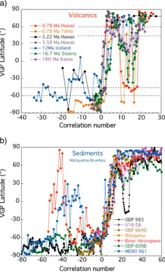
Figure 3. (a) VGP paths for the M-B transition derived from the updated Love and Mazaud [1997] database (see section 3.2) for sedimentary records—some line connec-tions are not meaningful due to a lack of detailed successions of transitional VGPs. Note the smearing of direcconnec-tions and hence of VGP posiconnec-tions caused by U-channel measurements at Site 983. (b) Updated database for volcanic records of the last reversal. The bottom plot contains all VGP positions from the two sites.

Tongjing, China [Zhu et al., 1991], and Chile [Brown et al., 1994]. Any selection of records is subjective because it relies on debatable issues. In the present case, we dispute the choice of Love and Mazaud [1997] in relation to transitional samples that were not stepwise demagnetized (Boso Peninsula and Ocean Drilling Program (ODP) Hole 609B) and sedimentary records with deposition rates of 4 cm/kyr (ODP Holes 609B and 664D), which provide a highly smoothed picture of the transitionalfield. A few other records are also questionable regarding their interpretation. One site from a loess sequence is of doubtful value given the complex remanence acquisition mechanism in loess [Zhao and Roberts, 2010; Wang and Løvlie, 2010; Taylor et al., 2014]. Five sedimentary sites have deposition rates between 4 and 6–8 cm/kyr. All of these VGP trajectories are poorly defined with only two or three VGPs, such as the puzzling record from Boso Peninsula [Niitsuma, 1971] with few intermediate VGP positions, despite a deposition rate 40 times as large as that at the other sites.

Based on these considerations, we retained thefive remaining sedimentary records of Love and Mazaud [1997] to which we added more recent data from the North Atlantic Ocean [Channell et al., 2004]. Each VGP path has been plotted separately in Figure 3a. The dominant characteristic is that they are all different and, thus are consistent with a nondipolar transitionalfield. The second characteristic is that complexity increases with the resolution of the records. This is particularly true for the Japanese and North Atlantic sites that have much faster sediment accumulation rates. In contrast, the VGP trajectories from sites ODP Holes 664D and 609B are poorly defined due to their low deposition rates and, therefore, provide a smeared record-ing of the geomagnetic signal.

We have proceeded the same way to select volcanic records of polarity transitions. We now know that the volcanic record from Chile [Brown et al., 1994], which has been redated [Singer et al., 2005], is not related to the last reversal. Furthermore, the study from Tanjing, China [Zhu et al., 1991], incorporates only three data points from three lavaflows and a sole transitional direction. The same concern exists for the unique inter-mediate VGP position common to a sequence offive flows from Tahiti [Chauvin et al., 1990]. We dispute that this VGP cluster resulted from a short period of volcanic activity and consider it, therefore, as not fully repre-sentative of the reversal process (see sections 4.4 and 4.6). We add two recent volcanic records of the last reversal that were not incorporated in the former database [Love and Mazaud, 1997]. Thefirst [Coe et al., 2004] is from Maui (Hawaii), while the second [Mochizuki et al., 2011] from Tahiti (french Polynesia) completes a former data set [Chauvin et al., 1990] from this location. Figure 3b incorporates about 20 volcanic VGP posi-tions at latitudes<45° with no longitudinal preference and no similar VGP position among the records. We deplore the existence of such a relatively sparse data set. Despite this limitation, these VGP configurations are inconsistent with a dipolar transitionalfield.

3.3. Additional Indications for a Nondipolar Transitional Field

Other studies have reinforced the hypothesis of a nondipolar transitionalfield and that nondipolar field configurations could have dominated during reversals other than the last one. Simple geometrical reversal models, in which nondipolefields are allowed to persist while the axial dipole decays through zero and then builds again in the opposite direction, predict increased reversal duration with latitude, a trend that has also been reported in the numerical simulations [Wicht, 2005; Wicht et al., 2009]. The average trend is not mono-tonic, with duration decreasing from the equator to the tropics and increasing again en route to the pole (e.g., Figure 4.18 in Wicht et al. [2009]). This reflects the fact that the duration of some simulated reversals does not have a clear longitudinal dependence.

Despite our lack of confidence in sedimentary records, we report an observation by Clement [2004] who selected sediment records of the last four reversals and found that the apparent duration of the transitional interval (which represents the thickness of sediment with transitional directions) varies with site latitude. However, this implies that similar processes governed all four reversals and that they had the same duration at each latitude. This is a major assumption which, given the small size of the database, cannot be tested. For this reason, we have restricted our analysis to the last reversal. The picture that emerges from Figure 4a is incomplete with only three Southern Hemisphere sites (that have been plotetd with positive latitudes). Shorter durations are observed in records from low-latitude sites along with longer durations at middle to high latitudes, but the relationship is not without ambiguity due to data scatter. If we take into account the sizes of the error bars, there is roughly a factor of 2 difference in mean duration at sites below 20° latitude and those between 30° and 60°, but there is no clear trend within these two latitudinal groups.

Care should be exercised when dealing with mean deposition rates to calculate durations of short events. Deposition rates can vary rapidly over time intervals as short as a few thousand years. A typi-cal example is provided by a study from Crete [Valet et al., 1988a] with two distinct records of the same reversal from sites located a few kilo-meters away from each other (Figure 4b). The mean deposition rate [Langereis et al., 1984] of section 1 (Potamida) is 1.3 times larger than that at section 2 (Skouloudhiana), but the transitional interval at section 2 is inconsistently twice as thick as that at section 1. The apparent duration of the transition, therefore, differs by almost a fac-tor of 3 between these nearby sections; this cannot be due to the field. The recording differences observed for these neighboring sections with the same environmental conditions could also occur for sections separated by thousands of kilometers and limits analysis of transitional records. Another factor to consider is the complexity of the process associated with precursory and/or rebound phases within a transition with significant duration (see section 6.1). At low deposition rates these phases can be mixed in the record or at least generate large biases. In the study of Clement [2004] low-and high-latitude records are both characterized by different deposition rates; therefore, the rela-tionship found by the author must imply the absence of correlation between the thickness of transition zones and deposition rates if it isfield dependent. This has been tested and gives further credit to the results. It is impossible to establish the chronology for transitional superimposed lava flows and, therefore, such records are not compatible with the approach of Clement [2004]. Notwithstanding that, if we refer to the short period during which the VGP transits between the two geographic poles, the few high-latitude records contain more intermediate directions than low-latitude ones. Keeping these restrictions in mind, we are tempted to favor a latitudinal dependency of reversal duration, but a larger number of records, particularly with deposition rates between 6 and 12 cm/kyr, remains crucial to validate the relationshipfirmly.

3.4. Modeling the Harmonic Content of the Transitional Field

A primary goal when studying reversals is to determine the harmonic content of the transitionalfield. Four attempts have been made so far. It is not surprising that all studies have focused on the last reversal. In addition to the need for good quality directional and paleointensity variations, a major difficulty is to estab-lish the simultaneity offield changes recorded from remote places in order to align all events on a common time scale. The task is even more difficult because nondipolar field components are supposed to generate differentfield changes depending on location.

Mazaud [1995] sought the best correlation between VGP latitudes recorded at different sites. He assumed that VGPs cross the equator simultaneously at all sites. However, given that a nondipolefield likely governs transitions, this assumption will not be valid [Quidelleur and Valet, 1996; Brown et al., 2007; Valet and Plenier, 2008], even with a static nondipolarfield.

a)

b)

Figure 4. (a) Duration of the last reversal derived from sedi-mentary records [Clement, 2004] as a function of site latitude. (b) Thickness of transitional intervals (black intervals) that corresponds to the same Miocene reversal recorded in adjacent sedimentary sequences from Crete.

Shao et al. [1999] followed another approach using a scheme based on Maxwell’s multipole theory. They used the database compiled by Athanassopoulos et al. [1995] for the last reversal, which was an exhaustive compi-lation of all reversal studies without any selection and is therefore governed by a majority of meaningless low-resolution sedimentary records.

Leonhardt and Fabian [2007] used an original approach based on an iterative Bayesian scheme to construct a global model of the MB transitionalfield up to spherical harmonic degree 4. The model describes the field evolution derived from four studies (ODP holes 664D, 609B, core V16-58 for sediments, and the ME-ET sec-tions for volcanics). In a second step, thefield changes predicted at several other locations are tested against existing records at the same locations. This approach appears suitable; however, we again question the choice of the database. The records from sites ODP Hole 664 and core V16-58 have low resolution with deposition rates from 4 to 2.5 cm/kyr and few transitional data points, while the volcanic sections ME-ET at La Palma do not incorporate any transitional directions and therefore bring no constraint to the problem.

The model of Leonhardt and Fabian [2007] has been tested by comparing its predictions against eight other independent records from different geographical locations. Even complex VGP movements are remarkably well predicted for most independent sites, but these optimistic conclusions cannot be validated. The record from ODP site 792 (Northwest Pacific Ocean) includes only two transitional VGPs and is, therefore, not testa-ble. The record from site RC15-21 has a deposition rate as low as 1.1 cm/kyr, which is not suitable for a reversal study. Note also that the data from ODP Hole 883B [Athanassopoulos et al., 1993] have never been published and are in full disagreement with the model prediction. Moreover, the authors incorporated results from the LL section at La Palma [Quidelleur and Valet, 1996] that are not related to the last reversal, and from Lake Tecopa which, despite fair agreement with the model, has been shown to be remagnetized [Larson and Patterson, 1993]. The fact that the model predictions can be defended from inadequate data is puzzling. Not only does it emphasize the need to select appropriate data with regard to objectives but it also points out a great deal of subjectivity when comparing model predictions.

The most recent global model of the last transition goes up to degree 3. It was attempted by Ingham and Turner [2008] from 11 records but only from 10 distinct sites, considering that two records (ODP sites 983 and 984) are from nearby localities in the North Atlantic Ocean [Channell and Kleiven, 2000; Channell et al., 2004]. Five records were included while two others were rejected from the compilation by Love and Mazaud [1997] based on lack of resolution. The three remaining records are from more recent studies, but they are hampered by problems that limit their usefulness. Thefirst record was obtained from California margin sediments and was described by the authors [Heider et al., 2000] as being affected by a strong coring-induced overprint that gave rise to false transi-tional directions. In addition, VGPs for the normal and reverse polarity directions that surround the reversal do not reach the geographic North and South Poles. The second record from rapidly deposited sediments cored in the Celebes and Sulu Seas [Oda et al., 2000] incorporates only two intermediate directions with equatorial VGPs and no data between the North Pole and South Pole positions due to the scarce sampling. Lastly, a record from ODP Hole 1082C in the South Atlantic Ocean [Yamazaki and Oda, 2001] was obtained from two data sets that yield different transitional results: the studied U-channel samples have many transitional directions, while the discrete samples define two successive phases with a precursor and a transition with few transitional data. The U-channels have smeared the signal and generated transitional directions that cannot be validated by the single-sample data. During the reversal, the dipole and axisymmetrical quadrupole change polarity while the other Gauss coefficients retain values close to those of the present field with some random noise. The Gauss coefficients that describe the model were then used to generate reversal data at the 10 sites that correspond to locations of studied reversal records, all from sediments.

In contrast to Leonhardt and Fabian [2007], Ingham and Turner [2008] compared a few predictedfield changes with those derived from the corresponding paleomagnetic record. How far can we compare the predictions of these two models? They bothfind that through the reversal the dipole and nondipole fields had approxi-mately equal intensities, which may result from the time averaging inherent to sedimentary records. The non-dipolefield appears to be weakened at some point in the former model, while this is not the case for the later model. The model of Ingham and Turner [2008] contains a large excursion prior to the transition that does not appear in the Leonhardt and Fabian [2007] model due to their choice of sites. It is puzzling that no dipole decrease accompanies the prereversal excursion. Except for a short period, the nondipole/dipole ratio is strikingly different between the two models.

4. Features of the Transitional Field

No complete documentation of transitionalfield behavior has yet been provided by paleomagnetic records. Therefore, results are often split between arguments that support a direct geophysical interpretation and those that question the suitability of the measured paleomagnetic signal. One can defend a consensus that emerges when a specific feature is documented repeatedly by records of various origins. Nevertheless, this is not straightforward because artificial features can be induced by the magnetization process and/or by inac-curacies in determining the timing of events. Controversies about the existence of preferred longitudinal VGP bands or the origin of directional clusters are typical cases that demonstrate this point.

4.1. Preferred VGP Locations

Among the earlier models proposed for reversals, Bogue and Coe [1984] suggested a standingfield that persisted during successive reversals and, therefore, produced recurrent VGP trajectories when observed at the same site (the standing component being nondipolar). This concept of recurrent mechanisms over long periods of time was given a geophysical meaning after being further promoted in a different way as described below.

Although sediments fail to record rapid nondipolarfield components, we cannot discard the concept that they retain a memory of persistent long-term geomagnetic features. Clement [1991] observed that sedimen-tary records of the last reversal are constrained within two“preferred longitudinal bands” almost 180° apart from each other. In the meantime Tric et al. [1991] and Laj et al. [1991, 1992] reached similar conclusions from a larger set of records distributed between the late Miocene and the last reversal. They noticed that the two longitudinal VGP bands correlated with regions of high seismic velocity in the lower mantle [Dziewonski and Woodhouse, 1987] and, thus, with cold and/or dense material at the base of the mantle. They also lie close to regions of magneticflux concentrations in the historical field [Bloxham and Jackson, 1992; Jackson et al., 2000]. For thefirst time, the concept of mantle control on the reversing field could be directly associated with paleomagnetic observations [Gubbins, 1994].

4.2. What Mechanism?

Before discussing the aspects related to the database of polarity transition records, the question that comes to mind is by which mechanism structural seismic anomalies constrain pole locations during reversals. Dynamical coupling between core and mantle would establish steady conditions at the core-mantle bound-ary (CMB) that would persist long enough to give rise to recurrent transitionalfield features. Runcorn [1992] proposed that electromagnetic torques originating from a heterogeneous electrical conductivity distribution in the lowermost mantle would tend to bias the weak transitionalfield toward mantle structures. This sce-nario was further studied by Brito et al. [1999] using an analytical model that included resistive torques in addition to the driving torques previously considered by Runcorn [1992]. This led Brito et al. [1999] to draw the opposite conclusion, namely, that lateral variation in lower mantle conductance was unlikely to affect the VGP path during a reversal. To our knowledge, this issue has not since been addressed using numerical simulations and may be worth reconsidering when further constraints are placed on the conductivity distribution in the lowermost mantle, particularly in connection with postperovskite phase transition [Ohta et al., 2008].

Alternatively, and because mantle and core are heat engines operating on vastly different time scales, the heatflux imposed by the mantle on the underlying core at the CMB can be considered as being static when studying core dynamics on magnetic diffusion time scales (tens of thousands of years). Lateral variations of the heat flux imposed by temperature inhomogeneities in the lower mantle influence core flow. Glatzmaier et al. [1999] imposed a nonuniform heatflux pattern on a reversing dynamo model and found a crude correlation between the density of transitional VGPs and the pattern of heat flux at the CMB (their Figure 1d), an analysis based on a limited number of simulated reversals (see also the discussion in Glatzmaier and Coe [2015]). More recently, Kutzner and Christensen [2004] used a three-dimensional convection-driven numerical dynamo with imposed nonuniform CMB heatflow and found, based on a much larger number of reversals, that the VGPs have a tendency to fall around longitudes of high heatflow. They pointed out the role of the equatorial dipole in favoring longitudinal VGP bands. Stronger heatflow induces flow convergence and hence stronger magnetic flux, and therefore a preferred location (on average) for the equatorial dipole. As physically sound and satisfactory as this mechanism can appear, a caveat is that the heat

flux heterogeneity must be large in the simulations, representing a significant portion of the heat con-ducted along the adiabat, for this geographical localization to be effective. Interestingly, VGPs in the pre-sent NADfield are found along the western Pacific rim [Valet and Plenier, 2008], but this large preference disappears after removing the equatorial dipole contribution. Given its permanent and rapid evolution (as directly observed from the archeomagnetic database) we can wonder by which process the equatorial dipole generates a long-term recurrent pattern, unless it is assumed that despite its permanent motion, the present orientation has been dominant over the past million years. The mechanism proposed by Kutzner and Christensen [2004] enables such long-term mantle control, but again, it is not certain because it requires large heatflux contrasts. These contrasts (expressed as a fraction of the heat conducted along the adiabat) become even more questionable as the recent increase in estimated core thermal conductiv-ity has precisely multiplied by a factor of 2 to 3 the heat conducted along the core adiabat (see Hirose et al. [2013] for a review).

4.3. A Few Possible Artifacts

Most sites represented in the database are far from being uniformly distributed around the globe, but they, too, are concentrated within two antipodal longitudinal bands approximately 90° away from the pre-ferred transitional VGP longitudes [Valet et al., 1992; McFadden et al., 1993]. Moreover, this initial compilation included a few controversial records such as a dominant VGP trajectory (in terms of the number of intermedi-ate directions) that was recorded by the authigenic mineral greigite [Tric et al., 1991] and is, therefore, not appropriate for transition studies [Roberts et al., 2005, 2011]. Several scenarios, including nonantipodal stable directions before and after a reversal [Langereis et al., 1992], as well as the influence of inclination shallowing [Barton and McFadden, 1996] or the enhanced role of gravity and hydrodynamic forces on settling magnetic particles (see section 3.1), have been raised to account for the two antipodal longitudinal bands. The debate is still alive, but a few other observations cast additional doubt about the geomagnetic origin of VGP paths found within preferred longitudinal bands.

It is striking that the most detailed records from the North Atlantic Ocean [Channell et al., 2004] with deposi-tion rate larger than 10 cm/kyr and those from Japan [Okada and Niitsuma, 1989] with deposideposi-tion rate larger than 300 cm/kyr do not have longitudinally confined VGPs but successions of latitudinal and longitudinal crossings. The North Atlantic records also contain VGP clusters, but they could have been generated partially by signal smearing by the response curve of the magnetometer [e.g., Nagy and Valet, 1993; Weeks et al., 1993] during continuous measurements of long sediment sections. This effect can be illustrated by comparing the directions measured by this technique with those obtained from a suite of single samples adjacent to each other from the same sequence. Directional changes associated with the last reversal measured at the same depths in U-channels and single samples from core MD90-961 have marked discrepancies (Figures 5, top and 5, bottom). The VGPs derived from the U-channels are more concentrated than those of the single sam-ples and contain clusters that are not so strongly present in the single-sample data. This is a consequence of measurement smearing. Evidently, the characteristics of the record can vary because the volume of sediment integrated by continuous measurements is much larger than for single samples. Some results from ODP Site 983 demonstrate that U-channel measurements havefiltered large-amplitude changes revealed by single samples, so that at some stratigraphic levels the results differ by up to 40° in inclination (see Figures 10–12 in Channell et al. [2004]).

The overall similar configuration of VGP paths of three distinct North Atlantic records pleads in favor of their geomagnetic origin. However, the detailed directional changes differ between the three records. The com-plexity of the North Atlantic VGP trajectories contrasts sharply with the smooth aspect of VGP paths obtained for records from sediments with lower deposition rates. The resolution of the records from rapidly deposited sediments is high enough to resolve rapid time-varying nondipole components during the transition, while the lower resolution records have been time-averaged.

4.4. Long-Lived Transitional Field States: The Geomagnetic Scenario?

There is little evidence for continuous VGP movement in volcanic reversal records. Concentrating on a selec-tion of six data sets fromfive sites over the past 10 Ma, Hoffman [1991, 1992] reported the existence of two transitional VGPs clusters; one centered over western Australia and the other one off the southeast coast of western America. They were both interpreted as reflecting specific inclined dipolar field configurations. In a

subsequent paper concerning the last reversal, Hoffman [2000] described the dominance of two pairs of low- and middle-latitude VGP concentrations that are mirrored about the equator and concluded that the M-B reversal was dominated by quasi-stationary low harmonic order states. It was pro-posed that a transitional state was reached early after the transition onset, held for a considerable time, and that the reversal was rapidly completed much later. The VGP clusters are possibly connected to the apparent preferred longitudinal VGP bands observed in sediments, because smoothing inherent to magnetization acquisition generates longitudinally confined transitional VGPs by the smearing of clusters that lie within or close to the preferred longitudinal bands.

Two issues lie behind the concept of long-lived transitionalfield states that we discuss separately. The first con-cerns the origin of clusters within a sin-gle reversal, while the second is related to the recurrence of the same clusters during different reversals.

The presence of a patch of recurring VGPs during a reversal suggests that the geomagnetic field retained the same inclined dipolar configuration for a certain period of time provided that the patch is observed globally. This interpretation relies on the assump-tion that each individual lavaflow provides a unique and independent record of the local field. However, successiveflows with the same direction can also be generated by closely spaced eruptions. In this case, VGP clusters would represent a unique, almost instantaneous, picture of thefield. The “volcanic” hypothesis assumes that directional clusters result from rapid successive eruptions, whereas in the “geomagnetic” scenario thefield remained stable for a long period of time. It is impossible to test the two hypotheses using radiometric dating. If we refer to the historicalfield, the rate of geomagnetic changes varies with time and location. The recent geomagnetic declination has changed in Europe by 10° in about 80 years, which can be considered as a lower limit of resolution for paleomagnetic records. Thus, redundant directions can be recorded over a few hundred years, which is compatible with the frequencies of volcanic eruptions.

4.5. Long-Lived Transitional Field States: The Volcanic Scenario?

No unambiguous test exists to discern whether VGP clusters reflect intense volcanic activity or standstills in the geomagnetic reversal process. In principle, the same weight must be given to both hypotheses. However, volcanic activity is characterized by periods of quiescence followed by periods of intense activity and reports of historical eruptions suggest that the volcanic explanation makes sense. The existence of VGP clus-ters has also been reported in a few sedimentary records but their interpretation can be subjective. A typical example is the record of the Gauss-Matuyama reversal from the sediments of Searles Lake (California) [Glen et al., 1994, 1999], if we exclude the possibility that potential coring disturbances generated large directional changes interpreted as excursions like in another core drilled at Owens Lake using the same technology [Rosenbaum et al., 2000]. The VGP path has been described as a succession of clusters, but it can as well be

Figure 5. Comparison of VGP paths derived from measurements of (top) single samples with those obtained from (bottom) U-channels at the same spatial resolution. Note the emergence of VGP clusters (yellow areas) generated by smearing introduced by the response function of the mag-netometer for U-channel measurements.

interpreted as a continuous and regular VGP evolution punctuated by short variations in deposition rate. Surprisingly also for the CMB control hypothesis, one of the clusters lies above North Africa which is above a zone of slow lower mantle shear wave velocities, while, according to the data and models mentioned above, VGPs are expected to fall above zones of high heatflow and, therefore, fast shear wave velocities. If clusters represent long-lived transitionalfield states, they must have lasted long enough to have a chance of being documented in most, if not all, sequences that recorded the same reversal. A few reversals recorded in parallel sequences of superposed volcanicflows that are only a few kilometers away from each other pro-vide interesting indications as discussed below. Thefirst study of Van Zijl et al. [1962] of a reversal recorded by the Stronberg lavaflows in South Africa has been reinvestigated at another locality by Prévot et al. [2003] and more recently by Moulin et al. [2012]. Three parallel sections reveal the same dynamical structure, and parti-cularly the existence of a large elongated loop with VGPs that cluster to the southeast of Asia. However, none of the three records have the same number of stationary poles, whereas VGP clusters at the same location in the three sections should reflect a long stationary field state if the same flows are present. The other example involves the Steens Mountain reversal data set, which is the most detailed volcanic record of a reversal. It con-tains a series of VGP clusters recorded from sections 60 km apart by lavaflows with different chemistry. In addition, one VGP cluster (located in western South America) is visited twice early and late in the record, which reinforces the concept of a correlation with the fast seismic velocity zone beneath this area, although it is puzzling that the same record also contains a cluster over North Africa again above a zone of lower man-tle low shear wave anomalies.

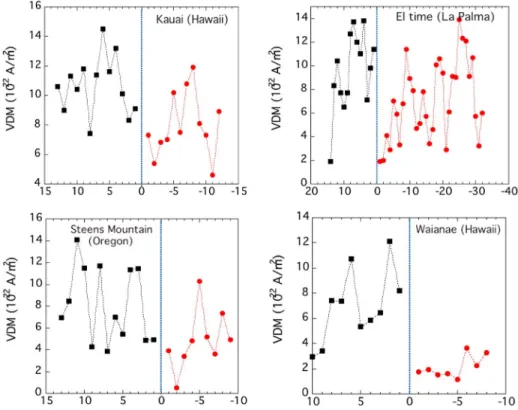
Two other studies of parallel volcanic sequences have been connected to each other to provide additional information. An intriguing observation in favor of episodic volcanism comes from the record of the Upper Mammoth transition [Herrero-Bervera and Valet, 1999, 2005] from several nearby sequences in Waianae volcano (Hawaii). Each sequence records different VGP distributions, which sometimes cluster at the same location with a different number of lavas and sometimes not, while they are separated by a few kilometers at most. Similarly, a link between transitional directions and volcanic activity can be derived from parallel Icelandic sections that recorded the R3-N3 reversal which likely corresponds to the Matuyama-Réunion rever-sal. The sections were initially studied by Sigurgeirsson [1957] and Wilson et al. [1972], and they have been subsequently revisited by Goguitchaichvili et al. [1999]. The evolution of VGP latitude plotted in Figure 6 reveals that each section records the same geomagnetic features but that the VGP cluster found close to the equator is different in each sequence. Of particular interest is the relationship between the resolution of the cluster and the geographical location of each sequence. The most detailed cluster was obtained at sec-tion PV likely close to the eruptive center and the number of clustered VGPs decreases with distance away from section PV. At the farthest location away from PV, section KY has a relatively regular VGP distribution while section SB did not record any intermediate VGP. Distance from the eruptive center was the unique factor that controlled the number of lavaflows produced during this period. If we assume that these succes-sive lavaflows covered a long period during a stationary field state, there is no reason why it would not be recorded at least once. We infer that these records with clustered VGPs were generated by rapid eruption fre-quency and that they were controlled by the size of the event which likely reflects gradual depletion of the magma chamber.

Another point to consider in relation to transitional VGP clusters is the apparent recurrence of a few spots (like Australia) mentioned in some studies that are discussed below. Evidence for recurrence of the same VGP clus-ter recorded from distant sites during the same reversal would provide evidence for a geophysical origin of each cluster.

4.6. Are VGP Clusters Related to Field Anomalies?

Hoffman and Singer [2008] related the most intense geographicalflux lobe of the present NAD field over Australia to the location of the VGP cluster derived from a selection of transitional data at Tahiti to argue for long-termfield anomalies that are important for transitional fields. If we refer to the NAD during the past thousand years and not only the past 100 years as considered by Hoffman and Singer [2008], there is no evi-dence for persisting stationary features. Flux lobes exist, but they appear and disappear. This might, however, reflect the type of prior information used to build time-dependent geomagnetic field models over the past few millennia (see Korte and Holme [2010] for details). Hoffman and Singer [2008] noticed that in contrast the VGPs of an excursion recorded from the Eiffel volcanics are spread over Eurasia, because this locality is

located far from the influence of prominent concentrations of NAD field flux. In both cases, the authors argued that the NADfield dominated the transition and resulted from motions generated in Earth’s upper core. Thefield pattern is argued to have been controlled strongly by physical variability of the lower mantle. This suggestion implies that a given cluster should be observed during successive events at the same geographical locality, but not from everywhere.

Support for these concepts relies on a subset of paleomagnetic records but ignores the rest of the database. We selected the detailed volcanic records from sequences of superposed lavaflows including at least five dis-tinct transitional VGP positions and several reversed and normal polarityflows surrounding the reversal. Only 10 records satisfy these criteria that guarantee that we are dealing with actual reversal records without uncer-tainty about the chronological succession of events. The individual VGP paths are shown in Figures 7a–7k. The number of intermediate VGPs remain poor to drawfirm conclusions. In the present state of the database, we can simply mention that there is no systematic reproduction of VGP clusters over Australia and America and that clusters are also present at other locations like central Europe, mid-North Africa, and the mid-South Pacific which are neither linked to preferential longitudinal bands, nor to long-term field anomalies. More

Figure 6. (a) Evolution of VGP latitude recorded infive parallel sequences of overlying lava flows. In each case a group of VGPs is present at the same low-latitude position, but the number of VGPs differs between each sequence. (b) The decreasing number of VGP positions depends on the distance of theflow from the eruptive center, which is close to location PV. Redrawn from Goguitchaichvili et al. [1999].

specifically, the two detailed volcanic studies of the last reversal shown in Figures 7a and 7b, which were not included in the Hoffman and Singer [2008] analysis, do not indicate the existence of VGP clusters.

Four records contain VGPs in the vicinity of Australia. The most significant groupings are present for the Réunion event (2.2 Ma) recorded in Iceland (Figure 7h) and in the 61 Ma reversal from Greenland (Figure 7k). The other two clusters concern the M-B transition with one VGP over Australia and the Upper Jaramillo (0.99 Ma) from

Figure 7. (a–k) VGP paths of the most detailed volcanic records of reversals. Red (blue) VGP paths correspond to reverse-normal (normal-reverse) transitions. Data are from: Coe et al. [2004], Chauvin et al. [1990], Mochizuki et al. [2011], Herrero-Bervera and Valet [1999], Herrero-Bervera et al. [1999], Moulin et al. [2012], and Riisager et al. [2003].

Tahiti with two VGPs over Australia, which, therefore, cannot be considered clusters. We could add the Big Lost event pointed out by Hoffman and Singer [2008] (but this record does not satisfy our selection criteria) that contains “Australasian” VGPs according to the name given to this patch. Altogether these results are at first glance neither consistent, nor fully inconsistent with the suggestion of Hoffman and Singer [2008]. However, we should expect VGP clusters in the records from Hawaii, but they are not present. In contrast, no Australasian cluster should be observed in the high-latitude records, yet such directions occur in the too high latitude records.

The hypothesis of preferred VGP paths has been tested several times using volcanic records. The conclusions of Prévot and Camps [1993] defending the proposed uniform distribution of transitional volcanic VGPs were dis-missed by Love [1998]. Although the two databases used for the respective analyses were more or less the same, the data treatments were different, which again raises questions about field sampling by lava flows. Prévot and Camps [1993] considered similar directions to mostly coincide in time and, thus, must be combined into a single direction, while Love [1998] defended the opposite. A second dif-ference was that Love [1998] weighted the data to account for the fact that transitions are recorded by widely differing numbers of intermediate directions. This approach was initially followed for sediments [Valet et al., 1992] to compensate for differences (sometimes up to a factor of 30) in resolution between individual records and also becausefield changes are heavily smoothed by the magnetization acquisition process. Most trajec-tories are longitudinally constrained, so that the weighting procedure does not introduce any change in the final information with respect to a nonweighted detailed trajectory. However, the VGP paths of the most detailed volcanic records are complex and therefore contain significant geomagnetic information that is truncated and, thus, lost after weighting. The weighting procedure is, therefore, questionable for volcanic records, especially when VGPs are scattered over the globe. Lastly, it is worth mentioning that most VGPs in the compilation have high latitudes (say between 50° and 60°) and are not representative of a transi-tional state.

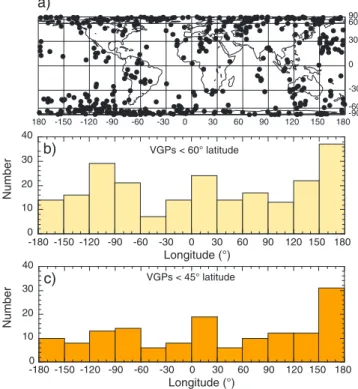
In Figure 8 we plot all intermediate volcanic VGPs (Figure 8a) (from the previous selection of records) with a frequency histogram within 30° longitudinal bands after selecting VGP latitudes<60° (Figure 8b) and >45° (Figure 8c). The VGP positions are widely scattered and lie within all longitudinal bands. Higher fre-quency is found within the 60° to 120°W sector over the American continent, which is caused by a group of VGPs at northern intermediate latitudes in the Steens Mountain record [Jarboe et al., 2011]. A second band exists between 120°E and 180°E, but largely disappears after restraining the selection to VGPs below 45° lati-tude; the group of VGPs at midnorthern latitudes within the 150°–180°E sector (Figures 7f and 8a) belong to the Steens Mountain record and, therefore, bias the results (Figure 8c) toward a single record, which is not representative of a geomagnetic cluster. Note that there is also some preference of VGPs for the African long-itudinal band in both selections. In summary, the existence of preferred longitudes depends on data selection and, therefore, has no stable solution yet. Such instability points to the difficulty in performing a meaningful statistical treatment of the VGP distribution within each longitudinal band. In addition, recurrent VGPs from different records within the same longitudinal band do not mean that they belong to the same time period

-150 -120 -90 -60 -30 0 30 60 90 120 150 180-90 -60 -30 0 30 60 90 0 10 20 30 40 -180 -150 -120 -90 -60 -30 0 30 60 90 120 150 180 Longitude (°) 180 Number 0 10 20 30 40 Longitude (°) Number -180 -150 -120 -90 -60 -30 0 30 60 90 120 150 180 a) b) c)

Figure 8. (a) VGP positions of the volcanic reversal records shown in Figure 7. (b) Histogram of the frequency of VGPs in terms of longitude. (c) Same as Figure 8b but for VGPs with latitude lower than 45°.