CubeSat constellation implementation and management using differential drag

CubeSat Constellation Implementation and

Management Using Differential Drag

by

OF TECHNOLOGY

Zachary Thomas Lee

_IJUL

112017

B.S. Mechanical Engineering

United States Military Academy, 2015

LIBRARIES

Submitted to the Department of Aeronautics and Astronautics

ARCHIVES

in partial fulfillment of the requirements for the degree of

Master of Science in Aeronautics and Astronautics

at the

MASSACHUSETTS INSTITUTE OF TECHNOLOGY

June 2017

Massachusetts Institute of Technology 2017. All rights reserved.

Signature redacted

A uthor ...

Department

ronaucstronautics

,

eoatic and Atoatc

May 25, 2017

Certified by...Signature

redacted

V

_{Kerri Cahoy}

Associate Professor of Aeronautics and Astronautics

Thesis Supervisor

Accepted by...Signature

redacted

Youssef M. Marzouk

Disclaimer: The views expressed in this thesis are those of the author and do not reflect the official policy or position of the United States Army, the United States

CubeSat Constellation Implementation and Management

Using Differential Drag

by

Zachary Thomas Lee

Submitted to the Department of Aeronautics and Astronautics on May 25, 2017, in partial fulfillment of the

requirements for the degree of

Master of Science in Aeronautics and Astronautics

Abstract

Space missions often require the use of several satellites working in coordination with each other. Industry examples include Planet, which is working to develop a constellation of over 100 Cube Satellites (CubeSats) to obtain global imagery data daily, and Astro Digital, which seeks to implement a constellation of multispectral imaging satellites to image the entire Earth every three to four days [1, 2]. CubeSat constellations are also being considered for applications such as secure laser commu-nication relays and for weather sensing with short revisit times [3, 4]. Such missions require several CubeSats with regular spacing within an orbital plane to achieve their objectives.

However, an appropriately arranged constellation can be particularly difficult to implement for CubeSats. Cold gas propulsion systems with the ability to provide tens of meters per second of delta-V (for a 3U CubeSat) exist and can be used for constel-lation management on timescales of weeks [5, 6, 7, 8, 9]. Monopropellant systems also currently exist for CubeSats, but, like cold gas systems, they can require significant power, mass, volume, and thermal management resources, and they also carry more risk [9, 10]. Launch services providers often limit acceptance of pressurized vessels, which can limit launch opportunities for CubeSats with cold gas or monopropellant propulsion systems. Although electric propulsion systems can provide up to 100 m/s delta-V for a 3U CubeSat, they also have mass, volume, cost, and power impacts, and they typically require timescales on the order of weeks to months to cause significant changes [6, 11, 9].

In low Earth orbit, there is sufficient drag to perturb satellite orbits. Though it varies widely based on conditions, at 500 kilometer (km) altitude, the acceleration due to drag on a 3U CubeSat can be around 15 ' per unit area [12]. Over time, this is enough acceleration to change a satellite's orbit. By controlling the attitude

100 days.

Previous work with differential drag for constellation management has focused on linearized control schemes for formation flight. However, the linearized equations used for close-proximity flight are not valid for maximum-separation missions [13, 14,

15]. While some work does exist on maximum-separation missions, conditions are

simplified or details on the estimation and control scheme are omitted or inadequate

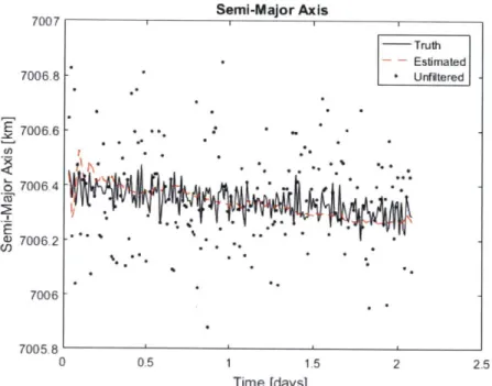
[8, 16, 17, 18, 19]. This work uses an unscented Kalman filter to estimate mean orbital

elements and a novel control scheme to first offset and then match relative mean semi-major axes. The separation of mean semi-semi-major axes creates different mean motions such that allow for the relative mean anomalies to be controlled. Simulation results demonstrate that differential drag can be used to control and maintain satellites within 0.5 degrees of the desired mean anomaly relative to other satellites. For two satellites in the same orbital plane at 500 km altitude seeking to maximize separation,

0.5 degrees corresponds to an angle that can be traversed in under 10 seconds. For

Earth observation mission, this has a negligible effect on revisit times and can be considered an acceptable result.

Thesis Supervisor: Kerri Cahoy

Acknowledgments

While not without its difficulties, earning my degree at MIT has been an incredible journey, and I am so thankful to have had the opportunity to study and conduct research at MIT and Lincoln Laboratory. Having the support of my friends, family, and peers has meant more to me than words can express.

Specifically, I would like to thank Professor Kerri Cahoy, my thesis advisor, for her guidance throughout my time at MIT. From the day I started to now, I have grown so much, and I could not have achieved this without Kerri. I would also like to thank Michael DiLiberto, Bill Blackwell, Dan Cousins, and Weston Marlow for mentoring me and taking the time to welcome me into a new project and teach me throughout my time working at Lincoln Laboratory. The entire MiRaTA team has taught me about satellite engineering, and they have made my experience a rewarding one. I am grateful to have worked with such an amazing team.

My parents and brothers have always been supportive in my endeavors. Studying

at MIT has been a dream of mine since I was a teenager, and I would not be here without the support of my family. Lastly, my friends have consistently encouraged me to pursue my goals, and this has helped keep me motivated throughout graduate school. Simply put, I could not have graduated MIT without the support of those close to me.

Contents

2.2.3 Gauss's Variational Equations . . 2.2.4 Mean Orbital Elements . . . .

2.2.5 Clohessy-Wiltshire Equations . . 2.3 Propulsion . . . . 2.4 Global Positioning System . . . .

2.5 Two-Line Elements . . . .

2.6 Orbit Estimation . . . .

2.6.1 Unscented Kalman Filter . . . . .

2.7 Attitude Determination and Control

2.7.1 Sensors . . . .

2.7.2 Actuators . . . .

2.7.3 CubeSat Performance . . . .

2.8 Orbit Control through Differential Drag

3 Modeling and Simulation Approach 3.1 Chapter Overview . . . . 3.2 Simulation Overview . . . . 3 5 7 9 10 11 13 13 13 18 20 21 22 22 22 23 24 34 36 38 39 41 42 42 46 49

50

3.2.1 Orbit Propagation . . . . 58

3.2.2 Simulation Parameters . . . . 60

3.3 E stim ation . . . . 61

3.4 C ontrol . . . . 64

3.5 Case Studies . . . . 69

3.5.1 Case Study 1: NPSCuL 8-CubeSat Deployer . . . . 71

3.5.2 Case Study 2: TROPICS Low Inclination Orbit . . . . 73

3.5.3 Case Study 3: Polar, Elliptical Orbit . . . . 74

3.5.4 Case Study 4: Planet Flock 1-C Comparison . . . . 75

3.5.5 Sensitivity Study on Implementation Time . . . . 76

3.5.6 Station Keeping After Implementation . . . . 77

3.6 Additional Considerations . . . . 77

3.6.1 Reaction Wheel Saturation . . . . 78

3.6.2 Orbit Lifetime . . . . 78

3.6.3 Power Generation . . . . 79

3.7 Chapter Summary . . . . 79

4 Analysis and Results 80 4.1 Chapter Overview . . . . 80

4.2 UKF Performance for a Single CubeSat in Case 3: Polar, Elliptical Orbit 80 4.3 Results for Case Study 1: NPSCuL 8-CubeSat Deployer . . . . 85

4.4 Results for Case Study 2: TROPICS Low Inclination Orbit . . . . 90

4.5 Results for Case Study 3: Polar, Elliptical Orbit . . . . 92

4.6 Results for Case Study 4: Planet Flock 1-C Comparison . . . . 95

4.7 Sensitivity Study on Implementation Time . . . . 98

4.8 Station Keeping After Implementation . . . . 99

4.9 Chapter Summary . . . . 102

5 Conclusion and Future Work 104 5.1 Sum m ary . . . . 104

5.2 Research Contributions . . . . 105

5.3 Future W ork . . . . 105

List of Figures

1-1 _{Number of CubeSat launches by year from 2005 to 2015 [30] 15}

1-2 _{CubeSat mission status [42] . . . . 17}

1-3 _{TROPICS constellation concept [3]. . . . . 19}

1-4 _{Satellite size comparison . . . . 20}

2-1 _{A highly exaggerated depiction of Earth's oblateness [51] . . 25}

2-2 _{Types of spherical harmonics [52] . . . . 25}

2-3 _{Nodal regression due to Earth's oblateness [57] . . . . 27}

2-4 Apsidal precession due to Earth's oblateness [57] . . . . 27

2-5 US 1976 Standard Atmosphere Density Profile [61] . . . . 30

2-6 The International Space Station altitude during the Halloween storm s of 2003 [63] . . . . 31

2-7 _{Orbit lifetimes for LEO satellites with different drag profiles 32} 2-8 _{The Surrey Training, Research, and Nanosatellite} Demon-strator: A 3U CubeSat with single-deployable solar panels [6 4 ] _{. . . . 3 2} 2-9 _{Effect of disturbing forces by altitude [12] . . . . 34}

2-10 Osculating and mean semi-major axis for a LEO satellite . . 37

2-11 LVLH frame of reference (y is in the direction of the velocity vector) [69] _{. . . . 39}

2-12 Truth, estimated, and unfiltered semi-major axis . . . . 44

2-13 An ADCS block diagram [90] . . . . 51

2-14 CubeSat altitudes [26] . . . . 53

2-15 Simple satellite separation using differential drag . . . . 55

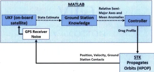
3-1 _{High-level block diagram of simulation . . . . 58}

3-2 _{Satellite drag profile comparison . . . . 59}

3-3 _{Planet's satellites' relative mean anomalies (blue lines} repre-sent high-drag windows) [18] . . . . 66

3-4 The MiRaTA CubeSat [99] . . . . 70

3-5 The N PSCuL [34] . . . . 72

4-1 _{Estimation of the mean semi-major axis (Case 3: Polar,} El-liptical O rbit) . . . . 81

4-2 Estimation of the mean eccentricity (Case 3: Polar, Elliptical O rb it) . . . ... . . . . 82

4-3 Estimation of the mean inclination (Case 3: Polar, Elliptical Orbit) ... ... 82

4-4 Estimation of the mean right ascension of the ascending node (Case 3: Polar, Elliptical Orbit) . . . . 83 4-5 Estimation of the mean argument of perigee (Case 3: Polar,

Elliptical O rbit) . . . . 83 4-6 Estimation of the mean anomaly (Case 3: Polar, Elliptical

Orbit) ... ... 84

4-7 Case 1: NPSCuL 8-CubeSat Deployer orbit clusterness (with-out control) . . . . . 85

4-8 Case 1: NPSCuL 8-CubeSat Deployer orbit clusterness (with control) ... ... 86

4-9 Case 1: NPSCuL 8-CubeSat Deployer relative semi-major axes (with control) . . . . 87

4-10 Case 1: NPSCuL 8-CubeSat Deployer relative mean

anoma-lies (w ith control) . . . . 88

4-11 Case 2: TROPICS Low Inclination orbit clusterness ... 90

4-12 Case 2: TROPICS Low Inclination orbit relative semi-major

axes ... ... 91

4-13 Case 2: TROPICS Low Inclination orbit relative mean anoma-lies ... ... 92

4-14 Case 3: Polar, Elliptical orbit clusterness ... 93

4-15 Case 3: Polar, Elliptical orbit relative semi-major axes . . .. 94

4-16 Case 3: Polar, Elliptical orbit relative mean anomalies . . . . 95

4-17 Case 4: Planet Comparison clusterness . . . . 96

4-18 On-orbit relative arguments of latitude (Case 4: Planet

Com-parison) [18] . . . . 97

4-19 Case 4: Planet Comparison simulation relative arguments of

latitu d e . . . . 97

4-20 Station Keeping clusterness for Case 2: TROPICS Low

Incli-nation (no control from day 173 to day 273) . . . . 100

4-21 Station Keeping relative mean anomalies for Case 2:

TROP-ICS Low Inclination (no control from day 173 to day 273) . . 101

4-22 Station Keeping relative semi-major axes for Case 2:

List of Tables

2.1 The most significant spherical harmonics [53] . . . . 26

2.2 Factors that affect atmospheric drag . . . . 29 3.1 Case 1-3: Drag Configurations and Corresponding Profile Areas 70

3.2 Case 1: Initial orbit of the NPSCuL 8-CubeSat Deployer [100] 73 3.3 Deployment parameters from the NPSCuL (LVLH Frame) . 73 3.4 Case 2: Initial orbit for TROPICS Using a Single Orbit Plane

(of the three planned planes in the mission) [3] . . . . 74 3.5 Case 3: Initial Polar, Elliptical Orbit . . . . 75 3.6 Case 4: Planet Flock 1-C Comparison (Dove 090C initial

or-bit) [104] ... ... 76 3.7 Case 4: Drag configurations and corresponding profile areas 76 3.8 Implementation time drag configurations and corresponding

profile areas . . . . 77

4.1 Root mean square errors (Case 3: Polar, Elliptical Orbit) . . 84 4.2 Case 1 orbit altitudes [km] . . . . 89

4.3 Constellation implementation time (Case 2) . . . . 98 . am

Key Nomenclature

ATMS Advanced Technology Microwave Sounder CHAMP Challenging Minisatellite Payload COE Classical Orbital Elements

COTS Commerical off the shelf CSD Canisterized Satellite Dispenser CW Clohessy-Wiltshire

ECEF Earth Centered Earth Fixed ECI Earth Centered Inertial EHS Earth Horizon Sensor EKF Extended Kalman Filter

GNSS Global Navigation Satellite System GPS Global Positioning System

GVE Gauss's Variational Equations HPOP High Precision Orbit Propagator IMU Inertial Measurement Unit

ISIPOD Innovative Solutions in Space Payload Orbital Dispenser JPSS-1 Joint Polar Satellite System 1

KF Kalman Filter LEO Low Earth Orbit

LVLH Local Vertical Local Horizontal MEO Medium Earth Orbit

MiRaTA Microwave Radiometer Technology Acceleration MLE Maximum Likelihood Estimate

MicroMAS-1 Micro-sized Microwave Atmospheric Satellite NPSCuL Naval Postgraduate School CubeSat Launcher

P-POD Poly Picosat Orbital Deployer

RAAN Right Ascension of the Ascending Node RF Radio Frequency

RMSE Root Mean Square Error SGP4 Simplified Perturbations Model 4

SRP Solar Radiation Pressure

STK Systems Tool Kit TLEs Two-Line Elements

TROPICS Time-Resolved Observations of Precipitation structure and storm Intensity

with a Constellation of Smallsats

UHF Ultra High Frequency UKF Unscented Kalman Filter

Chapter 1

Introduction

1.1

Introduction

1.1.1

CubeSats

Large satellites, such as the Global Positioning System (GPS) IIIA, cost about $220 million each to build, without including costs for the launch vehicle and operation [20]. These satellites are expected to take 10 years from initial contract to launch, and they are built to operate for 15 years [21]. Due to the high cost, GPS satellites undergo thorough testing and typically carry redundant subsystems and components. Stringent environmental and verification tests are conducted before launch to ensure mission success. Due to this testing, failures in large satellites are relatively rare, and over 90% of all satellites have been successful in the last four decades [22]. The 20 GPS IIR and IIR-M satellites have an availability record of 99.96%, and many of these satellites also surpassed their planned operational lifetime [23]. However, this reliability comes with a cost. The complexity and resources required to build a reliable and robust satellite are immense. As an alternative to large, complex satellites, Cube Satellites (CubeSats) have gained popularity in the last decade.

common form factor is 3U, which weighs about 4 kg and has dimensions of 30 x 10 x 10 cm3 [25]. The concept of CubeSats were first proposed by Jordi Puig-Suari at Cal

Poly, San Luis Obispo, and Bob Twiggs at Stanford's Space Systems Development Laboratory in 1999 [24]. CubeSats have already played an important role in space by reducing the barrier to entry. PocketQubes are another type of standardized small satellite made of a 5 x 5 x 5 cm3 cube, but they are less common than CubeSats, so this thesis will focus on CubeSats.

Missions using CubeSats are often considered to be lower risk from a cost per-spective than missions with larger satellites because the required investment is much less. For the price of one large satellite, it is possible to make hundreds of CubeSats. In the last decade, the number of CubeSats has increased dramatically, as shown in Figure 1-1. It is important to note that 93 of the CubeSats in 2014 and 60 in

2015 were all from Planet's (formerly Planet Labs) "Flock" constellation [26]. The

reduced cost of CubeSats has allowed universities and small companies to put satel-lites in orbit. Universities have been able to produce CubeSats for a costs as low as

$50,000 - $200,000, which is significantly cheaper than larger satellites, though this is

dependent on the payload, and there is variation [27]. Launches typically cost about

$100,000 per U, but they can be subsidized [28]. Companies such as Planet and Spire

use constellations, groups of satellites with planned orbits and coverage areas work-ing towards a common goal [4, 29]. By uswork-ing a common form factor and common hardware, CubeSats are able to be produced very rapidly. For example, Planet Labs plans to build up to 120 in six weeks [1].

A key difficulty in using CubeSat constellations is implementing them, since few

CubeSats have propulsion, and also because CubeSats are secondary or auxiliary payloads on launch vehicles, which can limit the orbits available to the constellation. This thesis explores how differential drag can be used by small satellites in low Earth orbit for constellation implementation and management.

Number of CubeSats Launched by Year (2005-2015)

120 100

Lost

in

launch failures

40

2005 2006 2007 200 2009 2010 2011 2012 2013 2014 2015

Figure 1-1: Number of CubeSat launches by year from 2005 to 2015 [30]

Standardization and modularity are what distinguish CubeSats from other types of nanosatellites. This standardization is explained in detail in California Polytechnic Institute's CubeSat Design Specification [24]. The key advantages of the standard design are the availability of Commerical off the shelf (COTS) components that have evolved to be compatible with the standard and common deployers.

Within the satellite industry, COTS components can include batteries, solar pan-els, sensor suites, reaction whepan-els, magnetic torque rods, CubeSat structures, and even entire buses. While the payload is often unique for each satellite, the bus, which includes all non-payload parts required for the mission to be successful, can take ad-vantage of COTS parts. The bus includes the typical spacecraft subsystems such as structural, mechanical, power, attitude and orbit control, telemetry and command, thermal, data handling, and propulsion [12]. COTS components can sometimes be difficult to integrate with a satellite and may need to be adapted to fit specific needs, but they also simplify the design process and are relatively inexpensive compared with custom-made components. CubeSat technology is also enabled by relatively recent

Also fueling the production of CubeSats are standardized deployers such as the Poly Picosat Orbital Deployer (P-POD), NanoRacks, Naval Postgraduate School CubeSat Launcher (NPSCuL), Canisterized Satellite Dispenser (CSD), and Inno-vative Solutions in Space Payload Orbital Dispenser (ISIPOD) [32, 33, 34, 35, 36]. The primary function of these standardized deployers is to convince launch services providers to take the risk of including CubeSats as secondary payloads on their rock-ets. The containers protect the primary payload and reduce risk. The deployers also allow CubeSat designers to adhere to a common form. This makes space more acces-sible to resource-constrained institutions and encourages the development of COTS components to fit the CubeSat form factor.

While CubeSats do reduce the barrier to entry into satellite engineering, they are not only for small companies and universities. Cubesats have also been shown to be capable of achieving significant science missions. For example, for Earth observation and remote sensing missions, CubeSats can support improved revisit times because many small satellites can be launched instead of a single larger one. Earth observa-tion missions have been shown to be feasible using CubeSats [27, 37]. For example, hyperspectral microwave and millimeter wave atmospheric sounding on the Micro-sized Microwave Atmospheric Satellite (MicroMAS-1) CubeSat and Global Naviga-tion Satellite System (GNSS) occultaNaviga-tion on the Challenging Minisatellite Payload (CHAMP) CubeSat are two examples of CubeSats with Earth observation missions

[27]. Although the payloads on larger satellites can often be larger, more accurate,

and have higher spatial resolution, the MicroMAS-1 radiometer helps fulfill a role sim-ilar to that of the Advanced Technology Microwave Sounder (ATMS) on the Suomi

NPP satellite or Joint Polar Satellite System 1, both of which have a mass over 2000 kg [38, 39].

Currently, CubeSats are launched as secondary or auxiliary payloads on rockets. This means that their orbits and schedule are dependent on the primary payload. As such, CubeSats must meet requirements for integration set by the launch provider to ensure they do not cause harm to the primary payload. Certain tests such as vibration, shock, thermal vacuum are often required by the launch integration services

provider. These requirements sometimes exceed the actual launch environment, which can result in overdesign of CubeSats. CubeSat testing is explained in detail in other work [40].

While CubeSats come with many advantages, they are not without their chal-lenges. Because CubeSats are relatively small, there are strict mass and volume constraints. Schedules, budgets, resources, and staffing are limited as well. Often times, this means that CubeSats are sent into orbit without having been tested as thoroughly as their larger counterparts. Many university teams also suffer from per-sonnel turnover, which creates difficulty due to experience being lost and knowledge not always being passed on effectively. These challenges may help explain why Cube-Sats experience a higher rate of failure than larger satellites [40, 41]. While the loss of any satellite is significant, CubeSats are much less expensive than their larger coun-terparts, so failures are seen as less significant. CubeSat missions are low risk from a cost perspective, but they are risky in that they have a lower mission success rate than larger satellites. Figure 1-2 shows the mission status of all CubeSats launched as of May, 2017.

CubeSat Mssion

Status, 2000-present

Stowed

Mission In

Progress

165

26.9%

Likewise, propulsion systems can be more difficult to have on a CubeSat due to cost, volume, mass constraints, as well as the added complexity and administrative burden of gaining approval for such a system. Although small satellites have used propulsion systems, the vast majority of them do not [41]. As such, the selected orbit (which is limited by which launches have CubeSats as secondary payloads) can be very im-portant for a mission. The constraints of CubeSats also tend to make subsystem performance less effective. About 85% of picosatellites and nanosatellites have so-lar cells and a secondary battery (the rest only have a primary battery), and power generated is limited to several watts [41]. This limits the possible payloads, commu-nication systems, and other hardware. Commucommu-nication tends to be on the Ultra High Frequency (UHF) band as well, so data rates are lower than in larger satellites. This is largely due to the limited power generation and storage capabilities of CubeSats [41].

CubeSats continue to become more prevalent, and for those operating as part of a constellation, their orbit relative to the other satellites in the constellation is im-portant. The relative orbits of satellites determine revisit times, which are minimized with maximum separation within an orbital plane. Because CubeSats have limited control over their initial orbit and typically do not have propulsion systems, constel-lation management through differential drag is a particularly important capability.

1.1.2

Constellations

A constellation of satellites is defined as group of satellites that operate as a system

towards a common goal that could not be completely fulfilled by a single satellite.

A common and very useful constellation is the GPS, which is a set of satellites that

provide users with position, navigation, and time information. The constellation is owned and operated by the United States and currently comprises 31 operational satellites [43]. The satellites operate in Medium Earth Orbit (MEO) such that they have an orbital period of half a day. To maintain their orbits, each satellite has its own propulsion system. GPS satellites are a very well-known constellation, but there are many other examples including the Iridium, Planet, and Globalstar constellations.

The orbit configuration for each constellation varies depending on the mission. For many Earth observation missions, such as that of Planet, maximum Earth coverage is desired. For constellations seeking to maximize coverage within an orbital plane, satellites should be spaced with maximum (and equal) distance because this minimizes the revisit times for locations on Earth.

Other missions, such as MIT Lincoln Laboratory's Time-Resolved Observations of Precipitation structure and storm Intensity with a Constellation of Smallsats (TROP-ICS) only seek to view particular regions of Earth. The TROPICS constellation will have quick revisit times for the tropical regions of Earth because the mission is to examine the structure and development of tropical storms [3]. To achieve this goal, three orbital planes are used with two to four CubeSats per orbital plane. As is the case with many Earth observation missions, the CubeSats within each orbital plane should be spaced with maximum distance apart from each other (90 degrees for the 4 satellite case) as shown in Figure 1-3.

with a mass of only 4 kg [44]. This difference is illustrated in Figure 1-4.

(a) GPS Satellite [45] _{(b) 3U CubeSat (MicroMAS) [46]}

Figure 1-4: Satellite size comparison

The size and mass difference makes sense due to the vastly different missions and requirements, but constellation implementation techniques for these two missions must also be very different. The GPS satellites both have more control over their orbits and can use their hydrazine propulsion system to change their orbit to the desired one. The CubeSats, on the other hand, must either stick with their initial orbits (which is likely suboptimal given their status as a secondary payload), change their orbit using either propulsion (which is difficult to implement on a CubeSat), or use drag to control their orbit. Changing an orbit using differential drag is a feasible technique for most CubeSat missions, and exploring this will be the focus of this thesis.

1.2

Contributions

Differential drag has successfully been used on orbit with the AeroCube-4 and Planet's Dove CubeSats [8, 16, 18, 19]. However, the AeroCube-4 CubeSats simply showed that they could change their relative orbits; the satellites were not precisely

controlled to specific relative slot positions. Planet's algorithm placed the satellites in specific orbits relative to each other, but the control algorithm has ambiguities and is not completely autonomous. Other research using orbit control has focused on formation flight, which involves linearized equations that are not appropriate for maximum separation missions [13, 14, 15]. These limitations will be discussed further in Sections 2.8 and 3.4.

There exists a research gap in implementing and managing CubeSat constellations in a clear and robust manner. The literature includes algorithms with ambiguities, algorithms that are not completely autonomous, simplified conditions, imprecise re-quirements, or close proximity operations. Research does not exist that clearly de-scribes all necessary aspects required for autonomous differential drag control and simulates it in realistic conditions.

The goal of this work is to fill the research gap of constellation implementation and management using GPS receivers for estimation and differential drag for orbit con-trol. This work uses simulation with all major perturbations and includes a complete discussion of requirements for using differential drag to autonomously implement and manage CubeSat constellations with maximum angular separation.

1.3

Organization

Chapter 2 covers background information on relevant topics for estimation and control of satellites to achieve a maximum-separation constellation in Low Earth Orbit

(LEO). This includes the fundamentals of astrodynamics and differential drag, GPS,

estimation, attitude determination and control. Chapter 3 will discuss the modeling approach, case studies, and simulation utilized for this research. Algorithms utilized in this research will also be discussed in Chapter 3. Results and discussion from the simulations will be shown in Chapter 4. Lastly, chapter 5 will summarize the work done and discuss potential for future work.

Chapter 2

Background

2.1

Chapter Overview

In this chapter, context for this thesis in the areas of orbital dynamics and esti-mation and control are presented, establishing a foundation for constellation manage-ment and implemanage-mentation using differential drag. Chapter 2 also serves as a literature review on the topic of differential drag, motivating the need for the approach and re-sults in this thesis.

2.2

Orbits and Astrodynamics

Satellite orbits are governed by by astrodynamics, which defines how bodies in space move in space and time. Astrodynamics is used to define a satellite orbit and propagate its position and velocity to a given time in the future. Unfortunately, there are chaotic elements inherent in astrodynamics, and many aspects, such as at-mospheric drag, are poorly modeled. Errors build up over time, and this can lead to significant long-term errors. For LEO satellites, the magnitude of position vector errors can grow by about 2.5 km per week even with significant post-processing and state filtering [47]. General orbit propagators that take into account basic perturba-tions such as the Simplified Perturbaperturba-tions Model 4 (SGP4) are typically only valid for a few days [48]. Closed-loop estimation is necessary for missions where accurate

position or velocity data is required. For satellite constellations seeking to maxi-mize revisit times, position and velocity data is important for determining satellite positions relative to each other within an orbital plane.

2.2.1

Orbits

Satellite orbits can be defined in several different ways, but they all have at least 6 state elements and a corresponding time. A common representation is with Keplerian orbit elements:

" Semi-major axis, a: Describes the separation of the satellite from the main body " Eccentricity, e: Describes the shape of the ellipse (or conic for non-elliptical

orbits)

" Inclination, i: Describes the tilt of the orbit with respect to the reference plane

" Longitude of the ascending node or Right Ascension of the Ascending Node

(RAAN), Q: Describes where the orbit passes through the reference plane

" Argument of periapsis, w: Describes the orientation of the ellipse in the orbital plane, measured from the RAAN

" True anomaly,

f:

Another common parameter is the mean anomaly, M, which is the position in the orbit, just like the true anomaly. However, the mean anomaly is referenced to a fictitious circular orbit that has the same period as the actual orbit, so it changes at a constant rate given by the average angular velocity, or the mean motion, n. The mean anomaly is useful for defining the average angular separation between satellites with elliptical orbits. The argument of latitude, u, which is the sum of the argument of periapsis and true anomaly, is used for circular orbits since the argument of periapsis is undefined.

but this can be easily converted to others such as the Earth Centered Inertial (ECI) frame. Another key frame is the Local Vertical Local Horizontal (LVLH) frame, which is centered at the satellite. This frame is also called the RSW frame. The R vector points towards the satellite from Earth's center. The S axis points in the direction of the velocity vector (perpendicular to the radius vector). Lastly, the W axis is normal to the orbital plane. While the position and velocity is a different representation than Keplerian elements, it still fully describes the state of the satellite. Gerald Hintz conducted a survey and found over 22 different representations of orbits, but this thesis will use the classical elements, mean anomaly, argument of latitude, and position and velocity vectors [49]. While the classical orbital elements seem like a straightforward way to describe an orbit, orbital parameters do not remain constant, even without propulsion, because they are affected significantly by orbital perturbations.

2.2.2

Orbital Perturbations

Orbital perturbations are any forces that cause a satellite's orbit to differ from the orbit it would have using only two-body dynamics without any forces other than gravity. The most important perturbations come from Earth's nonsphericity, atmo-spheric drag (for LEO satellites), Solar Radiation Pressure (SRP), and bodies other than Earth.

From Earth

One key perturbation is due to Earth being nonspherical. All of the mass is not distributed at a single point at its center; instead, mass is distributed throughout the planet. Rather than being spherical, Earth is an oblate'ellipsoid with bulges at the equator and other asymmetries [50]. A .highly exaggerated depiction of this is shown in Figure 2-1.

Figure 2-1: A highly exaggerated depiction of Earth's oblateness [51]

Earth's nonsphericity can be categorized into three types of spherical harmonics: zonal, sectoral, and tesseral. These three types of spherical harmonics are shown in Figure 2-2.

Zonal Tesseral Sectoral

Figure 2-2: Types of spherical harmonics [52]

Zonal harmonics are the most significant and are dependent on latitude. This captures the effects of Earth's oblateness. J2 is the name given to the center zonal harmonic, and its effects are nearly 1000 times more significant than the next har-monic, J3, as well as the strongest sectoral and tesseral harmonics.. J2 is often the only harmonic considered in basic perturbation or propagation analysis. Sectoral harmonics represent bands of latitude, and tesseral harmonics are smaller areas that

Earth's standard gravitational parameter, P are conventional Legendre polynomials,

#

00 t

U I + E E(f)tPt,m sin 0

_[Ct,m

(2.1)

r . t=2 m=O

Table 2.1: The most significant spherical harmonics [53] Spherical Harmonic Unnormalized Gravitational Coefficient

C2,0 (J2) -1.082626 x 10-3

C3,0 (J3) 2.532410 x 10-6

C4,0 (J4) 1.619897 x 10-6

C2,1 -2.667394 x 10-6

C3,1 2.193149 x 10-6

The exaggerated effect in Figure 2-1 is due to the J2 harmonic. Earth's nonspheric-ity affects satellite orbits in several ways. Specifically, it causes orbital elements to vary periodically (both short and long periods) as well as drift secularly [53, 54, 55]. Short periods are defined as those that take effect over the course of an orbit while long periods can span from a few weeks to a few months (the period of the apsidal rotation). Secular variations change monotonically and are seen in phenomena such as regression of the line of nodes or precession of the argument of periapsis (apsidal precession), as shown in Figures 2-3 and 2-4. The nodal rate of regression due to J2 effects is given by Equation 2.2 where Re is Earth's radius and n is the mean.motion

[56]. The approximate rate of apsidal precession of perigee is shown in Equation 2.3

dQ 3nR 2j2 _e COS i_c(2.2)

dt -2a 2(1 - e2)2

dw

S2(1 2(2.3)

AA

K Precession of angular momentum

E xtra pull

Extra pull End'

I Start

AJ

Figure 2-3: Nodal regression due to Earth's oblateness [57]

Apogee (start)

Apogee (end)

11 Perigee (end)

Perigee (start)

Figure 2-4: Apsidal precession due to Earth's oblateness [57]

plays a role in most CubeSat orbits because the vast majority of them are below 800 km [26].

The basic drag force equation is shown in Equation 2.4 where V,, is the relative motion between the satellite and the atmosphere, Cd is the coefficient of drag, usually assumed to be about 2.2 for CubeSats (though it can differ), A is the cross sectional area, and p is the air density [53, 58]. The coefficient of drag decreases with altitude, but typical values for CubeSats range from 2.0 to 2.3. [58, 59, 60, 18]. While there are some differences, Earth's atmosphere generally moves synchronously with Earth's rotation [12].

-. rag 1 CdApV (2.4)

Fdrag 2 IVrei|

Some equations also use the ballistic coefficient, BC, which is given by Equation

2.5 where m is the mass.

BC = m (2.5)

CdA

The most significant force from drag for satellites acts opposite the direction of the satellite motion, but it can also have a cross track component as well because Earth's atmosphere is not static. Determining the exact effect of drag on a satellite can be difficult because the density can be very difficult to predict. Vallado gives numerous spatial and temporal factors that affect the density of the atmosphere, which are summarized in Table 2.2 [53]:

Table 2.2: Factors that affect atmospheric drag

Factor Brief Description

Altitude Density decreases exponentially with increasing altitude Latitude The Earth is not a sphere, so the effective altitude is

constantly changing throughout an orbit

Longitude Different regions of Earth cause differences in the atmosphere above

Diurnal Variations There is a lagging atmospheric bulge in the direction of the Sun

27-Day Solar Rotation Cycle Solar flux changes according to this cycle, which affects how the Earth's atmosphere is heated

The amount of incoming solar radiation that reaches Earth 11-Year Solar Cycle changes according to this cycle, which changes how

Earth's atmosphere is heated

These are a small factor, but they are related to the Earth's Seasonal Variations distance from the Sun throughout the year

Atmospheric Rotation The atmosphere rotates with Earth, and this effect is stronger at lower altitudes

Atmospheric Winds Atmospheric weather causes temperature and density variations in the upper atmosphere

Fluctuations in Earth's magnetic field affect its Geomagnetic Activityatopeesihl

atmosphere slightly

Solar flares, coronal mass ejections, hydrogen currents, Irregular Short-Periodic Variations and other transient effects can cause geomagnetic

disturbances

Ocean and Atmospheric Tides Ocean and atmospheric tides can cause small variations in atmospheric density

Many atmospheric density models at high altitudes exist, some which vary with time, and others that are constant. Simple models, such as the 1976 US Standard Atmosphere simply depend on altitude, but more complicated ones such as Jacchia-Roberts account for factors such as solar and geomagnetic activity. Other techniques, such as the dynamic calibration of the atmosphere, make real-time density estimates based on real-time data [53]. Figure 2-5 shows the 1976 Standard Atmosphere, which is a very simple model that can be implemented easily to estimate density for a given altitude.

DENSITY, kg/m3 10 1612 10-10 le le o4 2 10o 1000 900 1 E 700-Ui

o 600

Figure 2-5: US 1976 Standard Atmosphere Density Profile [61]

The 1976 Standard Atmosphere Model is very easy to implement for estimating density at a certain altitude, but it can also have errors. The atmosphere is very difficult to model, and phenomena such as atmospheric tides and solar activity and space weather can significantly increase the atmospheric density at a given altitude, which can cause LEO satellites to drop in altitude, which reduces orbit lifetime. For example, the during the Quebec Blackout Storm of March, 1989, hundreds of operational satellites had noticeable drops in altitude, and the effect of the Halloween storms of 2003 can be easily seen in Figure 2-6 [62, 63].

-~.1

400

ISS Alttitude Before Event ISS Altitude During Event

- ISS Altitude After Event

395 -_---_---_-_-_--_--_-_-_-_-_-_- 390--385 380 -375 370 Date/lime (UTC)

Figure 2-6: The International Space Station altitude during the Halloween storms of 2003 [63]

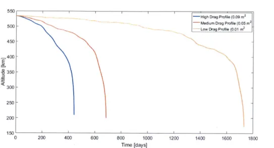
As a perturbation, drag causes secular changes in a, e, and i. It also causes periodic changes in all of the classic orbital elements. Estimating the drag force is important for orbit propagation, but it can also be used as a control force because it is dependent on the area profile of the satellite. Most satellites are asymmetrical, so their attitude can be commanded to change with the goal of adjusting the drag force. This is the basis of differential drag control, which will be discussed further in Section 2.8. Drag effects on the altitude of a LEO CubeSat with different profile areas based on attitude are shown in 2-7. The high-drag area, 0.09 m2, corresponds to the maximum profile area of a 3U CubeSat with single-deployable wing style solar panels, such as the one shown in Figure 2-8, and the minimum area, 0.01 m2, corresponds to

500 450 -400 0350 300 250 200 150 Figure 2-7: 0 200 400

Orbit lifetimes for

600 800 1000 1200 1400 1600

Time [days]

LEO satellites with

1800

different drag profiles

Figure 2-8: The Surrey Training, Research, and Nanosatellite Demonstrator: A 3U CubeSat with single-deployable solar panels [64]

Solar Radiation Pressure

Solar radiation pressure (SRP) is another perturbation, but it is relatively minor for LEO CubeSats. At Earth, the solar flux is often approximated by 1367

y.

High Drag Profile (0.09 m2 Medium Drag Profile (0.05 m

Low Drag Profile (0.01 m2

--h

P = - (2.6)

The force from solar radiation pressure, FSRP, is given by Equation 2.7 where c is the speed of light, 3 x 108 m/s, PSRP = SolarFlux, A is area exposed to the sun, and CR is the reflectivity (varying from 0 to 2) [53]. At 500 km altitude, drag is typically an order of magnitude or more stronger than SRP, but this can vary depending on conditions [12]. As altitude increases and drag becomes less significant, SRP can become the dominant perturbation next to Earth's nonsphericity.

SR _ - PSRPCRA isat

FSRP sat (2.7)

rnTsat

Other Perturbations

Third bodies can also exert perturbing forces on satellites. These effects are most significant for high-altitude satellites and are the cause of phenomena such as the Lagrange points. However, for the purposes of LEO satellites, third body perturbations are small relative to those of drag and Earth's nonsphericity. Tides (both solid and liquid) and magnetic field forces are also perturbations, but they are not considered in this thesis. The major perturbing forces by altitude are shown in Figure 2-9.

0 S-2 -4 _{Lunar gravity} J Solar

gavity

~

1000

Figure 2-9: Effect of disturbing forces by altitude [12]

2.2.3

Gauss's Variational Equations

There are several quantitative ways to describe how perturbations change an orbit. One way is to use the Lagrange's planetary equations. These show the time derivative of each of the orbital elements due to conservative perturbations such as J2. In these equations, R is the negative of disturbing potential. As shown in Table 2.1, J2 is three orders of magnitude stronger than the other spherical harmonics, so it is often the only perturbation considered. Lagrange's planetary equations are shown in Equation

2.8 [53]. 1 I "1 7- 1

~1

da 2

DR

dt

na

_aw

dt

na

dQ

Lagrange's planetary equations are often used for showing how osculating ele-ments, the orbital elements at a single point in time, change over time due to conser-vative perturbations such as Earth's nonsphericity. However, drag is not a conserva-tive force, so Lagrange's planetary equations cannot be used to determine how drag affects orbital elements. For LEO satellites, this is a significant limitation.

Another common way to analyze the effects of perturbations on orbital elements is to use Gauss's Variational Equations (GVE). GVE have an advantage in that they are equally valid for both conservative and nonconservative forces. GVE show the time derivative of each of the orbital elements and how they relate to accelerations on the satellite in the LVLH frame. u, is radial acceleration (pointing away from Earth),

uo is tangential acceleration (pointing in the direction of motion), and Uh is the cross-track acceleration (aligned with the angular momentum vector). GVE use a few intermediate variables related to the orbit. p is the semi-latus rectum, which is half the chord length through the focus of the conic section. b is the semiminor axis. 0 is the argument of latitude. h is the angular momentum, which is the cross product of the position and velocity vectors (r and v, respectively). Gauss's Variational Equations are shown in Equation 2.9 [65].

a

0

e

0

d i 0 0 0 rcos0

- = +UO (2.9)

dtG 0 0 0 "rsin

hsini

Li 0 p cos f (p+r)sin f r sin 6? cos i .

he he hsini

M n b(pcos f-2re) b(p+r) sin f 0

. . _ _ _ ahe ahe

GVE can be used to determine the effect on the orbital elements of a thrust

maneuver on the orbital elements or the effect of some perturbations such as drag. For example, it can be seen that drag mostly acts as an acceleration in the -uo direction, which tends to reduce the semi-major axis. While there are other techniques to describe how perturbations affect spacecraft orbits, GVE are useful for constellations of widely separated spacecraft because GVE are expressed in a curvilinear frame and are linearized about the orbital elements [65]. A curvilinear frame is not necessary for formation flight missions, where satellites are close, within about 100 m, of each other. It is also relatively computationally efficient to express a constellation in terms of classic orbital elements [65].

2.2.4

Mean Orbital Elements

Some orbit definitions are more useful than others for describing relative satellite positions. GPS receivers typically yield position and velocity in the ECEF frame, but position and velocity are hard to use to describe relative motion because they experience large changes on short time scales. The classic orbital elements are more intuitive and useful for describing relative satellite positions when separation distances are large. However, both sets of elements fully describe the state of a satellite, and it is straightforward to convert between them.

Still, because orbital elements constantly change due to perturbations, their defi-nitions can become unclear. Osculating elements are the orbital elements defined at a single point in time. With perturbations, these will vary periodically and secularly. Mean orbital elements are time-averaged to remove periodic effects. Osculating

ele-ments can be averaged over an orbital period to remove short-term effects or over an apsidal rotation to remove long-term terms. For certain applications, the averaging can be important. For example, using orbital elements for constellation management or formation flight, the periodic terms can be wasteful in terms of fuel. Satellites would periodically make corrections due to the short-term periodic variations in or-bital element error. For most applications, this is unnecessary; secular changes are generally the ones that need to be captured. For example, if it is desired that the semi-major axes of two satellites be the same in order to match orbital periods and maintain their angular separation distance, short terms should be omitted because the semi-major axis has large variations over the orbital period. Depending on the exact situation, long terms may also not be desired. The difference between the mean and osculating semi-major axis for a LEO satellite over the course of six months is shown in Figure 2-10. It can be seen that the changes in the osculating semi-major axis are large and have a short period.

Semi-Major Axis

7045

Oscultng Semi-ajor Axis

7040 Mean Semi-Major AxIs

E 7035 7030 7025 6 7020 7015 7010 0 20 40 60 80 100 120 140 160 180 Time (days)

applying them, consistency is important due to differing assumptions for different theories. One technique is Kozai's method, which accounts for the effects of J2 - J5 [66, 53]. Another theory was proposed by Brouwer which uses canonical transformations

to obtain mean elements [67]. Both theories are valid, but their assumptions differ, and different theories should not be mixed [53]. Brouwer's technique is used in this work.

2.2.5

Clohessy-Wiltshire Equations

For satellites in formation flight, which involves multiple satellites working in close proximity in a coordinated effort to accomplish a larger objective, the relative motion of the satellites is often more important than the motion of the group. The close proximity is what differentiates formation flight from other constellations. The Clohessy-Wiltshire (CW) equations, also known as Hill's equations, are often used to describe this relative motion. One satellite is designated as the target (or primary) satellite, and the others are considered interceptor (or secondary) satellites. The LVLH coordinate system, also known as the RSW coordinate system, described in Section 2.2.1 is used. The CW equations are linearized, so the x-axis, y-axis, and z-axis correspond with the R, S, and W axes, respectively. Orbits all exhibit curvilinear motion, but on a small scale (such as below 100 meters), relative positions in the RSW coordinate frame can be approximated as linear. Additionally, the CW equations involve an approximation that is only valid for circular orbits.

Both of these limitations are important. The first approximation means that the equations are not valid for satellites with large separation distances. For a mission involving maximum-separation distances, the CW equations are invalid. Addition-ally, these basic equations assume a circular orbit, though several variations of the equations exist. The equations of relative motion, which have a closed-form solution,. are given in Equations 2.10, 2.11, and 2.12 [53, 68]. The CW equations use the LVLH reference frame, which is shown in Figure 2-11.

= -2ni: (2.11)

-n2z (2.12)

Figure 2-11: LVLH frame of reference (y is in the direction of the velocity vector) [69]

While the CW equations have been shown to be effective for formation flight and rendezvous missions, the necessary approximations make it infeasible for constella-tions where separation distances are large. Relative motion can be better expressed using mean orbital elements in such situations. Additionally, GVE can be used to describe the motion of the spacecraft from perturbations or maneuvers. Although formation flying missions are not uncommon for CubeSats, the majority of multi-nanosatellite missions involve constellations with separation distances over 1 km. [70, 71].

2.3

Propulsion

- One way spacecraft change their orbits is through the use of propulsion systems. The most common systems are cold gas, monopropellant, bipropellant, solid propel-lant, electric propulsion, and ion propulsion. Hot thrusters such as monopropelpropel-lant,

impulse is given in Equation 2.13 where I is total impulse, mp is the mass of the propellant, and g, is acceleration on Earth from gravity. Specific impulse is given in units of seconds. There is a tradeoff between thrust and specific impulse. For example, solid rocket propellant provides a lot of thrust, and this is necessary to get a rocket into space; however, its specific impulse is low. Conversely, ionic propellant tends to provide very little thrust, and it would be unable to get a rocket off the ground, but it is efficient for spacecraft already in space because it has a high specific impulse.

ISp = (2.13)

Including a propulsion system on any satellite has mass, volume, power, and cost impacts. However, for larger satellites, the relative effect of these impacts tends to be less. As discussed in Chapter 1, CubeSats have very strict mass, volume, and power constraints, so many do not fly with a propulsion system.

Several propulsion systems specifically designed for CubeSats exist. Cold gas thrusters are able to provide tens of meters per second of delta-V for a CubeSat

[5, 6, 7, 8, 9]. Electric propulsion systems also exist and can provide up to 100 m/s of

delta-V [6, 9, 11]. Hot monopropellants have also been explored and would provide the most thrust, but they have low I, and the highest power requirements [9, 101. Cold gas and electric systems are more efficient, but they still add complexity and require the use of limited resources. The decision of whether to add a propulsion system or not is far from trivial, and in many cases, CubeSats can perform their mission successfully without it. In situations where relative positions within an orbital plane in LEO must be changed, differential drag can be a viable option. In other situations, such as interplanetary missidns, orbit raising, or orbital plane changes, propulsion is' necessary.

2.4

Global Positioning System

The Global Positioning System (GPS) was introduced briefly in Chapter 1, but this section will focus more on the practicalities of using it and expected performance for small satellites in LEO. In order for a satellite to receive its position and velocity from the GPS, it needs to be receiving information from at least 4 GPS satellites. Three are needed to determine position, and the fourth is needed to obtain precise timing information [54]. GPS signals carry the information necessary for a satellite to determine its position, velocity, and time. Generally these are given in the ECEF frame of reference, but this can be easily converted to other frames, if necessary.

While GPS is often very accurate, there are still errors, and their magnitude can vary in different situations. In high orbits, tropospheric and ionospheric delay of signal can be ignored, but these can still create errors for single-frequency GPS receivers in LEO [72]. However, there also exist errors from inaccurate GPS ephemeris data, multipath effects, superimposed pseudorandom noise, satellite clock errors, and receiver noise [53, 54]. Geometric dilution of precision (GDOP) comes from the

geometry of the user and the GPS satellites. If the GPS satellites are close together from the perspective of the receiver, there will be more GDOP than if the GPS satellites were spread out. GDOP changes the expected error of GPS data.

Global averages on the ground are generally about 2.5, but LEO satellites have been shown to experience GDOP well under 2.0 [54, 72]. On the ground, a common error model uses one-sigma horizontal errors of 10.2 m (horizontal dilution of precision = 2.0) and one-sigma vertical errors of 12.8 (vertical dilution of precision = 2.5). In space, these errors can be expected to be reduced slightly [54]. In this research, position errors were modeled as Gaussian -zero-mean with a one-sigma error of 10 m, and velocity errors can be modeled as Gaussian zero-mean with a one-sigma error of 0.1 m/s [54, 72, 73, 74, 75].