3-D Structural geological models: Concepts, methods, and uncertainties

(1)

HAL Id: hal-01921494

https://hal.univ-lorraine.fr/hal-01921494

Submitted on 23 Aug 2019

HAL is a multi-disciplinary open access

archive for the deposit and dissemination of sci-entific research documents, whether they are pub-lished or not. The documents may come from teaching and research institutions in France or abroad, or from public or private research centers.

L’archive ouverte pluridisciplinaire HAL, est destinée au dépôt et à la diffusion de documents scientifiques de niveau recherche, publiés ou non, émanant des établissements d’enseignement et de recherche français ou étrangers, des laboratoires publics ou privés.

3-D Structural geological models: Concepts, methods,

and uncertainties

Florian Wellmann, Guillaume Caumon

To cite this version:

Florian Wellmann, Guillaume Caumon. 3-D Structural geological models: Concepts, methods, and uncertainties. Cedric Schmelzbach. Advances in Geophysics, 59, Elsevier, pp.1-121, 2018, �10.1016/bs.agph.2018.09.001�. �hal-01921494�

(2)

3-D Structural Geological Models:

Concepts, Methods, and Uncertainties

Florian Wellmann

1

and Guillaume Caumon

2

1

_{Computational Geoscience and Reservoir Engineering (CGRE),}

RWTH Aachen University, Aachen, Germany

2

_{GeoRessources (UMR 7359), ENSG, Universit´e de Lorraine-CNRS,}

Vandoeuvre-l`es-Nancy, France

Authors’ Preprint of Wellmann & Caumon, Advances in Geophysics (2018), Vol. 59, Chap. 1, pp. 1–121, Elsevier. https: // doi. org/ 10. 1016/ bs. agph. 2018. 09. 001 .

NB: Some minor changes exist as compared to the final publisher’s version.

Abstract

The Earth below ground is the subject of interest for many geophysical as well as geological investi-gations. Even though most practitioners would agree that all available information should be used in such an investigation, it is common practice that only a fraction of geological and geophysical information is used. We believe that some reasons for this omission are (a) an incomplete picture of available geological modeling methods, and (b) the problem of the perceived static picture of an inflexible geological representation in an image or geological model.

With this work, we aim to contribute to the problem of subsurface interface detection through (a) the review of state-of-the-art geological modeling methods that allow the consideration of multiple aspects of geological realism in the form of observations, information and knowledge, cast in geometric representations of subsurface structures, and (b) concepts and methods to analyze, quantify, and communicate related uncertainties in these models. We introduce a formulation for geological model representation and interpolation and uncertainty analysis methods with the aim to clarify similarities and differences in the diverse set of approaches that developed in recent years.

We hope that this chapter provides an entry point to recent developments in geological modeling methods, helps researchers in the field to better consider uncertainties, and supports the integra-tion of geological observaintegra-tions and knowledge in geophysical interpretaintegra-tion, modeling and inverse approaches.

Keywords

3-D geometric modeling; spatial interpolation; uncertainty quantification; geological knowledge; joint inversion; complexity;

(3)

1. Introduction and preliminary considerations

“Everything should be as simple as possible, but not simpler”

Albert Einstein (maybe...) The geological space in the subsurface contributes in essential parts to the anthroposphere, as it has a direct influence on mankind and is equally affected by our technological society. Geological processes create significant heterogeneities at multiple scales below the surface of the Earth. These heterogeneities are essential sources of wealth for mankind (e.g., natural resource deposits) but they are also a main driver of natural hazards such as earthquakes and volcanic eruptions. On the other hand, we influence and alter the subsurface geological space, for example due to resource and water extraction, or engineering and geotechnical applications. Therefore, the evaluation of the spatial distribution of properties in the subsurface plays an essential role for a wide range of applications, from scientific investigations, to geotechnical aspects (Culshaw, 2005), hydrogeological investigations (Anderson, 1989), raw materials and hydrocarbons (Ringrose and Bentley, 2015), and finally policy and public hazard information.

Since the first geological map by William Smith more than 200 years ago, geoscientists have put significant efforts in understanding and visualizing how rocks are organized below the Earth surface, both for practical reasons and out of scientific curiosity to understand the world below our feet. This knowledge is now commonly encapsulated in structural geological models, often simply referred to as geological models or geomodels in this context, as a representation of geometric elements such as rock unit boundaries, faults, horizons and intrusions on a scale of meters to kilometers. The goal of this paper is to present recent advances in the field of geological modeling, with interpolation concepts and algorithms that allow us to represent what we do know—and approaches to analyse and quantify uncertainties to clarify what we don’t.

Geological models are intimately linked to geophysics, as they can be seen as a spatial repre-sentation of specific aspects of geological knowledge. In this context, they often provide the basis for a spatial parametrization of geophysical forward models, included in geophysical processing and inversion frameworks. At the same time, geophysical observations and interpretations are often an important input to geological models, and geophysical measurements are commonly used to validate geological models, in combination with petrophysical models.

In our experience, the geometric viewpoint of geological models can provide a link between geolog-ical and geophysgeolog-ical observations with additional geologgeolog-ical and physgeolog-ical information and knowledge, as many relevant aspects share the concept of discrete interfaces in the subsurface as a unifying ele-ment, if only in different forms and appearances. To further explain this idea, we will first describe concepts of interface detection in geophysics and geology and review related work. Subsequently, we will describe the current state of geological modeling methods, specifically with the focus on the potential integration into joint geological-geophysical investigations. Even in the best possible combi-nation of information, uncertainties remain—and a substantial part of recent research addresses the investigation and quantification of uncertainties in geological models. The most relevant aspects are described below, followed by a discussion of the concepts and the major challenges, and an outlook to interesting paths for future work.

1.1. On geological realism considered in structural geological models

The essence of many subsurface investigations is to obtain an estimate of the true physical prop-erty value or class at any location in a region of the subsurface. As we yet have no possibility to directly measure this value exhaustively in space, we need to combine all available measurements, observations, and knowledge to obtain an informed estimate for it.

(5)

Of course, the spatial distribution of properties in the subsurface is not random—it is rather the result of the highly complex and long geological history that finally led to the state of the system that we observe in its present form. Unfortunately, we cannot model the entire evolution of the Earth in such a detail that we would be able to obtain a completely realistic picture of the spatial distribution of all relevant properties. Instead, we aim to formulate models that capture essential aspects of this evolution, which we deem relevant for the purpose and scale of a specific investigation. This specific consideration of geological knowledge can be considered as geologic realism, and an essential question for each subsurface investigation is: which type of geological knowledge and how much geologic realism is required for a specific modeling aim and purpose?

In this manuscript, we focus on geologic realism with respect to dominant structural geometric features. The motivation for the consideration of these features is best described with an image of a geological structure, provided in the following section.

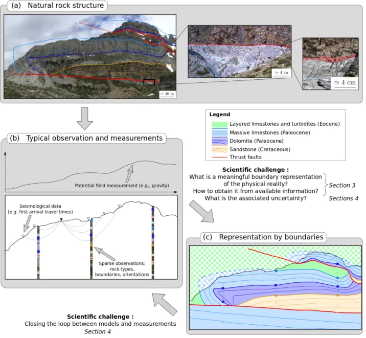
1.1.1. A natural rock structure as a motivating example

We take here an example of a folded carbonate layer in the Pyrenees (Aragon, Spain), presented in Fig. 1a. The (simplified) geological story on the area associates sedimentary and tectonic processes (Alonso and Teixell, 1992): during the Upper Cretaceous, sandstone (Marbor´e Formation) was deposited on top of the Pyrenean basement rocks, and was then overlaid during Paleocene by dolomite and massive limestone beds. Layered carbonate beds were deposited during the lower Eocene, then a sudden rise of the relative sea level led to the deposition of deep-marine turbidites of the Hecho Group. This sea-level rise is explained by a fast subsidence related to the Pyrenean compression which provoked a flexure of the lithosphere on either sides of the axial (collision) zone. The North/South shortening then affected these sediments, which accommodated deformation by folding and faulting. This history is inferred from observations by applying basic stratigraphic principles established in the seventeenth century Steno (1669): more recent strata are deposited roughly horizontally on top of older strata; variants stem from later geological events. Geological concepts have much evolved since then, but these essential principles are still applicable in general.

Clearly, we cannot capture the entire complex history quantitatively, including the formation of the basement, the details of erosion and sediment transport and marine life which lead to the formation of sediments, global and regional effects like sea-level rises and subsidence, and finally the complexities of the Pyrenean orogeny. However, what we choose to consider when we talk about structural geological models are surfaces in 3-D space, which capture the essence of geological events in this complicated and long history and which are often manifested at discrete points in time1. These surfaces are, for example, related to changes in the depositional system, leading to different rock types that we observe today, or related to deformation events like faulting or ductile deformation2

If we now consider the realistic case that we can not observe the geological domain in an out-crop in the Pyrenees, but that it may be several meters to kilometers below the surface, then the next question is how this geometric representation can be obtained from only a limited amount of information that we typically have (Fig. 1b): boreholes may provide direct observations, but only at very limited points in space, and geophysical measurements provide additional indirect information. How can we “join the dots”, considering all of this partial information, and equally use the aspect of geologic realism that we described above?

The fundamental goal for the theory of geological modeling is to obtain methods that allow a reasonable description of geometric and topological features in full 3-D space (Fig. 1c). As all models, this description is bound to approximate the truth within some tolerance. For example,

1_{Discrete in the sense of very short, in a geological time frame.}

2_{Note that this explanation is mostly for sedimentary systems, but equal considerations and thoughts can}

lead to structural models of poly-deformed magmatic and metamorphic rocks (e.g. Calcagno et al., 2008; Maxelon et al., 2009), or even unconsolidated rocks and soil systems.

(6)

Figure 1: Example of complex geological structures as seen on outcrop (a): this fault-related fold involves juxtaposition of sharp boundaries between turbidites, carbonates, and sandstone. As typical observations are incomplete and sparse (b), a challenge is to decide on which boundaries to represent, and to determine their geometry con-sistently with conceptual knowledge and the associated interpretations. Location: Aragues del Puerto, Aragon, Spain.

details on the right of Fig. 1a showing some internal structures, joints and details about the fault core zone, may be consciously ignored and deemed impractical to represent explicitly at the scale of interest. The construction of a geological model is limited by the ability of the selected methods to represent the level of geological realism that is considered on a specific scale. The geological models presented here often act as the framework models for models of finer-scale variability, for example using geostatistical approaches (e.g. Pyrcz and Deutsch, 2014b; Ringrose and Bentley, 2015). Geological models are therefore often hierarchical models, combining multiple scales. Even though we limit our exposure here to structural models, we will mention this link at appropriate positions in the paper and highlight its relevance in the discussion.

(7)

is illustrated by some differences between the reality on Fig. 1a and the model on Fig. 1c: Surfaces are locally smoother in the model, and a small fault visible in the outcrop is missing in the model. As a combined result of limited precision, conceptual and observation limitations, each geometric representation will be uncertain. An increasing amount of recent research is going into the evaluation of these related uncertainties.

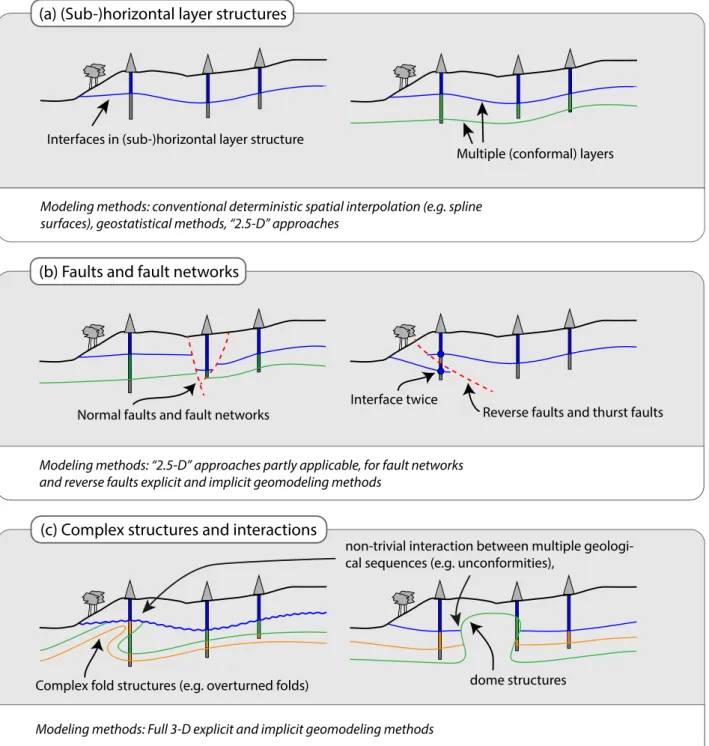
1.1.2. A note on model complexity

An important aspect of geologic realism is the question of complexity of the investigated geological setting, and specifically, how much of this complexity should be represented in a subsequent geological model. We refer here with geological complexity purely to the complexity related to the geometric setting, in line with the purpose of this paper, (see also Wellmann et al., 2010a; Jessell et al., 2014; Pellerin et al., 2015, for more details on this consideration). Typical levels of complexity that we will consider are sketched in Fig. 2, and concern the number of geological features of interest (e.g., number of geological interfaces or contacts between interfaces), and the possible relationships between these features.

The simplest possible structural elements in geological models are continuous sub-horizontal in-terfaces (Fig. 2a): at each location (x, y) in the model domain, this interface has exactly one cor-responding z value as a function of this location, z = f (x, y). We refer to these methods here as map-based3. This type of structure can be modeled with a wide range of existing interpolation techniques, including geostatistical approaches. The situation is slightly more complex for multiple conformal layers (Fig. 2a, right), as the relationship between layers has to be considered (e.g. layers should not cross, constraints on thickness variations), but techniques for these elements also have long been available (e.g. Abrahamsen, 1993). More details are provided in Sec. 3.2.1.

The modeling situation is more complex when faults and fault networks are considered (Fig. 2b). First, faults add additional geometric elements that need to be modeled. Furthermore, geological continuity across faults often has to be taken into account, as faults act as discontinuities in the geometric sense and lead to a significant increase in topological complexity (e.g. Pellerin et al., 2015; Thiele et al., 2016a). And finally, reverse faults (Fig. 2b, right) also increase the complexity for a geological layer, as they lead to a layer doubling, resulting in the interface potentially existing twice at a single location (x, y) in space, making map-based interpolation methods unsuitable.

A high level of complexity in both geology and topology is also quickly reached when more com-plex poly-deformed terranes and the interaction between geological sequences is taken into account (Fig. 2c), for example due to the consideration of several cycles of sedimentary sequences and un-conformities. Other examples are intrusions and dykes in a region. Furthermore, overturned folds lead to interface doubling, similar to reverse faults. The same is true for dome structures (Fig. 2c, right).

Overall, faults, fault networks and deformation or intrusion settings quickly add a level of com-plexity that many conventional interpolation algorithms can not consider and thus call for dedicated full 3-D geological modeling techniques. These methods will be further discussed in Sec. 3.1.3 for explicit approaches, and Sec. 3.2.3 for implicit approaches.

This consideration of the required level of geological complexity is very important, as it is strongly linked to the selection of a suitable modeling algorithm (discussed in Sec. 3), and the possibility to analyze model uncertainties (Sec. 4). It is also an aspect where most geophysical subsurface investigations diverge from more geologically-oriented approaches. This distinction is explained in more detail in the following section.

3 _{Similar in the level of complexity are extrusion (or “2.5-D”) approaches which assume that geological}

(8)

(a) (Sub-)horizontal layer structures

(b) Faults and fault networks

(c) Complex structures and interactions

Modeling methods: conventional deterministic spatial interpolation (e.g. spline surfaces), geostatistical methods, “2.5-D” approaches

Modeling methods: “2.5-D” approaches partly applicable, for fault networks and reverse faults explicit and implicit geomodeling methods

Modeling methods: Full 3-D explicit and implicit geomodeling methods

Interfaces in (sub-)horizontal layer structure

Multiple (conformal) layers

Normal faults and fault networks Reverse faults and thurst faults

Complex fold structures (e.g. overturned folds)

non-trivial interaction between multiple geologi-cal sequences (e.g. unconformities),

dome structures Interface twice

Figure 2: Complexity from the viewpoint of structural geological modeling: different geological settings and possible geomodeling approaches

1.2. Two viewpoints on interface detection

The problem of interface detection has occupied geophysicists and geologists for a long time. Ar-guably, two different viewpoints on this problem have emerged in this context: an approach to detect interfaces on the basis of geophysical data and measurements, described as the data-driven approach below, and an approach on the basis of geological observations and considerations, referred to as a geomodel-driven approach in the following. This contrast in the view on the same problem po-tentially derives from the academic background and language, and both approaches take different

(9)

assumptions, but also share many commonalities.

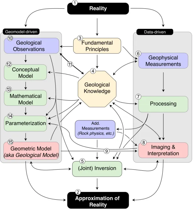
The essential aspects of both viewpoints are presented in Fig. 3 and we will develop our interpre-tation on these viewpoints in the following and especially illustrate how they interact. For clarity, encircled numbers are added in the following text (e.g. 3) to refer to positions in Fig. 3. We aim to provide an overview of different aspects related to geological modeling and the link to geophysics, but also hope to provide a framework which can be helpful to place the great body of existing work, or new approaches in this field, into context, and to detect potentially interesting links to related work.

Both viewpoints initiate from the same object of interest: the physical reality 1 of the subsur-face. As we cannot directly measure this reality in a comprehensive way, we combine models of measurements of different types with mathematical and numerical models to finally arrive at an ap-proximation of reality, 2. Both paths are linked in multiple ways and share several commonalities. They are both based on fundamental principles 3, for example physical laws, and also on geological principles. In the following description, we aim to specifically examine the role of geological knowl-edge 4 and highlight the role of joint inversion methods 5 as a way to combine geological and geophysical information in a principled way.

1.2.1. The data-driven approach

We first describe the data-driven approach to obtain an approximation of reality on the basis of geophysical measurements 5. The commonly expressed aim is then to obtain a subsurface model 2 of interfaces or directly property distributions from this data. A great body of work has been performed in this field, and multiple methods are now available and used in scientific investigations and practical applications with specific considerations for each geophysical measurement type. We will limit the following description to a general overview and provide some references to relevant literature with more details.

All geophysical data-driven approaches logically start with geophysical measurements 6. These measurement may have been taken for a specific purpose (as often the case in targeted exploration, for example), or as a general regional measurement (as, for example, magnetic and gravity state-or country-wide surveys). The measurements themselves are often derived from basic physical prin-ciples, but depending on the origin and type of measurement, geological knowledge 4 may have been considered for the measurements themselves, for example in the design of a survey. A typical example is the decision about a suitable trace for a 2-D seismic or gravitational survey, perpendicular to the strike of the investigated geological structures (e.g. Yilmaz, 2001; Telford et al., 2009). At the same time, geophysical measurements can be used to derive first insights into the subsurface. An experienced applied geophysicist may be able to directly interpret measured signals, for example raw gravity or magnetic measurements to obtain a first insight into subsurface structures. Geophys-ical measurements themselves can already contribute to a general geologGeophys-ical knowledge of a specific region.

Still, the main contribution of geophysical measurements is usually obtained after dedicated data processing 7. Examples are the various steps in seismic processing from raw data processing and stacking, over migration, to time-depth conversion to obtain a reflection image (e.g. Yilmaz, 2001), or the various corrections applied to potential-field data (e.g. Telford et al., 2009; Jacoby and Smilde, 2009).

Geological knowledge may also enter the processing workflow at this stage, for example in the form of bounds for velocity models for migration in seismic processing. An example for the use of geological reasoning in the analysis of potential-field data are also the various signal processing methods, which are often based on physical principles (for example considering the upward continuation of wavelengths of gravity anomalies), but may also directly consider geological interfaces as the main object of interest, for example when using wavelet-based methods (e.g. Hornby et al., 1999).

(10)

Reality

Approximation of

Reality

Geological

Observations

Geophysical

Measurements

Fundamental

Principles

Processing

Imaging &

Interpretation

Conceptual

Model

Mathematical

Model

Parameterization

Geometric Model

(aka Geological Model)

Add. Measurements

(Rock physics, etc.)

Geological

Knowledge

(Joint) Inversion

Data-driven Geomodel-driven 1 3 4 6 5 2 7 9 12 11 10 8 13 14 15

Figure 3: Two viewpoints on subsurface interface and property detection; blue boxes: mea-surements and observations, green boxes: processing and modeling steps, red boxes: intermediate representations, yellow boxes: fundamental principles and knowledge. The circled numbers and letters refer to important aspects and links, explained in more detail in the text.

(11)

seismic data makes it possible to estimate a velocity model of the subsurface and to produce seismic images with limited geological information. In this case, the common approach is to use smoothness constraints in the regularization method; whereas it may be a suitable approach to consider smoothly varying velocities under the Born approximation, many aspects of geology can not be considered in this way, because major and significant changes between subsurface areas with distinctively different properties appear on many sharp boundaries at multiple scales, as obvious in outcrops and rock-faces in nature (Figure 1a).

From processed data, two paths can be taken: the first is a direct interpretation of the processed data 8, and the second a further combination with additional mathematical methods in an inversion framework 5. In the first case, the aim is to produce a geophysical image, for example a profile of reflection seismic, or a spatially interpolated map of processed potential-field measurements at the surface, also then often called a geophysical map (e.g. Jacoby and Smilde, 2009; Dentith and Mudge, 2014). In this step, the geophysical measurements are necessarily combined with geological knowledge in order to derive a meaningful interpretation (e.g. Saltus and Blakely, 2011). In a minimal form, the concept of interfaces is used in the interpretation step, as obvious in the detection of interfaces on reflection seismic images (e.g. Yilmaz, 2001), or lineaments on gravity maps (e.g. Dentith and Mudge, 2014). However, there is also a significant contribution of more expressive forms of geological knowledge in this step. For example, in the case of seismic interpretation, Bond et al. (2007) and Bond et al. (2012) showed the significant influence of prior geological knowledge about a region on the interpretation of structures from seismic images. Even in the case of relatively well-constrained geological knowledge, uncertainties may exist in the location of the number, the geometry and the connectivity of faults.

In addition to geological concepts, geological models often inform the interpretation step of geo-physical data. The most obvious link is in the form of geogeo-physical forward models, which are based on property distributions assigned to regions in a geological model, for example a model of gravity response at the surface from defined mass distributions in the subsurface (e.g. Jacoby and Smilde, 2009).

Finally, interpreted images or geophysical maps are already often an end-point in the data-driven workflow and taken as a suitable approximation of reality 2 for a specific purpose. At the same time, the additional understanding during the intellectual process of geophysical image and map interpretation also feeds back into the general geological knowledge about a specific region.

We now consider the second path from processed geophysical measurements 4 to final models 6 using inversion approaches 5. We aim here to specifically outline the link of various inversion approaches to geological knowledge 3, specifically with the link to the geometric mode of interface detection.

Typical inputs to inversion approaches are based on either directly using the processed geophysical measurements 7, or already results from the imaging and interpretation step 8. A direct combi-nation exists in the inversion of interfaces from gravity and magnetic data (e.g. Silva et al., 2001; Jacoby and Smilde, 2009). The non-uniqueness of the inverse problem to determine density distri-butions from these measurements has been the content of early research in the field of geophysics (e.g. Parker, 1974), and subsequent work on suitable constraints for inversion (e.g. Li and Oldenburg, 1998). Geological knowledge 4 , potentially also derived directly from geological measurements, has, for example, been considered in the form of dip measurements (e.g. Li and Oldenburg, 2000; Leli`evre et al., 2012). Many approaches also exist to invert density or velocity distributions or interface po-sitions from a geological starting model (e.g. Bosch, 1999; Bosch et al., 2001; Fullagar et al., 2008; Guillen et al., 2008; Joly et al., 2009; Schmidt et al., 2011; Gradmann et al., 2013; Autin et al., 2016; Haase et al., 2017; Zheglova et al., 2018b). The direct link to the geological model itself 9 is here very obvious.

Similar approaches exist for the inversion of electric and electromagnetic data, as well as seismic data (e.g. Guiziou et al., 1996; Clapp et al., 2004; Hauser et al., 2011, 2015) In fact, the relevance of boundaries has also long been realised as a central aspect of geophysical imaging techniques

(12)

and a lot of work has gone in this direction since the pioneering work of Gjøystdal et al. (1985). However, several studies explicitly suggested that geological insight can help seismic interpretations (e.g., Rankey and Mitchell, 2003; Osypov et al., 2013) and that, even when using modern seismic acquisition and processing practices, there is still ambiguity in velocity models that can lead to significant uncertainties in the true position of events in images. Very interesting is the also increasing research on full waveform inversion of seismic data (e.g. Kamei and Lumley, 2017; Zhu et al., 2016). These approaches can certainly be considered as dominantly data-driven, however non-uniquenesses still remain and the inversion results depends on an initial (or baseline) velocity model.

As a summary of the data-driven viewpoint based on geophysical measurements 6 to obtain an approximation of reality 2, we see that a lot of work is aimed at a quantitative and, as much as possible, data-driven and mathematical analysis of the obtained measurement data. However, there is the fundamental problem that the measured geophysical signals provide only an indirect measure of the subsurface interfaces and properties, and an infinite-dimensional manifold of solutions exists (Backus and Gilbert, 1967; Parker, 1974). From a mathematical point of view, this ambiguity leads to ill-posed problems, and these have to be addressed with suitable regularization methods (e.g. Tikhonov, 1963; Aster et al., 2005). In fact, the ill-posed nature of geophysical problems lead to many of the mathematical developments in this field (e.g. Kabanikhin, 2008). In order to obtain non-unique and meaningful solutions, many decisions have to be taken, beginning from suitable regularization methods, to processing steps and the consideration of additional information in the form of geological models or constraints. There exists, therefore, no completely objective result for the inversion of geophysical data.

Many (if not all) of the steps in the “data-driven” approach therefore contain at least some as-pects of geological knowledge. Several authors explicitly state that geological considerations increase the effectiveness of geophysical inversion (e.g. Fullagar et al., 2008). The fundamental question is therefore how this geological knowledge is obtained—and how relevant parts can be implemented at suitable steps in this “data-driven” viewpoint. These aspects are best explained in the framework of the “geomodel-driven” viewpoint, described below.

1.2.2. The geomodel-driven approach

A different point of view, anchored on centuries of work in the field of geological investigations, is to initiate the subsurface investigation from the viewpoint of main geological interfaces and the related primary information, as well as the associated geological concepts. This way of thinking is underlying the concept of geological maps and has subsequently been extended to full 3-D geological models. This viewpoint is at the core of understanding the relevant steps of geological model construction and the related uncertainties, and all essential aspects will be described in more detail in subsequent sections of this manuscript.

In this viewpoint, primary data are geological observations and measurements, for example in outcrops or wells 10. Here, the link between observations and geological knowledge 11 becomes essential and deserves a specific note: geological observations can never be separated from geological knowledge. Even taking a measurement of a surface orientation in an outcrop requires the previous geological knowledge about the interpretation of relevance for a feature, or the detection of a fault plane. This realization is at the core of the hermeneutic aspect of geology (e.g. Frodeman, 1995) and described in more detail below.

The set of observations, combined with the purpose of the model and the geological knowledge, typically first enter into a conceptual model 12. This conceptual model should consider all geological elements and available information, as well as aspects of geological knowledge with relevance for a specific study. This conceptual model is then the basis for the decision on an appropriate mathe-matical model for the geometrical interpolation in space 13. Typical interpolation functions and the associated assumptions and limitations are described in detail in Sec. 3. We note here that this decision is also based on the question of geological realism to be considered and, most importantly,

(13)

on the level of complexity.

Once the representation and associated interpolation methods are defined in the form of a math-ematical model, we can assign geological observations as parameters to this model 14. This step includes the definition of all relevant geological elements, as well as their interaction, for example the number of layer interfaces, and the structure of a fault network. This decision is clearly influenced by the conceptual model, geological measurements and the amount of available information, but, it is also often limited in practice by the specific mathematical model that is applied. The choice of a specific type of model representation and geological interpolation function determines which data can be used—and which can not.

The most commonly used geological observation type is interface points (e.g., Hardy, 1971; Dubrule, 1984; Mallet, 1992), but the direct integration of orientation measurements is only possible in a few interpolation algorithms (e.g., Lajaunie et al., 1997; Hillier et al., 2014; Frank et al., 2007). We specifically note that the set of geological input parameters can also contain drawings of interfaces in cross-sections, generated by a geological expert, or more subjective knowledge conveyed through interpretive interface points. Yet again, other interpolation methods can consider thickness informa-tion (for example kinematic algorithms, Jessell, 1981; Wellmann et al., 2016).

Next to direct geological observations and measurements, interpreted geophysical images and sections 8 are commonly used as an input to the parametrization of interpolation functions. Typical examples are reflection seismic data and geophysical maps of potential-field data. In many cases, this information enters directly into the interpolation step (e.g. interface picks in a seismic section), in other cases, it is included through the intermediate step of geological knowledge in a region, which is often informed by the consultation of all available geophysical images and interpretations and then considered in the definition of the conceptual model 12 and the choice of the mathematical model

13, as well as the parametrization of the interpolation functions 14.

In addition to the parameters based on geological and geophysical observations and measurements, each interpolation function requires specific parameters. These parameters are sometimes estimated on the basis of observations (e.g. parameters of covariance functions in geostatistical interpolations), but often based on a general expected behavior (e.g. smoothness of the interface). In addition, we often need to consider multiple interpolation functions to represent different geological sequences and structures, and then also have to define the interaction of these functions. More details on typically used mathematical interpolation functions and model parametrization are presented in Sec. 3.

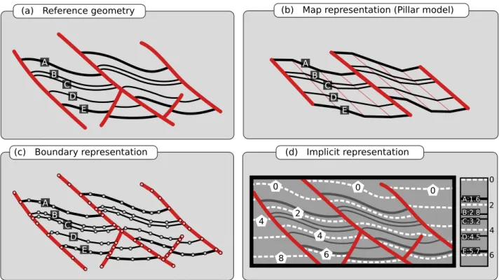
Once interpolation function(s) and parameters are defined, we obtain a geometric representation of the defined geological features in space. The most common example today are full 3-D visualizations, either of surfaces as boundary representations, or volume models on discretized mesh structures (e.g. Caumon et al., 2009), and these 3-D representations are often referred to as structural geological models or simply geological models4. We note, however, that 2-D sections are also a common repre-sentation, also in the form of a geological map, as the intersection between a 3-D geometric model and a digital elevation model.

The geometric model 15 is then an important aspect of the required approximation of reality 2. Other common aspects include property fields with additional rock property models, possibly also in combination with further small-scale models of spatial heterogeneity to represent variability on a scale below the considered structures (see Fig. 1).

In any case, given all aspects considered before, it is already obvious that geological models can contain several sources of uncertainty, starting from the initial geological observations, over potentially vague and subjective aspects of geological knowledge, to the choice of the mathematical interpolation approach, its geometric and topological structure, and any additional interpolation parameters. In addition, we also observe that the diverse set of input data and the required choices in the model construction step also lead to different types of uncertainty, for example uncertainties

4_{The term geological model is, of course, highly ambiguous and should only be used when the context and}

(14)

that are related to fixed choices made by the modeling expert in the definition of the conceptual model, different interpretations of features on a geophysical image, or measurement uncertainties in primary data. The treatment of these uncertainties is therefore closely linked to different steps in the geomodel-driven viewpoint and the respective choices in each step. The different sources and types of uncertainty are further discussed in Sec. 2.

It is clear from the description above that the geological model or map is, in essence, only a representation of one or several interpolation function(s) and the defined parameters, even though this aspect is often obscured by the fact that geological modeling methods are often hidden behind “black-box” implementations in commercial software packages. This understanding will, however, become essential for the treatment of diverse aspects of uncertainty, as many methods require the possibility for an automatic update of the geological model. From the previous description, it is evident that this level of automation is generally possible when the choices and settings in the mathematical model 13 and the parametrization 14 are made transparent.

This automation opens the way to an estimation of uncertainties in geological models. This is a key aspect of recent research in this field, and methods to estimate, quantify and visualize the effect of these uncertainties on the subsequent geological models are treated in Sec. 4. An important point to mention here is that this automation allows for a tight integration of the geological modeling step into inversion approaches. This feature is relevant as it allows, for example, the consideration of geological observations and general aspects of geological knowledge that can not directly be integrated into the geological (forward) modeling step. In addition, it provides the possibility for a tight integration with geophysical measurements, through the use of geological models in joint inverse approaches 5. The basis for this integration is typically a geophysical forward simulation on the basis of the spatial distribution of rock properties, obtained from the geological model.

1.2.3. Combining elements

The separation into two distinct approaches is clearly a simplification, but it captures the two main viewpoints on this problem and it is also, in our experience, the cause for a lot of misunderstanding between researchers trained in different fields. Both approaches have strengths and weaknesses. However, we specifically want to highlight here the links and the high connectivity between these different viewpoints, as described above and illustrated in Fig. 3.

Two important links exist between both viewpoints and can address the above concerns: (a) the central aspect of geological knowledge, and (b) integrated inverse approaches. Both aspects are directly related: the underlying geological reality is the combining element between all types of investigations, and our knowledge about it is therefore a central aspect, whereas integrated inverse approaches include the technical possibilities to obtain a model of the reality under the consideration of all available and relevant information.

A central problem with geological knowledge, though, it that it is very difficult to express in a quantitative and objective way. This aspect is fundamentally related to the fact that geological observations themselves can not be taken without a framework of knowledge, as already described above. We can instruct someone how to measure a planar feature with a geological compass, but if we place this person into an outcrop, he or she will be completely lost without the knowledge of how to identify a meaningful planar feature to measure5. This aspect is encapsulated in the characterization of geology as a hermeneutic science with a strong interpretative character Frodeman (1995) and it leads to the fact that many geological observations have a subjective character. This is very different with many geophysical measurements, which can technically be taken (although certainly not interpreted) without any knowledge about the subsurface, purely on the basis of the

5_{To some extent, this is not true for all possible measurements. For example, it is possible to identify grain}

sizes on a core sample without knowing details about sedimentology. This is why geologists often have several terms to describe the same reality: some terms are mainly descriptive, while some others bear also an interpretation sense.

(15)

measurement technique itself. For example, gravity measurements can be performed by experienced technicians. This is certainly a generalization, but overall a significant difference between geological and geophysical measurements and observations.

To re-state this aspect in our context of subsurface investigations: we cannot deny the ubiquity of interpretative and subjective aspects—but we can find ways to address this subjectivity. One approach addresses the elicitation of knowledge from experts as an attempt to reduce subjectivity in primary information (e.g. Curtis, 2012). A complementary approach is to find ways to reduce the effect of this uncertainty through the use of all available information—and to achieve this aim, we need to combine both viewpoints in the best possible way.

In the end, we obtain then the approximation of reality 2, informed by the geometric represen-tation of the geological model and potentially optimized with additional geophysical information. As a result of the early integration of geological concepts and the tight link to geological knowl-edge, geomodels may include not only features directly visible on the geophysical data at hand, but also features that are expected on the basis of related prior geological information (e.g. sub-seismic fracture networks). This concept is also commonly known as “Shared Earth Model” in the petroleum industry (Gawith and Gutteridge, 1996), or “Common Earth Model” in the mining in-dustry (McGaughey, 2006b). Concrete examples of this approach to real-world problems have also been proposed in other fields such as geodynamics (e.g., Ziesch et al., 2015), seismology (e.g., Shaw et al., 2015) and geological engineering (e.g., Kaufmann and Martin, 2008).

The previous exposure does not answer the question of the required level of complexity for a specific study. As all modeling assumptions, this aspect requires the consideration of the specific model purpose. The geomodel-driven approach, therefore, should certainly not be confused with simply adding all detail and complexity that is present in nature, to obtain a “realistic” picture. The aim of modeling is always an abstraction, and this consideration holds here in the same way as in other cases (see also discussions in Ringrose and Bentley (2015); Caumon (2018) and throughout this paper).

1.3. Typical input data

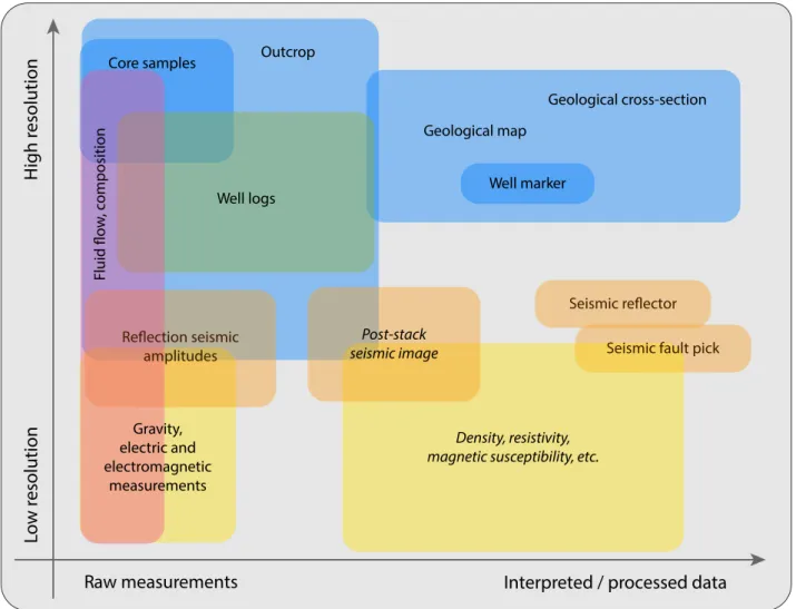
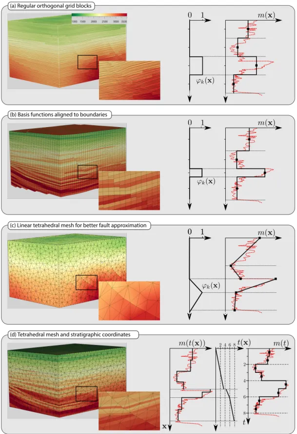
Three-dimensional geological modeling generally starts with spatial points, lines or surfaces inter-preted from available observations and measurements. The data used in geomodeling is very het-erogeneous and includes direct observations of rocks and indirect geophysical measurements. The heterogeneity of data is in itself a challenge in geomodeling: gathering all relevant information can take significant time due to accessibility and numerical storage issues. Another challenge is to assess the reliability of this information, as several sources of uncertainty affect these geoscientific data: position of the measurement, accuracy of the measurement device, volume being investigated. The quantity of interest (e.g., magnetic susceptibility) may also not directly relate to the feature to be modeled. As direct accessibility is limited to the Earth surface and to boreholes and galleries, spatial representativeness of Earth data is also very important. These limitations imply varying degrees of processing and interpretation even before three-dimensional modeling starts. Fig. 4 show some typical types of earth data used in geomodeling, classified according to their volume of investigation and to the degree of interpretation they carry.

More precisely, geomodeling applications typically use several data types (e.g., Kelk, 1992; Kauf-mann and Martin, 2008; Ringrose and Bentley, 2015):

• Surface data include pictures and other remote sensing data (which may be combined into digital outcroop models), textual descriptions and drawings, georeferenced structural ob-servations and measurements describing lithology, stratigraphy, unconformity, fault, strati-graphic orientation, fault striae, etc. These data are typically used directly as input for three-dimensional modeling, but are often initially translated into maps and cross-sections.

(16)

Raw measurements Interpreted / processed data Lo w r esolution H igh r esolution Seismic reflector Seismic fault pick

Geological map Geological cross-section Well marker Well logs Outcrop Core samples Reflection seismic amplitudes Post-stack seismic image Gravity, electric and electromagnetic measurements Fluid flo w , c omposition Density, resistivity, magnetic susceptibility, etc.

Figure 4: Typical Earth data used in geomodeling. All data relate to a range of spatial res-olution (vertical axis), and imply varying degrees of processing and interpretation (horizontal axis). Only a few data types (in italic) provide exhaustive spatial cov-erage in three dimensions. Colors highlight the type of data for various levels of processing and interpretation.

• Geological maps and cross-sections result from two-dimensional interpretations filling the gaps between surface observations. The reliability of this information essentially depends on the distance to actual observations and on the interpreter’s skills, which are seldom ob-jectively documented. In practice, 3-D visualization and modeling can help improving these interpretations by allowing the interpreter to consistently map in space.

• Borehole data include both well cores and geophysical well logs. Cores have the same features as surface data, but may be more difficult to interpret, as no rocks are generally observed away from the borehole. Geophysical logs are typically images or result from a local geophysical measurement which reflect physical properties in the neighborhood of the well. Images logs may contain significant structural information to identify layer dips and fractures. Overall, borehole data tend to be sparse and may have representativeness problems, as their location is often geared towards natural resources. The borehole data are generally interpreted in terms of location or range of location for the various geological surfaces.

(17)

dimensional image. Reflection seismic data particular provide extremely useful information to identify reflectors and the associated discontinuities, which are then interpreted in terms of geological objects (e.g. Jacoby and Smilde, 2009). Depending on the type of the geophysical method, on the quality and on the spatial coverage of the data, interpretations may bear a variable value in resolving geophysical ambiguities.

• Flow data include flow rates at wells, transient pressure/ height and fluid composition mea-surements. This type of data does not explicitly include geological information, but can indi-rectly tell a lot about how subsurface reservoir rocks are connected.

Finally, if we neglect interpretation uncertainties, most geomodeling input data end up as labeled points indicating the most likely location and/or orientation of a particular geological surface. Ad-ditionally, we often have access to interval data (indicating the presence or absence of a particular geological feature in some region of space, a common case in geological field campaigns, for example) and trend data (indicating the slope, the fold axis or the dip and dip direction of geological inter-faces). Additional information may also be used as input data, for instance the fault displacement or the thickness of a particular stratigraphic layer (Mallet, 1992), or may be considered as a way to (in)validate a generated model (e.g. de la Varga and Wellmann, 2016).

After the general overview of the considered aspects of geological realism, the conventional work-flow with links to geophysics, and the typically used input data and the link to geological knowledge, we now consider the very opposite: the lack of precise knowledge about the subsurface, and the sources and types of uncertainty in geological models.

(18)

2. Classification and origin of uncertainties in Geological

Models

“[...] you cannot do inference without making assumptions”

David J. C. MacKay Uncertainties have been an integral aspect of geological investigations since the early days of mining and exploration. This uncertainty is enshrined in common sayings between miners (“All is dark ahead of the pick”6), but it is just as well recognized for the oldest form of geological models, geological maps, where it has always been common to highlight uncertain areas and interface continuations, for example using dashed lines or different line thicknesses and shading (e.g. Greenly, 1930).

A notable increase in research around uncertainties in geological maps and models occurred in relation to the development of digital mapping and modeling techniques. Early developments are represented in the work of Mann (1993), and the excellent review by Jones et al. (2004) about uncertainties in geological mapping and modeling. In the latter paper, the authors describe the relevance of different types of geological knowledge (see also Sec. 1.2 and Fig. 3) and link these types of knowledge to different typical observations during geological mapping (see table 4 in Jones et al., 2004). These classification approaches were oriented along descriptive aspects, related to the process of data gathering and model building.

Similar considerations can be made for the typical workflow of geological model construction described above (Sec. 1.2.2). At each step in this modeling process, important decisions have to be taken, partly based on limited information and general aspects of geological knowledge, as well as measurements and observations, all subject to uncertainties. All of these decisions will manifest themselves in the final model (and, logically, also in the approximation of reality) in the form of model uncertainties.

In this section, we first describe sources of uncertainty related to each modeling step. We then provide an overview of uncertainties of typical input data. Finally, we describe approaches to classify uncertainties and propose a terminology based on uncertainty quantification concepts.

2.1. Uncertainty in the context of model construction

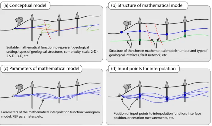
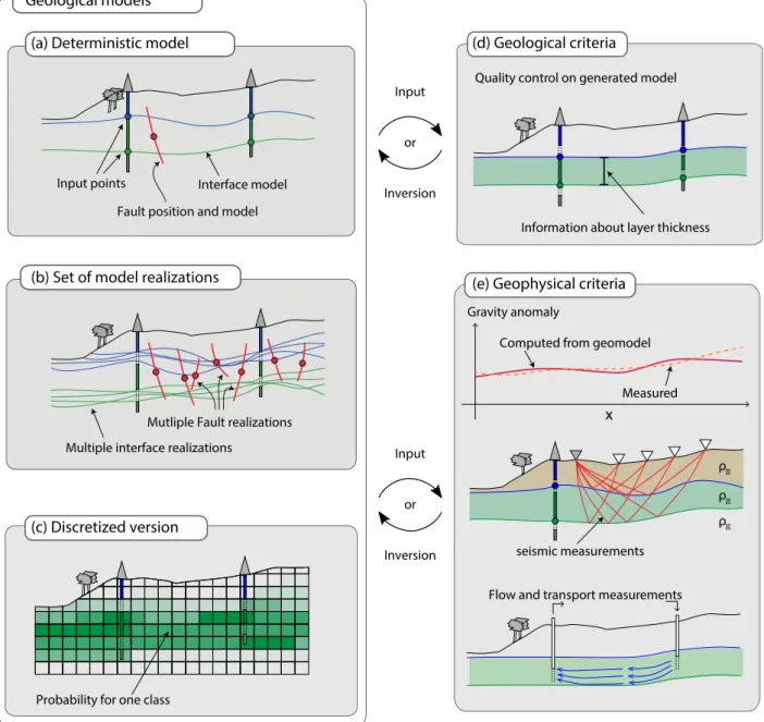
If we consider the workflow of model construction (Sec. 1.2.2, Fig. 3), then uncertainties enter at several levels: (a) at the definition of the conceptual model and the decision of the mathematical model, (b) at the definition of the structure of the mathematical model, (c) when selecting parameter values for the mathematical model, and finally (d) at the the exact value of the measurements. These steps and related uncertainties are presented in Fig. 5.

If we start from the model construction phase (Sec. 1.1), we first define a conceptual model, and here uncertainties are related to the lack of geological knowledge. This step is also heavily influenced by personal experience and belief (e.g. Frodeman, 1995; Bardossy and Fodor, 2004; Bond et al., 2007). On this basis, we decide on the mathematical model to perform the modeling step (described in more detail below, Sec. 3.2). We now need to decide on the structure of the model itself, for example how many layers to include and how many faults. This step is closely related to the conceptual model, but we emphasize that it is not necessarily the same: a typical example would be the case where the exact number of layers is uncertain, and we would like to evaluate it from data. Examples will be given below. At this stage, the model space contains all of the models that are possible on the basis of the mathematical model and the defined structure. Finally, we consider the data itself and we only keep the models which actually explain the observed data, given the measurement uncertainties.

(19)

(a) Conceptual model

Suitable mathematical function to represent geological setting, types of geological structures, complexity, scale, 2-D - 2.5-D - 3-D, etc.

(b) Structure of mathematical model

Structure of the chosen mathematical model: number and type of geological intefaces, fault network, etc.

Parameters of the mathematical interpolation function: variogram model, RBF parameters, etc.

(c) Parameters of mathematical model (d) Input points for interpolation

Position of input points to interpolation function: interface position, orientation measurements, etc.

Figure 5: Sources and types of uncertainty related to different modeling steps

This step is commonly called conditioning to the data. However, even after this step, many models are possible that explain the data in the range of measurement uncertainties.

Several previous approaches attempted a classification of these sources of uncertainty into different types. In a general investigation of uncertainties in geology in the context of Nuclear Waste disposal, Mann (1993) promotes a classification of uncertainty types for geology following the previous (more general) work of Cox (1982). His basic types are:

• Type 1: Uncertainty due to observation error, bias and imprecision in the measurement process; could be reduced with additional measurements or better instrumentation;

• Type 2: Inherent variability and stochasticity; could be quantified with repeated observations (e.g. this includes long-term stochastic processes like earthquakes);

• Type 3: Ignorance, lack of knowledge, use of imperfect models and the need for generalizations. He then describes the general sources of uncertainty and assigns these to the different types (see Table 1 in Mann, 1993). He also makes the important point that a single source can be assigned to several types of uncertainty, which is already indicating that the separation of types is not completely clear. In his understanding, Type 1 and Type 2 are quantitative and can be described with probability density functions (pdf’s) in a probabilistic framework, whereas he considers Type 3 as qualitative uncertainty, which could potentially be described with Fuzzy set theory (Zadeh, 1965) and also mentions the possibility for model comparison for Type 3 uncertainties. A similar separation into three types of uncertainties has been proposed by Dubois and Prade (2012), and Bardossy and Fodor (2004) provide an even more basic separation into uncertainties due to natural variability and uncertainties due to human imperfections and incompetency (to which they assign measurement errors, see below).

The classifications above were defined for general geological investigations, and Wellmann et al. (2010b) proposed a more specific adaptation to the context of geological modeling. They assigned

(20)

these uncertainty types in the logical structure of a model building process, where Type 1 uncer-tainties refer to input data (e.g. the position of a formation boundary), Type 2 to uncertainty in interpolation and extrapolation from known data points, and Type 3 to incomplete knowledge about the structural existence.

Jones et al. (2004) provide a classification oriented along “levels” of mapping campaigns, separated into Data acquisition, Primary interpretation, and Compound interpretation (see Table 4 in Jones et al., 2004). In this list, they do not separate quantitative from qualitative uncertainty estimates, but they discuss the fact that uncertainties can partly be quantified directly from measurement errors (e.g. positional error taken from GPS) or obtained from repeated measurements, but that also highlight that uncertainty related to interpretation is more difficult to quantify. Interestingly, they include in their level of “Compound interpretation” the complete essence of uncertainty quantification in the typical question: “How can I quantify the uncertainty associated with this sophisticated interpretive model that I have slowly built up through a long iterative process of data collection and individual primary interpretations?” (Jones et al., 2004). A similar view to the one of Jones et al. (2004) has been taken by McCaffrey et al. (2005) in a review of digital geological mapping methods. Both works express the hope that future work in the field of digital mapping would allow a better tracking of uncertainties through the entire modeling process.

The uncertainties at different levels of geological mapping in Jones et al. (2004) are also reflected in the detailed description of uncertainties due to human shortcomings, incompetency or inadequate conditions in Bardossy and Fodor (2004), where they distinguish problems during sampling (repre-sentativeness, sampling patterns, sampling density), insufficient lab measurements, non-measurable properties and vague qualitative descriptions (“rare”, “common”, “frequent”, etc.). The last sources of uncertainty in their list (6–10) refer are also especially relevant in our treatment of geological mod-eling, and this requires some more detailed thought. As discussed in Section1.1, geological models are simplifications of reality and these simplifications and generalizations are sources of uncertainty. This includes all aspects related to the general background knowledge (see Fig. 3). These uncertain-ties also fall into the group of “beliefs” by Zimmermann (2000). Bardossy and Fodor (2004) describe that checking these generic (conceptual) models is the most difficult task (in geological model con-struction). The next sources of uncertainty are related to the choice and the correct application of the mathematical model, and, finally, uncertainties related to the conclusions drawn from a specific geological modeling investigation.

In practical applications, it may furthermore well be the case that uncertainties are apparently increased when more data are considered. This is especially the case when some data or concepts are in conflict (e.g. Zimmermann, 2000). However, this is also a strong indication that either the model itself is not suitable or that some information which is not relevant to the specific model is being used. This type of uncertainty is also referred to as disinformation in the hydrology literature (e.g. Beven, 2016).

2.2. Uncertainty of data and measurements

As described in the previous section, uncertainties enter at all stages of model construction (Fig. 5). Here, we provide a brief overview of typical sources of uncertainty related to input data to geological models as described in Sec. 1.3, suitable probability distributions, and methods of expert elicitation to pool judgment from multiple experts.

2.2.1. Uncertainties related to different data types

An immediate input to geological models are geological field observations and measurements, either from dedicated field campaigns, or derived from geological maps (Fig. 3). Sources of uncertainty in this context have partly been described in the literature (as described in the previous section, e.g. Mann, 1993; Bardossy and Fodor, 2004; Bowden, 2004a; Jones et al., 2004; Wellmann et al., 2010a).

(21)

Especially the estimation of uncertainties in geological mapping, evaluated in Jones et al. (2004) and McCaffrey et al. (2005) has partly been described with uncertainties in subsequent 3-D geological models in mind.

LiDAR and UAV devices, as well as diverse types of remote sensing data, are now increasingly used to gather geological surface information provide an unprecedented amount of information that can be expected to constrain geological structural models (Bilotti et al., 2000; Fern´andez et al., 2004; Caumon et al., 2013a; Bistacchi et al., 2015; Vollgger and Cruden, 2016). Cawood et al. (2017) performed a detailed analysis comparing LiDAR, UAV and conventional field observations and measurements with respect to accuracy and the effect on subsequent geological models. Although limited to a specific case study, this is an important step forward and we can expect to see more work in this direction in the future. Another highly active field of research is the use of remote sensing data to decipher geological surface information. For an introduction to the topic, see Lary et al. (2016), the comprehensive work on Remote Predictive Mapping (RPM) by the Geological Survey of Canada (e.g. Harris, 2007; Schetselaar et al., 2007; Harris et al., 2011) and the interesting comparison by Cracknell and Reading (2013, 2014) for the specific aspect of geological mapping on the basis of remote sensing data.

Two aspects are receiving repeated attention in the discussion of uncertainties in geological in-terface points for geological mapping and modeling: (a) data density, and (b) geological complexity. An example for the effect of data density of interface points on a geological model is provided in the work of Putz et al. (2006) for a model of a shear zone in the Eastern Alps. In a more recent work, Carmichael and Ailleres (2016) evaluate the effect of orientation data density on model construction and they provide a method for an automatic upscaling of orientation measurements for an optimized use in geological models. The second aspect of geological complexity is a lot more difficult to capture. Several studies have proposed measures of complexity (e.g. Ford and Blenkinsop, 2008; Zhao et al., 2011), also partly with direct consideration of geological models (e.g. Lelliott et al., 2009; Pellerin et al., 2015). Interestingly, Schweizer et al. (2017) analyzed the effect of increasing model complexity on the estimation of model uncertainty. Also important to note is that geological complexity is closely related to geological history. However, there is yet no unifying measure of geological complexity to be directly used in a subsequent uncertainty study. This is certainly an interesting aspect of future research (see Discussion, Sec. 5).

Other typical input data are borehole data, either in the form of well cores or geophysical well logs and the interpretation of geophysical wireline logs is a major topic in itself. At this point, we specifically want to mention quantitative approaches based on statistical rock physics Mavko and Mukerji (1998); Mukerji et al. (2001), as they have been applied in automatic extraction of geological attributes from well logs (e.g. Eidsvik et al., 2004), in recent studies also with an estimation of uncertainties (e.g. Grana et al., 2012; Grana, 2018).

Probably the most dominantly used geophysical data in geological models are reflection seismic data, either classically in the form of 2-D seismic sections, but increasingly also in the form of 3-D seismic cubes (Dorn, 1998; Jackson and Kane, 2012) and it can be argued that reflection seismic data sets provide the closest form of a direct “imaging” of the subsurface structures (Davies et al., 2004). Uncertainties in seismic data have been analyzed in numerous studies (e.g. Thore et al., 2002; Glinsky et al., 2005; Suzuki et al., 2008; Weinzierl et al., 2016) and can mainly be assigned to processing steps (stacking, migration, time-depth-conversion) and the subsequent interpretation step.

A significant body of the early work on uncertainties in geological models has been linked to uncertainties in seismic processing, specifically time-depth-conversion (e.g. Abrahamsen et al., 1991; Abrahamsen, 1993; Samson et al., 1996). The advantage of this source of uncertainty is that prior knowledge exists in the form of expected functional relationships between time and depth domain, as well as the expected seismic velocities.

The relevance of this type of uncertainty is also reflected in more recent work. Li et al. (2015) developed a workflow combining geostatistical modeling and seismic imaging to asses the effect of

(22)

velocity model uncertainty on generated images. The authors generate multiple image realizations on the basis of randomized velocity models. Interesting is then the link to subsequent seismic in-terpretations. The authors describe the adaptation of an image registration approach (the Thirion demon algorithm Thirion, 1998) to track a manual interpretation of one seismic image (performed by a seismic interpreter) to all other randomly generated image realizations. Osypov et al. (2013) also highlight the impact of uncertainties in seismic velocity models by re-migrating horizon inter-pretations.

Recent work has also focused on the effect of interpretation uncertainties, mainly related to the interpretation of seismic measurements, but also for potential-field data. Uncertainties in seismic interpretation has received increasing attention in recent years (e.g. Bond et al., 2007, 2012; Alcalde et al., 2017a,b) and it is well recognized that seismic interpretations are strongly linked to the experience and knowledge of the expert (an aspect that goes hand in hand with the hermeneutic interpretation of geology, see Frodeman, 1995, and discussion). The studies also found a significant influence of expertise in specific tectonic settings, as well as the specific techniques used in the process itself, on the subsequent seismic interpretation, partly leading to biased interpretation. Studies using borehole data revealed similar patterns (Bond et al., 2015).

As these interpretations are often a primary source of input data to geological models, their uncertainty can be considered as highly relevant to the subsequent geological model uncertainty. However, even for practices where reservoir properties are directly estimated from seismic data, studies show that these workflows are still affected by the uncertainty of the primary structural interpretation (Rankey and Mitchell, 2003). Interpretation uncertainty is also not resolved yet by autopicking algorithms (e.g. Herron, 2015), although increasing development on the basis of machine learning algorithms will potentially lead to improved algorithms in the future. Nonetheless, to manage possibly different interpretations and get a sense about how they quantitatively honor the initial seismic data, several authors have proposed to consider alternative geological structural models and then either generate synthetic seismic images by convolution (e.g., Lallier et al., 2012; Botter et al., 2016), or forward model wave propagation to generate synthetic seismograms (Irakarama et al., 2017). Computing misfit functions remains, however a significant challenge as cycle skipping is likely to occur in the presence of large interpretation uncertainties owing for instance to poor illumination. Gravity and magnetic measurements are commonly used geophysical measurements for geological models, both as input to geological models (derived from interpreted geophysical maps), as well as conditions for joint geological and geophysical inversion. A detailed treatment for the interpretation of gravity data and the related uncertainties is provided in Jacoby and Smilde (2009). Also here, recent methodological developments focus on diverse machine learning and optimization approaches with an additional assessment of uncertainties (e.g. Pallero et al., 2015, 2017). Sources of uncer-tainty in specific case of aeromagnetic data are, for example, discussed in Holden et al. (2012) and Aitken et al. (2013). These authors combine estimates of geological data quality, density and in-terpretability, as well as orientation uncertainty to derive a measure of confidence in aeromagnetic interpretations. They also express the possibility to use these maps to obtain weighting factors for subsequent geophysical inversions.

2.2.2. Probability distributions for various sources of uncertainties

The various sources of uncertainty related to different input data types need to be formalized in some form to be used in a subsequent modeling study. This aspect alone can be difficult, as geolog-ical information often contains subjective elements due to the interpretative character of geologgeolog-ical observations (e.g. Frodeman, 1995; Wood and Curtis, 2004). If uncertainties can be quantified, then the most common description is in the form of probability distributions, both when relating these uncertainties to outcomes in random experiments, as well as for a description of degrees of belief (e.g. Gelman et al., 1995; Tarantola, 2006; MacKay, 2003).

(23)

subsequent step of uncertainty quantification. Ideally, these distributions should be derived from the primary input data (e.g., device-specific measurement uncertainties, uncertainties in time-depth con-version in seismic images or from the segmentation of wireline logs) or from repeated measurements (e.g., orientation measurements of planar geological features). In this case, a probability distribu-tion can then directly be obtained on the basis of this informadistribu-tion, possibly also from subsequent processing steps, such as probabilistic plane fits to structural lineaments (e.g., Seers and Hodgetts, 2016).

For the cases where more subjective information about uncertainty is included, different types of distributions may be suitable. For a general overview of suitable distributions, see MacKay (2003), Gelman et al. (1995) and Tarantola (2005). An overview for the case of geological uncertainties is also provided in Wellmann et al. (2010a). Some sources of geological uncertainty can reasonably be described with a normal distribution, for example when a position of an interface can not exactly be determined due to a gradual transformation (e.g., in wireline logs). Another common case in geological mapping studies is that only outcrops are available where specific lithological units can be determined, but where the contact is not visible. In these cases, a uniform distribution could be applicable, when no other information about the contact is present. However, it should be noted that uniform distributions to restrict ranges or bounds should generally be avoided for high-dimensional cases, as uniform samples in a hypercube will be concentrated at the edges (e.g. Curtis and Lomax, 2001). When sufficient data are present and deemed representative, non-parametric distributions (i.e. histograms) may also be used, possibly after a distribution smoothing step.

For the specific case of orientation measurements, distributions should be assigned according to a suitable directional statistical distribution from the family of Fisher-Bingham distributions (Fisher, 1953; Fisher et al., 1993, 2006). The analogue to a normal distribution on a sphere is the von Mises-Fisher distribution, which is appropriate for orientations as spherical vector data (Davis, 2002; Pakyuz-Charrier et al., 2018). Uncertainties related to parameters of the applied mathematical interpolation model can potentially be derived when additional data is available (e.g. Aug et al., 2005; Gon¸calves et al., 2017).

2.2.3. Expert elicitation

Geological prior information is often subjective (e.g., Wood and Curtis, 2004). This subjectivity should not be seen as an impediment to the use of quantitative methods, but rather as a motivation to develop suitable methods to reduce the effect of subjectivity, as appropriately described by Curtis (2012). One important aspect of subjectivity is the influence of prior experience and expectation, for example in the interpretation of seismic sections (e.g. Rankey and Mitchell, 2003; Bond et al., 2012). Especially in the case of interpretations of uncertainty, cognitive biases such as over-confidence, anchoring, and availability bias can play an important role (Tversky and Kahneman, 1974).

Even considering the potential methods to consider uncertainties as input to geological models, it is important to stress that unfortunately not all knowledge can easily be described formally, let alone in a quantitative manner (See also discussion in Sect. 3.2.4. The difficulty to communicate knowledge is often expressed in the form of different stages of personal knowledge, following the pioneering work of Polanyi (1958):

• Explicit Knowledge: knowledge, which is readily available and communicated, e.g. accessible in digital form in tables or data sets;

• Implicit Knowledge: in the mind of an expert (or, generally, any person) and knowledge that could be made explicit and communicated, given time and effort;

• Tacit knowledge: this is the difficult aspect of knowledge, which exists in the mind of a person, can not be easily communicated and made explicit; sometimes, this is what people would consider “gut feeling”.