Determination of the angular distribution of cosmic rays at sea level

Determination of the Angular Distribution of

Cosmic Rays at Sea Level

by

Yi-Hong Kuo

Submitted to the Department of Physics

in partial fulfillment of the requirements for the degree of

Bachelor of Science in Physics

at the

MASSACHUSETTS INSTITUTE OF TECHNOLOGY

ARCHIVES

June 2010

@

Massachusetts Institute of Technology 2010. All rights reserved.

Author...

Dep rtment of Physics

May 7, 2010

Certified by...

Ulrich J. Becker

Professor of Physics

Thesis Supervisor

Accepted by ...

Professor David E. Pritchard

Senior Thesis Coordinator, Department of Physics

MASSACHUSETS INSTIUTE'

OF TECHNOLOGY

AUG 13 2010

Determination of the Angular Distribution of Cosmic Rays

at Sea Level

by

Yi-Hong Kuo

Submitted to the Department of Physics on May 7, 2010, in partial fulfillment of the

requirements for the degree of Bachelor of Science in Physics

Abstract

In this thesis, a muon telescope is setup in order to measure the zenith angular dis-tribution of cosmic ray muons at sea level. The setup consists of two long scintillator counters with double-ended readout. Previous measurements have shown that the intensity of muons obey the cos2 0 distribution. In this thesis, two methods are used. The first method is by rotating the whole setup to point at the zenith angle un-der measurement. The second method is by time of flight measurement. With the double-ended readout, the position of the muon pass through can be reconstructed from the time difference between the two ends. Therefore, the paths of muons can be also reconstructed. Both measurements confirmed the cos2 0 distribution, with 'tails' at large zenith angles, which is also found in previous measurements.

Thesis Supervisor: Ulrich J. Becker Title: Professor of Physics

Acknowledgments

I would like to thank my advisor Prof. Ulrich Becker for his guidance, encouragement and support during my time as a undergrad student. I thank my parents, family, and friends, who are too numerous to mention here.

Contents

1 Introduction 13

1.1 Cosm ic R ays . . . . 13

1.1.1 Cosmic Rays in the Atmosphere . . . . 14

1.1.2 Cosmic Rays at Sea Level . . . . 15

1.2 Zenith Angular Dependence of Muon Intensity . . . . 15

2 Experimental Setup 19 2.1 A pparatus . . . .. . . . 19

2.2 Time-of-Flight Method . . . ... . 20

2.2.1 Signal Chain . . . . 20

2.2.2 Solid Angle Acceptance Calculation . . . . 23

2.3 Tilting M ethod . . . . 24

2.3.1 Detection Efficiency . . . . 24

3 Experimental Result 1 27 3.1 Plateau the Scintillator Counters . . . . 27

3.1.1 Plateauing Result . . . . 28

3.2 Tilted Counter Method . . . . 28

3.2.1 Analysis of the Data . . . . 30

3.2.2 The Counting Rate at 0 = 0 . . . . .. 30

3.2.3 The Counting Rate at 0 = 90 . . . .. 32

4.0.4 TDC Time Calibration ... 37

4.1 _{Resolution of Counters . . . . 38}

4.2 Velocity Calibration . . . . 41

4.3 _{Time-of-Flight Method . . . . 41}

5 Conclusion ₄₉

A 2228A TDC Readout Program 51

B Monte Carlo Simulation of Acceptance Ratio 55

List of Figures

1-1 The figure shows the production of particle in the atmosphere. Adopted

from [1]... . . . . .. .. . . . 17

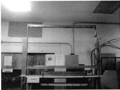
1-2 Atmospheric thinkness X at a zenith angle 0. . . . 17 2-1 The photograph of the apparatus used in this project. Two AMS

scintillator counters are mounted in the upper and lower side of the m etal fram e.. . . . .. . . . . . .. 19

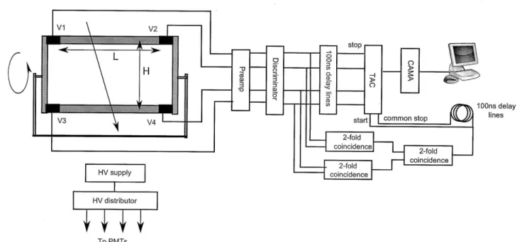
2-2 The setup of the time-of-flight method . . . . 20

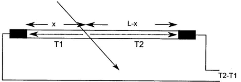
2-3 The plot shows the position the particle goes through. Photons will fly

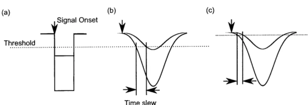
through the counter and reach both ends of counter, with flying time T 1 and T 2. . . . . 22 2-4 The plot shows the effect of time slew.(a) The ideal signal pulse with

zero falling time. (b) The signal pulses which have the same shape but with differenet amplitudes. (c) The signal pulses after amplification (notice that the scaling is different from (b).) . . . . 23

2-5 The plot shows the acceptance fo a geven zenith angle 0. . . . ... 24 2-6 The setup for the tilting method. . . . . 24 3-1 The scheme show the setup for plateauing a counter. . . . . 28 3-2 The plateau curves of all 4 channels. The arrows show where the

voltage will be set. . . . . 29

3-3 The angular distribution by tilt method. The data are collected from

three different days. . . . . 31

3-5 The differential count rate at 0 with dQ and dA . . . .. 33

3-6 The side view of the counters, showing the dimensions and the defini-tion of coordinates. . . . . 33

3-7 The telescop at 90' zenith angle. . . . . 35

4-1 The scheme of time calibration. . . . . 37

4-2 Time Calibration of Channel 0 to 3. . . . . 38

4-3 The time histograms of the two counters, with differenciated histograms. 39 4-4 The time histograms of the two counters. The peaks show a time resolution about 9 channels from an uncollimated source. . . . . 40

4-5 The setup for velocity calibration. . . . . 41

4-6 The histograms of velocity calibrations. Five peaks corresponds to x = 6cm, 36cm, 76, 111cm,131cm. Upper figure: counter VI V2. Lower figure: counter V3 V4 . . . . 42

4-7 The fitting of position of source versus time channel. . . . . 43

4-8 Ten different events, showing reconstructed path. . . . . 45

4-9 The angular distribution, without acceptance correction. . . . . 46

4-10 Acceptance versus angle. . . . . 47

4-11 The angular distribution, with acceptance correction. The data is fit with cos2_{0, with reduced chi-squared x,} = 114. . . . . 48

A-i The front panel of the LabView program. . . . . 53

A-2 The scheme of the TDC Readout Program. . . . . 54

C-1 The circuit scheme of the high voltage distributor. Only three branches out of six branches are shown for simplicity. . . . . 57

List of Tables

Chapter 1

Introduction

Cosmic rays have been a resource of energetic particles for high energy physics exper-iments. The cosmic rays are the source for the study of the high energy interaction because the energy of cosmic rays can exceed energies from particle accelerators. The study of cosmic rays has been an important and interesting subject in the field of particle physics [2]. One of the examples is that it had been used to confirm the rela-tivity effect by measuring the life time of muons in the cosmic rays. Parity violation is also observed in the muon decay. The study of the angular distribution of cosmic rays is important because it gives us a way to study the high energy interaction of muons. Since the primary cosmic rays are protons and He nuclei, the showers and cascaded interactions produce the muons (93%) we observe on earth. Exact modeling is possible from accurate measurements. We may also be able to guess what kind of interactions happened in the cosmic rays.

In this project, I will help Prof. Becker to develop an experiment to measure the angular distribution of cosmic rays. This setup will also be used in the future MIT graduate laboratory class, 8.811 or 8.812.

1.1

Cosmic Rays

The cosmic ray flux at the top of the earth atmosphere is about 1000 particles per square meter per second[3]. Those particles, called primary cosmic rays, are ionized

nuclei. About 79% of weight is protons, 15% is helium nucleons, and the rest consists of heavier nuclei, such as oxygen, carbon, and iron. The primary cosmic rays mostly come from outside the solar system but within the galaxy. The range of energies of cosmic rays is extremely wide, from a few GeV to 102 eV. The origin of cosmic rays and how they get so energetic are the fundamental questions of cosmic ray physics.

When the particles enter the solar system, the energy spectrum of those particles are modulated by the solar winds. There is a strong dependence of the intensities of cosmic rays with energy less than 5 GeV on solar activity. 11-year and 22-year intensities variations has been observed: when solar activity is higher, the cosmic ray intensity is lower, and vice versa. At the moment, May 2010, the sun activity is roughly at minimum [4]. The geomagnetic field of earth also plays an role in the modulation. Low energy cosmic rays must overcome and panetrate the magnetic field of the earth before they can reach the top of the atmosphere.

1.1.1

Cosmic Rays in the Atmosphere

After entering the atmosphere, the primary cosmic rays interact with the nuclei and molecules in the air, mostly at 15 km above the sea level. Incident hadrons collide with atmospheric nuclei, undergo strong interactions, and secondary particles are produced. Most particles produced from the hadrons collisions are pions. Energetic primary rays and heavy nuclei will continue to propagate in the atmosphere and inter-act with the atmosphere, producing more particles. At the same time, the secondary hadrons produced from the collisions will also interact with atmosphere, or undergo decay. The particles gradually transform into leptons (muons, electrons, neutrinos) and gamma rays; those particles are the main components of cosmic rays at sea level. The particles originating from a single cosmic ray are called air showers (see Figure

1.1.2

Cosmic Rays at Sea Level

Muons are the main component of cosmic rays observed at sea level. Most of the muons are produced at 15 km above sea level, from the decay of charged mesons, including pions and few kaons.

7rF ± p* 1t + vA(L7A)_{~ -+b~+v,~z2~)(1.1)}

K± -+ p± + v,(i2)(branching ratio ~~ 63.5%)

Muons have life time about 2.2ps in the rest frame [5]. However, because of the relativistic time dilation, most of the muons survive in the propagation in atmosphere and reach the ground. The average energy of muons at sea level is around 4GeV. Since the mass of a muon is about 105 MeV, the time dilation is about 40 times longer in average, which is long enough for the muons to reach the ground.

Because muons and muon neutrinos are associated via pion decay, the measure-ment of muons at the place they are produced can be used to calibrate the atmospheric muon neutrino flux. Also, muons decay into elections and neutrinos.

p--+ e- + 1e + V,

Therefore, muons play an important role in today's neutrino oscillation experi-ments.

1.2

Zenith Angular Dependence of Muon Intensity

Previous measurements have shown that the muon intensity depends on the zenith angle strongly but not on the azimuthal angle.

According to [1], the zenith angle dependence of the intensity can be expressed as Equation 1.3, assuming that the curvature of the Earth can be neglected, and that the intensity depends only on the amount of matter the particles traveled through.

I(0, Xh) = I(0 0, Xh) exp (1 - sec()) (1.3)

Therefore, the intensity depends on Xh sec(O) only. Here, Xh is the vertical depth in g/cm2

, A is attenuation length in g/cm2 _{of a particle passing through matter.}

The quantity Xh _{sec(O) is called the slant depth and can be understood from}

Figure 1-2.

Generally, the zenith angle dependence can be expressed as

I(0, Xh, E) = I(0) cosn(EXh)(0) (1.4)

where the power n depends on the energy and the atmospheric depth. The overall angular distribution of muons has n ~ 2 from experiments[5]. A summary of previous data is presented by J. Kempa and I. M. Brancus[6].

conn

Figure 1-1: The figure shows from [1]

ComKnet

the production of particle in the atmosphere. Adopted

Xh O X

Chapter 2

Experimental Setup

2.1

Apparatus

The main apparatus in this project are two AMS-01 scintillator counters, built by A. Zichichi's group in Bologna to space qualification [7]. The dimensions of the counters are 134 cm x 11 cm x 1.0 cm. The two scintillators are mounted on a metal frame, which can be rotated to point to different zenith angles. This setup can be viewed as

a muon telescope.

Figure 2-1: The photograph of the apparatus used in this project. Two AMS scintil-lator counters are mounted in the upper and lower side of the metal frame.

muons: time of flight measurement, and direct measurement. Each method will use the same apparatus, but in different configurations.

2.2

Time-of-Flight Method

The first method is the time difference and time of light methods. When muons go through the scintillator counters, photons will be produced and travel to the two ends of the scintillator counters. The photons will be collected and transformed into electrons by photoelectric effect. Then the electrons are amplified by the PMTs, producing a electric signal output, with negative polarity. With the time difference between the two signals from the ends, we can calculate where the muons go though the counters.

To PMTs

Figure 2-2: The setup of the time-of-flight method

2.2.1

Signal Chain

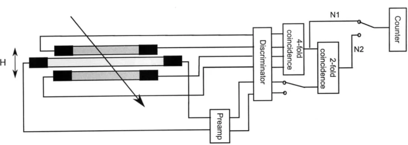
The complete setup of instruments of this method is shown in Figure 2-2.

After the photons are collected and amplified by the PMTs, the output electric signals are fed into a preamp (LeCroy 612A) in order to reduce the time slew effect,

1OOns delay lines

which will be explained below. The outputs of the preamps are then fed into discrim-inator (LeCroy 623Z) channels to produce digitized outputs. The triggering level of the discriminator is set to be -20 mV, which means when the input signal pulse is less then -20mV, a digital one signal will show up at the output. The digital pulse is

-600 mV high and 100 ns wide.

The outputs of the discriminator are then fed into a coincidence unit(LeCroy 465) (See the figure for the connections). The coincidence will output logic one when the input signals are both logic one and overlap in the time domain. There are two main functionalities of the coincidence. First, the coincidence is used to distinguish signal from noise. In order to operate the PMTs in the high detection efficiency region, the supply voltage of the PMTs must be made high enough. However, noise will also be amplified significantly, and thus the counts caused by noise will be more than by particles. One way to separate signals from noise is by coincidence. The photons caused by particles will travel to the both ends of the counters, and the signals will show up in both ends with time difference less than L/v. Therefore, if a signal pulse is detected at one end of the counter, and no signal pulse is detected in the other end after L/v, then the detected signal must be noise. Secondly, the coincidence is used to select the events we are interested in. In this project, only particles that go through both counters are under consideration. Thus the output of the coincidence is used to gate the subsequent instruments in the signal chain.

The output of the coincidence is then fed into the start channel of TDC (LeCroy

2228A). The individual outputs of discriminator are connected to 100 ns delay lines,

and then connected to each of the stop channel of the TDC. The TDC will digitize the time difference between start and stop signals. The result will be read out by a LabView program via CAMAC controller. The nominal resolution of the TDC is 250ps, or of the order of 1 x 108m/s x 250ps 2.5cm. However, the exact time resolution must be calibrated.

Determine the Position

I__T2-T1

Figure 2-3: The plot shows the position the particle goes through. Photons will fly through the counter and reach both ends of counter, with flying time Ti and T2.

From the plot we have that

T1 = - (2.1) V T2= L-x (2.2) V Then V L z = -(T1 - T2) + - _(2.3) 2 v

However, the light velocity in the scintillator counter is an unknown parameter and must be measured. One way to measure the light velocity is by putting a particle source at some places on the counter and measure the time differences TI -T2. Then, the velocity can be obtained by finding out the slope of x versus TI - T2.

Time Slew

In the time of flight method, one important effect to be considered is the time slew. Ideally, if the output PMT signal has a sharp edge, or zero falling time, then the time interval between the input and the output of the discriminator should be constant (the propagation delay of the discriminator).

However, in reality, the falling time of the pulse is not zero, and the slope (dv/dt) depends on the pulse height of the input signal. In this case, the time interval will also depend on the pulse height of the input signal. This effect is called time slew. Time slew is unwanted, because it affects the position measurement.

The way to minimize the time slew is by amplifying the signals of PMTs before fed into the discriminator. Being amplified, the signals will have a steeper falling

(a) (b) (c) Signal Onset

Threshold ... ... .. ...

Time slew

Figure 2-4: The plot shows the effect of time slew. (a) The ideal signal pulse with zero falling time. (b) The signal pulses which have the same shape but with differenet am-plitudes. (c) The signal pulses after amplification (notice that the scaling is different from (b).)

edge, and therefore the effect of time slew will become smaller. In our experiment, the signal is connected into a preamp, which has gain of about 10 V/V. Therefore, the time slew is approximately 10 times less than before.

2.2.2

Solid Angle Acceptance Calculation

Once the positions where the particles go through are found, the zenith angle of the path can be calculated. If a muon pass through the upper counter at z" and the lower

counter at x1, then the zenith angle will be 6 = tan-'(XUHX).

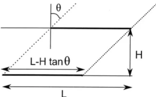
However, there is one more correction to be made before the angular distribution can be obtained - the acceptance ratio of the telescope. Muons with incoming zenith angle 0 will be considered for the following discussion (see Figure 2-5). From the figure, it is clear that not all the mouns hitting the upper counter will also hit the lower counter. Only those muons in the bold region in the figure will pass both

counters. The portion of muons to pass both counters depends on the zenith angle. Thus, different zenith angles have different acceptance ratios, which we must take into account in order to get the correct angular distribution.

0.~

L-Htan0 .. H

Figure 2-5: The plot shows the acceptance fo a geven zenith angle 0.

V1 v3 0

Figure 2-6: The setup for the tilting method.

2.3

Tilting Method

The second method is to tilt the setup to measure the count rate at different zenith angles directly. We can tilt the two counters so that they point to the zenith angle we want to measure, see Figure 2-6.

2.3.1

Detection Efficiency

The particle detection efficiency mainly depends on the voltage of the PMTs. When the voltage is low, the gain of the PMT is too low to overcome the threshold of the discriminators, and thus the detection efficiency is low. The gain and the detection efficiency increase as the voltage increasses. At some point, the detection efficiency will reach the highest value. A good counter should provide over 99% detection efficiency. The detection efficiency remains relatively constant over a wide range of supplied voltage, called the " plateau." If the voltage is further increased , noise

begins to overwhelm the signals. Therefore, the supplied voltage to the PMTs must be determined before any measurement is made.

Chapter 3

Experimental Result 1

3.1

Plateau the Scintillator Counters

The setup for plateauing the counter is shown in Figure 3-1. Two counters with a size smaller than the counter under test are placed on the top and the bottom of the test counter. The outputs of top and bottom counters are connected to the discriminator to digitize the output, and to the 4-fold coincidence. The output, called NI in the figure, is connected to a scaler. The output of the test counter is connected to the discriminator, combined with N1, to a 2-fold coincidence. This output is called N2. Notice that we will test one PMT at a time.

When there is a particle passing through the top and the bottom counters, N1 will goes to logic one. More importantly, since the sizes of top and the bottom counter are smaller then the testing counter, the particle must also pass the testing counters. Therefore, the efficiency of the counter can be measured by the ratio of counting rates of NI and N2.

N2

N7 2 (3.1)

N1

The small counters need not to be very efficient in this method, since it is the ratio that is important.

3.1.1

Plateauing Result

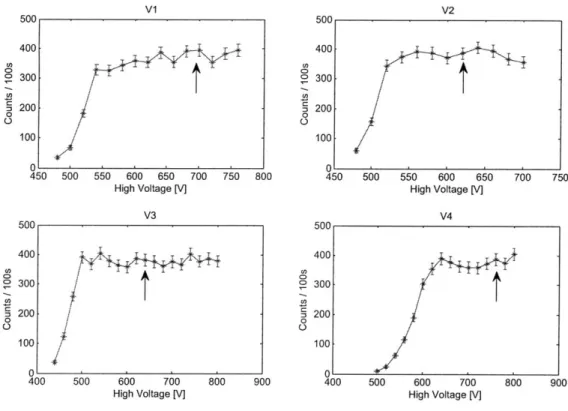
The results of plateauing are shown in Figure 3-2. The plots give the counts of N2 per 100s. N1 is the same for all four measurements. The plots show that the counts increase very fast as voltage increases, and then after a "knee", the counts enter the plateau region. The voltage of PMTs must be set in this plateau region. However, setting the voltage too high will cause lots of noise. The rule of thumb is to set the voltage 100V higher then the knee. The supplied voltages of PMTs are marked in the figure by arrows.

N10 0 00 0 ~ 8L N2 CD CL H 33

Figure 3-1: The scheme show the setup for plateauing a counter.

3.2

Tilted Counter Method

The size of counters is L = 134 i 1 cm and W = 11.0 ± 0.5 cm. The seperation

between two counters is 98 ± 1 cm.

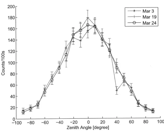
The setup is shown in figure 2-2. However, the output of the coincidence is now connected to a scaler instead of a TDC. The counters are rotated to point at different zenith angles, 9, and counts are accumulated for l00s. The measurements are done on three different days in order to check the consistency of data.

The results are listed in Table 3.1, and plotted in Figure 3-3. The data show that the counts are very consistent at different times. However, there is one outlier at 400, which deviates from the curve by more then 5 times of uncertainty. This point will be discarded for later analysis.

500 550 600 650 High Voltage [V] 600 700 High Voltage [V] 800 450 500 550 600 650 High Voltage [V] 800 900 600 700 High Voltage [V]

Figure 3-2: The plateau curves of all 4 channels. The arrows show where the voltage will be set.

The averaged data are plotted in the Figure 3-4. The data are fitted with

A cos2_{(0 + #) + C}

(3.2)

The fit results are

A = 145 ± 2 counts/100s

4

C = 11.4 ± 0.8 counts/100s with a reduced chi square of:

x = 0.91 _(3.3)

/

1

Day 1 (Counts/100s) Day 2 (Counts/100s) ' Day 3 (Counts/100s) -90 15 12 -80 20 - 17 -70 23 - 26 -60 52 - 47 -50 74 - 69 -40 92 - 89 -30 126 101 113 -20 143 148 149 -10 138 158 156 0 155 178 165 10 164 165 162 20 139 146 140 30 130 118 121 40 49* 95 89 50 65 67 71 60 54 54 47 70 25 26 26 80 19 15 18 90 13 12 12

Table 3.1: The data of the tilting method.

3.2.1

Analysis of the Data

3.2.2

The Counting Rate at 0 = 0

Consider a small portion of the telecope with area dA, pointing to the zenith angle

0, with solid angle dQ (see Figure 3-5).

Then the differential counting rate across dA and dQ, obeying the cos2 ₀

distribu-tion, is '

dN N

dt 1o Cos20(cos OdA)dQ, (3.4)

where jo is the differential flux at 0 = 0.

The side view of the counter is shown in Figure 3-6. In this project, the telescope has a long length and a narrow width, and therefore we can approximante dQ as

W cos Odx

(x - x')2 + H

2 _(3.5)

* Mar 3

- Mar 19

0E Mar 24

-40 -20 0 20 40 60 80 100

Zenith Angle [degree]

Figure 3-3: The angular distribution by tilt method. three different days.

Then the total count rate of the telescope is

dN= I f Cos2(cos OWdx')

dt 0 f

The data are collected from

(W

cos

Odx

Instead of finding the analytic solution, the integration is done numerically. The result is

d N

dt = 136.2(cm2 - sr)Io

A more accurate calculation, using the equations in [8], gives

dN

- = 135.5(cm2 _.sr)Io

which is very close to the approximate value.

(3.7) (3.8) 200- 180- 160- 140- 120- 100- 80- 60- 40- 20-0L -100 -80 -60

-80 -60 -40 -20 0 20 40 60 80 Zenith Angle [degree]

Figure 3-4: The averaged angular distribution.

Now, from

A =

Io = (1.1 ± 0.2) x 10- 2/cm 2-sr-s _(3.9)

This value agrees with previous data in [2].

3.2.3 The Counting Rate at

0

When the telescope points at 0 = 900, the counting rate should be zero if the cos2 ₀

distribution holds. However, the measured value is about 11.4 ± 0.8 per 100s. A few effects must be taken into account.

0=0

dn

dA

Figure 3-5: The differential count rate at 0 with dQ and dA

L=134cm--..

H=9cm

dA:

X'

Figure 3-6: The side view of the counters, showing the dimensions and the definition of coordinates.

Accidental Rate

The first correction need to be done is the accidental rate. Eventhough the coincidence method is used to reduce the noise, it is still possible that the noise show up at both ends of counter at the same time. The rate of such accident event, called accidental rate, are given by

Racc= 2TN1N2, (3.10)

where -F is the pulse width of the output of each discriminator module, and N₁ and N2 are the raw count rates of upper and lower counters, respectively.

In our setup, we have r = 100ns, Ni = N2 = 5000/100s. Therefore,

Racc= 5/100s (3.11)

Finite Acceptance

When 0 = 90', the width of the counters now plays an important role and cannot be ignored. From Figure 3-7, we have 0' = 90 - 0. Since the width is small comparing

to the seperation H between the counters, we have 0'

<<

Therefore, the counting rate is

dN = 1f

jo

0'Ldx') (L c2s dx _(3.12)

Plugging the values into the equation, we get

dN2

dt = 3.7(cm2 .sr)Io (3.13)

With Io = (1.1 ± 0.2) x 10- 2_/cm 2_{-sr-s, we can find that the counts per}

100s are 4.0 ± 0.7 for this correction.

Therefore, the sum of the count rates from these two effects are 9 ± 1 per 100s, which is still less than the measured count rate. The last effect that will contribute to the count rate at zero zenith angle is the air shower. From our measurement, the

... . . ... ... .W =1 cm

H=134cm >.

Figure 3-7: The telescop at 900 zenith angle.

remaining counting rate for air showers would be

Rairshower = 2 ± 1/lOs, (3.14)

Chapter 4

Experimental Result 2

4.0.4

TDC Time Calibration

In the time of flight method, the positions of the muons are determined by the time difference. Therefore, the TDC must be calibrated to achieve higher accuracy. The calibration setup is shown in Figure 4-1. A pulse source is fed into the START of the TDC and a delay box, which allows to change the delay time from 0 to 31 ns. The delayed signals are fed into the STOP channels of the TDC. When the pulses show up at each of the STOP channels, the TDC will stop the conversion. Then the calibration curve of individual channels is obtained by fitting the results into linear functions, as shown in Figure 4-2.

source stop

70-- 70 0.246*x+13.385 [ns] 0.251*x+13.625 [ns] 60- 60 . 50 50 040 40-- - Channel 0 30 Channel 1 Best Fit

30Best Fit Best Fit

60 80 100 120 40 160 180 200 220 60 80 100 120 140 160 180 200 220 channel(x) channel(x) channel2 channel3 70 70 0.250*x+13.827 [ns] 0.247*x+14.205 [ns] 60. 60-£50 £50 40 - 40-30 - - Channel 2 30 Channel3

Best Fit Best Fit

60 80 100 120 140 160 180 200 220 60 80 100 120 140 160 180 200 220

channel(x) channel(x)

Figure 4-2: Time Calibration of Channel 0 to 3.

4.1

Resolution of Counters

The time resolution of the TDC is set to be 250ps per channel, and the nominal refraction index of scintillator is n ~ 1.59. Therefore, the TDC resolution contributes an uncertainty of Ax = !At = 2.4cm. However, the resolution is also limited by the time resolution of counters. We used two methods to measure the resolution of counters.

Differentiation Method

In this method, we let the counts accumulate to obtain time histograms of two coun-ters(see Figure 4-3). Ideally, the histogram will have a rectangular shape. However, due to the limited resolution of the counters, the edge of the histograms are gradu-ally rounded of. If we differentiate the falling edge of histograms, we can obtain the resolution of the counters.

channel 1

2000 1500 1000 500 0 1I -Y IY v yyy y yv -- ,- __ -25 -20 -15 -10 -5 0 5 10 15 20 25 Time Difference [ns] 01 ---- I 'V V'1'I \J\4 '-JJV i I -25 -20 -15 -10 -5 0 5 10 15 20 25 Time Difference [ns]

2060 2080 2100 Channel 2120 2140 2160 Ch34 2060 2080 2100 2120 2140 2160 Channel

Figure 4-4: The time histograms of the two counters. The peaks show a time resolu-tion about 9 channels from an uncollimated source.

From Figure 4-3, we obtain that the time resolution is about 1 ns, which corre-sponds to 9 cm.

Particle Source Method

Another way to measure the resolution is directly put an particle source on the counter and let the histogram accumulate. The histograms are shown in Figure 4-4, with the source putting in the middle of the counters. The peaks have FWHM about 9 chan-nels, or 2.25ns, or 21cm. Then, assuming Gaussian distribution, o = FWHM/2.35 =

9cm Ch12 ^' A^,- 0-2040 100r- 60-2040

24ns delay lines

Figure 4-5: The setup for velocity calibration.

4.2

Velocity Calibration

In order to convert the channels to positions, we must calibrate the velocity of the counter. The way we do this is almost the same as the measurement of resolution, but now we put the source on several places on the counter, and take measurements. Figure 4-5 shows five of the measurements. After the histogram is obtained, the mean value and the standard deviation of each peak are calculated. Then the position versus the average channel is plotted and fit to linear equations.

The fit results are

os = (1.67 ± 0.01) x channel - 100[cm] _(4.1)

x, = (1.48 ± 0.01) x channel - 68[cm]

Notice from Figure 4-7 that the velocity slightly changed close the edge of counter. However, since the change is much less then the resolution of the counters, the effect can be neglected.

4.3

Time-of-Flight Method

With the relations between the time, the channel, and the position, now we can reconstruct the path of muons. The two counters are moved closer, with seperation of H = 7.6 ± 0.2cm between the counters. The histogram is accumulated for roughly

100000 events. Then the paths are reconstructed by the relations we have. Ten events

50 40-z 30-0 20- 10-0 &L 2000 2020 2040 2060 2080 2100 2120 2140 2160 2180 220 Channel 60- 50- 40-U, 5 30-0 20- 10-0 - '''-^^ '"^^-2000 2020 2040 2060 2080 2100 2120 2140 2160 2180 220( Channel

Figure 4-6: The histograms of velocity calibrations. Five peaks corresponds to x =

6cm, 36cm, 76, 111cm,131cm. Upper figure: counter VI V2. Lower figure: counter V3 V4

0

---- V1V2 110- _BestFit -90-E 2 70-0 o 50- 30- 10--10 40 60 80 100 120 140 Channel 130-110. V3V4 110 -BestFit 90-E 1= 70. o 50-a. 30 10 -10 40 60 80 100 120 140 Channel

0 = tan- ( H i) _(4.2)

where x, is measured from VI, and x, is measure from V3. The raw angular distribution histogram is shown is Figure 4-9.

Now we have to correct for the acceptance ratio at different zenith angles. The acceptance ratio is done by the Monte Carlo method (See Appendix B.) The accep-tance ratio is plotted in Figure 4-10, and the corrected histogram is shown in Figure 4-11. A cosine square function is also plotted. The result again agrees with the cosine square distribution up to 70'. Notice how the acceptance correction affect the count rates at large angles, resulting in a tail, which agrees with the result of method 1.

, 5 . E 0 - - - -. .-.. ..-.. .-.. -5 0 50 [cm] 10-5 E . 0 -. . - -I - -- -- - - -10 5 100 150 10 0 50 [cm] 100 150 0 50 100 1 [cm] 10 5 0--5 0 50 100 1E [cm] [cm] 10 5 E -0 -5 [cm] 100 150

Figure 4-8: Ten different events, showing reconstructed path.

[cm] [cm] [cm] [cm] -.. . . . . . . . .-. -. . , , 5 E . .. . .

12000 10000- 8000- 6000- 4000- 2000-0 -80 -60 -40 -20 0 20 40 60 80 Theta(degree)

0 0.6-0 E 0.5-Cu 0. 0 0.4- 0.3- 0.2-0.1 -0 -100 -80 -60 -40 -20 0 20 40 60 80 100 Theta (degree)

12000 10000 8000 6000 4000 2000 0

Figure 4-11: The angular distribution, with acceptance correction. with cos2o, with reduced chi-squared Xu = 114.

The data is fit

-80 -60 -40 -20 0 20 40 60 80 Theta(theta)

Chapter 5

Conclusion

To examine the angular distribution of cosmic ray muons, we setup a muon tele-scope to measure the zenith angular distribution. The telecsope consists of two long scintillator counters with double-ended readout, which enable the use of time of flight method. It has been well known that the intensity of muons obey a cos2 0 dependence with tails on the horizontal. We used two different methods to measure the zenith angle dependence. The first method is by rotating the whole setup to point at the zenith angle under measurement. Second method is by time of flight measurement. With the double-ended readout, the position where a muon passes through can be reconstructed from the time difference between the signals at the two end. Both mea-surements confirmed the cos2 0 distribution, with a 'tail' at large zenith angle, which

Appendix A

2228A TDC Readout Program

This Labview program is used to read out the data from a 2228A TDC module in a

CAMAC crate. The program will read the data after the digitization completes, clear

the data registers in the TDC, and then ready for the next readout. The program will run and extract the data continuously, and the data is displayed in a histogram. The user can choose which channel to be displayed by changing the field "display channel." The elapsed time will also be displayed on the panel. Once the STOP button is pressed, the program will stop reading the data from TDC, and will ask the user to save the data. The file paths can be specified in the data path fields. Three files will be saved. First one, channel data, will contain all the raw data from all 8 channels. Channel data has eight columns, representing 8 channels of the TDC. Another one, histogram, will contain the histograms of all 8 channels. The last one the the difference histogram, which will contain the histogram of the difference of the two selected channels. The data files will be text files, which can be imported into matlab for further analysis. Histogram files will have 8 rows, representing 8 channels of the TDC. Notice that the program will read all eight channels of the TDC, whether the channel is connected or not.

There are a few input parameters of this program.

* VISA session : The GPIB address of the instrument, or CAMAC crater

o Module Address: The address of TDC module in the crater.

Four of the parameters are used to control the histogram: number of bins, max, min, inclusion.

" Number of bins: how many numbers of bins in the histogram " Max, min : the range of histogram

" Inclusion: Whether the bins should include the upper or lower boundary Notice that after the program starts, changing of these parameters will have no effect.

Figure A-1: The front panel of the LabView program.

53

]N

cg

05IW t Dfeec hne ru ifference Chaninel D i e-ceChnn Timer ms)23456 79 etnum be %2 CeDta Path 24 bIs b oaule Address ineTriansfer A CRSA R eo ] Deaser ihbit 2 CDI (D Cdl- C:l (D CD C) CD

-h-7.1l11

2

Appendix B

Monte Carlo Simulation of

Acceptance Ratio

theta = (2*rand -1)*pi; dx = sin(theta); dz = -cos(theta); x_0 = x - Lz * dx / dz; if x_0>0 & x_0 < L-x; hit = hit + 1; hittheta(hit) = atan( end (x_0-x)/L-z); end

numberof-bins = 50;

thetabins = -pi/2 :pi/number-ofbins:pi/2;

[N-theta,X_theta] = hist(hit_theta(1:hit) ,theta-bins);

figure;

Appendix C

High Voltage Distributor

An high voltage distributor is made for this project. The distributor is used to supply up to six photomultiplier tubes with sigle voltage supply module.

Figure C-1: The circuit scheme of the high voltage distributor. Only three branches out of six branches are shown for simplicity.

Bibliography

[1] Peter K.F. Grieder. Comsic Rays at Earth: Researcher's Reference Manual and

Data Book. Elsevier, 2001.

[2] B. Rossi. Interpretation of cosmic-ray phenomena. Review of Modern Physics,

20(3), 1984.

[3] Thomas K. Gaisser. Cosmic Rays and Particle Physics. Cambridge University

Press, 1990.

[4] National Oceanic and Atmospheric Administration. Solar cycle progression and prediction. http: //www. swpc .noaa. gov/SolarCycle/.

[5] C. Amsler et al. (Particle Data Group). The review of particle physics. Physics

Letters, B667(1), 2008.

[6] J. Kempa and I. M. Brancus. Zenith angle distributions of cosmic ray muons.

Nuclear Physics B (Proc. Suppl.), 112, 2003.

[7] M. Aguilar et al. The alpha magnetic spectrometer (ams) on the international space station: Part i v results from the test flight on the space shuttle. Physics Reports, 366, 2002.

[8] R. P. Kane and U. R. Rao. Zenith angle response of a vertical meson telescope.