HAL Id: insu-02377739
https://hal-insu.archives-ouvertes.fr/insu-02377739
Submitted on 24 Nov 2019
HAL is a multi-disciplinary open access
archive for the deposit and dissemination of
sci-entific research documents, whether they are
pub-lished or not. The documents may come from
teaching and research institutions in France or
abroad, or from public or private research centers.
L’archive ouverte pluridisciplinaire HAL, est
destinée au dépôt et à la diffusion de documents
scientifiques de niveau recherche, publiés ou non,
émanant des établissements d’enseignement et de
recherche français ou étrangers, des laboratoires
publics ou privés.
Sedimentation instabilities: Impact of the fluid
compressibility and viscosity
Michael Niebling, Eirik Flekkøy, Knut Jørgen Måløy, Renaud Toussaint
To cite this version:
Michael Niebling, Eirik Flekkøy, Knut Jørgen Måløy, Renaud Toussaint. Sedimentation instabilities:
Impact of the fluid compressibility and viscosity. Physical Review E : Statistical, Nonlinear, and
Soft Matter Physics, American Physical Society, 2010, 82 (5), �10.1103/PhysRevE.82.051302�.
�insu-02377739�
Sedimentation instabilities: Impact of the fluid compressibility and viscosity
Michael J. Niebling,1 Eirik G. Flekkøy,1Knut Jørgen Måløy,1 and Renaud Toussaint21
Department of Physics, University of Oslo, P.O. Box 1048, 0316 Oslo, Norway
2
Institut de Physique du Globe de Strasbourg, CNRS, and University of Strasbourg(EOST), 5 rue Descartes, 67084 Strasbourg Cedex, France
共Received 18 May 2010; published 11 November 2010兲
The effect of an interstitial fluid on the mixing of sedimenting grains is studied numerically in a closed rectangular Hele-Shaw cell. We investigate the impact of the fluid compressibility and fluid viscosity on the dynamics and structures of the granular Rayleigh-Taylor instability. First we discuss the effect of the fluid compressibility on the initial fluid pressure evolution and on the dynamics of the particles. Here, the emerging patterns do not seem highly affected by the compressibility change studied. To characterize the patterns and motion the combined length of the particle trajectories in relation to the movement of the center of mass is analyzed, and the separation of particle pairs is measured as a function of the fluid viscosity.
DOI:10.1103/PhysRevE.82.051302 PACS number共s兲: 45.70.⫺n, 45.50.⫺j, 47.11.⫺j
I. INTRODUCTION
Granular materials play an important role in geological processes, for example, in erosion or avalanche processes 关1–3兴. Handling granular materials is in addition the daily
basis of many of our industries, such as mining, agriculture, civil engineering, and pharmaceutical manufacturing. The field of dry granular materials and the enormous richness and complexity of granular motion and granular flows have pro-vided the research of the last 20 years with numerous ques-tions. In granular flows the presence of an interstitial fluid has been shown to strongly affect the dynamics of the grains 关4–8兴. The fluid compressibility and the fluid viscosity may
well have an effect on the dynamics of the grains, for ex-ample, in fluidized bed reactors, but have not been in much focus.
The Rayleigh-Taylor instability in granular fluid mixtures has been studied with different types of fluids. With air the influence of the grain size was systematically investigated 关9–11兴, and the behavior of this instability was compared
between the cases where the interstitial fluid was air or water-glycerol 关12兴. In a comparable study of the
Saffman-Taylor instabilities for granular-fluid mixtures oil or air was utilized as the interstitial fluid关13,14兴. In our previous work
关12兴 we have found in experiments and simulations that the
mixing of the grains with the fluid during the granular Rayleigh-Taylor instability was very different whether we used air or a water-glycerol solution as the interstitial fluid. In pursuit to study this influence we further developed a numerical model关9,10,13,15兴 that was proven 关12兴 to
repro-duce well the experimentally measured dynamics of the grains in the presence of a fluid. Even though we could give a quantitative explanation with the characterization of the correlation lengths and velocity field histograms, it is still an open question if the mixing behavior is a result of the fluid grain coupling to a compressible or incompressible fluid and how big is the influence of the fluid viscosity. To further answer this question we will perform numerical simulations with the goal to study the effect of the fluid viscosity and fluid compressibility on the mixing behavior during sedimen-tation. For this purpose the fluid viscosity and fluid
com-pressibility are systematically and independently varied. These simulations show that the fluid compressibility has a small effect on the mixing except in extreme cases. The change in the fluid viscosity leads to an increase in the av-eraged particle trajectory length as a function of the displace-ment of the center of mass of the particles. With respect to the separation of particle pairs, the change in the viscosity displays initially two regimes: a nonhydrodynamic or ballis-tic regime at low fluid viscosities and a hydrodynamic re-gime at high fluid viscosities, with a crossover from diffusive to turbulent-dispersive behavior. This distinction however does not hold for the later stages of the simulations.
The paper is organized as follows. In the next section the implementation of the numerical model is briefly discussed. For more details and explanations see 关9,10,12,13,15兴. The
results of the simulations with varied fluid compressibility and viscosity are presented in Sec. III. In Secs. III A and
III B the effect of the fluid compressibility is studied. The effect of the fluid viscosity is studied and discussed in Sec.
III Cfollowed by the conclusions in Sec.IV.
II. THEORY AND SIMULATIONS
The numerical model is a two-dimensional hybrid model that uses a continuum description for the fluid and a discrete description of the granular phase. Friction between particles or the particles and the side plates is neglected. Further we neglect the friction between the fluid and the side plates. The model is derived in detail in 关9,10,12,13,15兴. It was tested
and shown to reproduce the dynamics of granular flows at low Reynolds numbers, and we will only present the main equations for the evolution of the nonhydrostatic part of the pressure field P and the dynamics of the particles briefly.
A. Dynamics of the fluid
The equations ruling the evolution of the nonhydrostatic part of the pressure, also termed the hydraulic head P, are derived in detail in Ref. 关15兴. The nonhydrostatic part of the
pressure, P, corresponds to P = P
⬘
−fgy⬘
, where P⬘
is the pressure, g is the gravity constant,fis the fluid density, andy
⬘
is the depth. In the following we will only present and discuss the main equations briefly. We start with mass con-servation of the fluid:t关f共P兲兴 + ⵜ · 关f共P兲vf兴 = 0, 共1兲
where vfis the velocity of the fluid andis the local
poros-ity: for the mass conservation of the grains we get
t共1 −兲 + ⵜ · 关共1 −兲u兴 = 0, 共2兲 where u is the velocity of the grains. The velocity vf of the
fluid is the sum of the local velocity relative to the grains, derived from Darcy’s law, plus the velocity of the grains:
vf= u −
ⵜ P, 共3兲
whereis the fluid viscosity andis the local permeability. Using Eq.共3兲 in Eq. 共1兲 we get:
t关f共P兲兴 + ⵜ ·
冋
f共P兲冉
u −
ⵜ P
冊
册
= 0. 共4兲Eliminatingtbetween Eqs.共2兲 and 共4兲 and taking the fluid mass densityf共P兲 to be related to the pressure by the com-pressibility T= −共1/V兲V/P through an equation of state that we linearize around the background pressure P0with0f as the fluid mass density at P0,
f共P兲 ⬇Tf
0共P − P 0兲 +f
0
, 共5兲
we get after a short calculation a diffusion equation for the nonhydrostatic part of the pressure P. This equation in gen-eral implies the fluid compressibility 关15,16兴:
冋
Pt + u ·ⵜP
册
=ⵜ ·冋
Pˆ 共T兲
ⵜ P
册
− Pˆ 共T兲 ⵜ · u, 共6兲 where we have defined Pˆ 共T兲=f/共f0
T兲= P− P0+ 1/T. Since in this work we only simulate fluids with the mass density of air as the interstitial fluid, we can neglect the inertia and the weight of the fluid, and the hydraulic head correspond to the local pressure: P
⬘
⬇ P. In the case of air, considered as an ideal gas we getT= 1/ P0at P0and Eq.共6兲results in
冋
Pt + u ·ⵜP
册
=ⵜ ·冉
P
ⵜ P
冊
− Pⵜ · u. 共7兲At the other end of fluid compressibility types, the incom-pressible limit where T→0, Eq. 共6兲 results in a Poisson equation:
ⵜ ·
冉
ⵜ P
冊
=ⵜ · u. 共8兲In both cases we calculate the local permeability by the Carman-Kozeny relation关17兴 = a 2 9K 共1 −s兲3 s2 , 共9兲
wheres= 1 −is the solid volume fraction, a is the particle radius, and K = 5 is an empirical constant valid for a packing of beads关15兴.
B. Dynamics of the particles
The force equation for a single particle with the velocity
vp, particle mass m =ma2h, particle mass densitym, vol-ume Va=a2h in a cell with a plate spacing of h, and the number density defined as n=sm/m is given by
mdvp
dt =effVag + FI−
ⵜP
n
+ Fd, 共10兲
whereeff=m−f enters in the buoyancy forces in the first term of the left-hand side, FIis the interparticle solid contact
force, the third term arises from the momentum exchange between the fluid and solid, and Fd is a viscous force
ac-counting for energy dissipation. To approximate a situation of hard spheres we choose the interparticle force FI be a
linear force with a spring constant k high enough to make the overlap of particles during collision a negligible fraction of their diameters.
If particles collide we include energy dissipation with a restitution coefficient of rs= 0.13关10兴. This is modeled by a viscous force, active only during particle contact. This force is proportional to the relative velocity of the particles vrand
oriented along the unit vector nd, which points from the
cen-ter of one particle to the contact point:
Fd= −␥d共vr· nd兲nd. 共11兲
The particle propagation is modeled by the velocity Verlet scheme关18,19兴.
III. RESULTS
For the simulations presented in this paper we used a Hele-Shaw cell in the x direction of⌬x=5 cm in width and in the y direction ⌬y=7 cm in height. The cell is entirely closed on all sides, both for the fluid and for the grains. The mass density of the fluid was constant, set to the mass den-sity of airf= 1.29 kg/m3, and we considered particles of a mass density of m= 2500 kg/m3. The initial pressure con-sidered corresponds to atmospheric pressure, P0= 100 kPa at
the top of the cell. The average size of the particles is 140 m and to avoid the formation of a triangular lattice the particle diameter was defined to have a flat size distribution with a range of ⫾10% variation about the mean. In total approximately 140 000 particles are considered in the simu-lations. The only variables that we vary in the following are the viscosity of the fluid f and the compressibility of the fluid T. The initial state is prepared in the following way: particles are first let to rest on the bottom up to when a fraction of 2/3 of the cell volume is filled. The interparticle space is filled with the interstitial fluid considered. Then, gravity is instantaneously reverted, corresponding to a sud-den upside down flipping of the cell, and particles start to fall
NIEBLING et al. PHYSICAL REVIEW E 82, 051302共2010兲
from their initial configuration and initial zero velocity. In all the simulations the cell could be divided into three zones independent of the type of fluid. In the base of the cell, where particles have sedimented, and in the top section we find a bulk of compacted particles. In these two sections particles are hardly moving relative to each other. In between these two sections, we find a dynamic section with mobile dispersed particles. The particles in this section move while forming fingers of higher particle density and bubbles of lower particle density.
A. Effect of the compressibility on the granular Rayleigh-Taylor instability
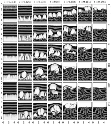
The dynamics of the particles in the Hele-Shaw cell sig-nificantly depends on the interstitial fluid. In vacuum we do not see any evolution of patterns in the density field as shown in Fig. 1. Since all particles start at zero velocity, indeed, they simply all homogeneously fall in free fall, up to the moment when they contact the lower boundary and bounce back. In Fig.2an interstitial fluid however is present. While falling through the gap of fluid, here the particles de-velop downward falling fingers of high particle density and rising bubbles of low particle density. In this section we are going to investigate the effect of the fluid compressibility on the dynamics of the particles. In Fig.2we therefore vary and compare the dynamics for different fluid compressibilities. While the fluid viscosity is kept fixed and set to f共air兲 = 0.018 mPa s, which corresponds to air at room conditions of 25 ° C and atmospheric pressure, the bulk modulus varied fromT= 1/T= 1 kPa to incompressible behavior.
From the plots of the density field in Fig.2 we can iden-tify two main differences due to the change in compressibil-ity. First we find for the high compressible cases with a bulk modulus of Tⱕ5 kPa that at times tⱕ0.12 s bubbles of low particle density appear at the upper end of top section and right above the fingers in Fig. 2 in the picture at t = 0.126 s in the top row. For a higher bulk modulus these bubbles are not present, and the top section stays uniformly compacted. Second we notice that in the beginning the center of mass of the whole top section moves further down the more compressible is the fluid. This movement of the top section stops when the weight of the packing is balanced by the overpressure of the compressed air in the base and the underpressure in the upper part of the cell. In Fig. 3 we
plotted the movement of the center of mass of all particles ⌬Rc共t兲=Rc共t兲−Rc共0兲 in time. In the plots we observe oscil-lations of the top section for all the bulk moduli below T ⱕ5 kPa. Above this limiting bulk modulus, the movement of the center of mass does not seem to be influenced by the compressibility of the fluid. The oscillations are governed by the inertia of the mass of the grains in the top section and the elasticity of the fluid given by the bulk modulus. After the pressure rises in the bottom part of the cell fluid seeps through the porous media, exchanging momentum between the particles and the fluid and damping the oscillations. The system can show transient oscillations, which we observe for
Tⱕ5 kPa or be in an overdamped regime for T⬎5 kPa. t =0s 0 2 4 0 2 4 6 t =0.018s 0 2 4 t =0.036s 0 2 4 t =0.054s 0 2 4 t =0.072s No A ir 0 2 4
FIG. 1. A layer of beads falls through a gap in vacuum. Time progresses from left to right. White areas represent areas where the particle density is zero. The gray and black areas represent areas filled with particles, and the stripes are added artificially to better demonstrate the dynamics. From left to right time progresses in equal time steps.
t =0.054s 0 2 4 6 t =0.126s t =0.198s t =0.27s t =0.342s t =0.414s t =0.486s κ T (k P a) = 1 0 2 4 6 2 0 2 4 6 5 0 2 4 6 100 0 2 4 6 2000 0 2 4 0 2 4 6 0 2 4 0 2 4 0 2 4 0 2 4 0 2 4 In f 0 2 4
FIG. 2. Comparison of simulations with different fluid com-pressibilities at a fluid viscosity of air:f共air兲=0.0182 mPa s. Gray and black areas represent areas filled with particles. The stripes are added artificially to better demonstrate the dynamics. From left to right time progresses in equal time steps and from top to bottom the bulk modulus is increased.
FIG. 3.共Color online兲 The y position of the center of mass of all particles is plotted in time for different bulk moduli.
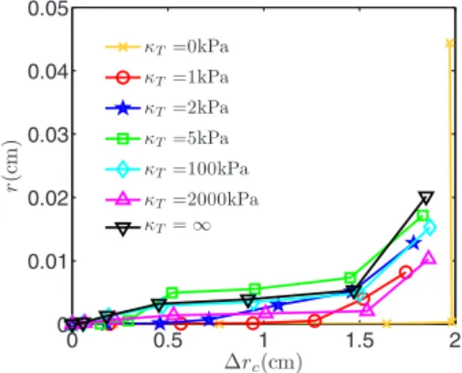
In Fig. 4 we analyzed the excess path length r共t兲 of the lowest layer of N = 8000 particles at t = 0 s, where the posi-tion of the ith particle is given by ri共t兲. The displacement of the center of mass of the lowest layer of N = 8000 particles is ⌬rc共t兲=rc共t兲−rc共0兲, and we define the excess path length r共t兲 as r共ts兲 =
兺
Ni兺
j=1 s 兩ri共tj兲 − ri共tj−1兲兩 N −关rc共ts兲 − rc共0兲兴, 共12兲with the first sum over the particles and the second sum over the time steps j. If particles are falling straight with this definition in Eq. 共12兲, the excess path length is zero. The
excess path length is a measure of the complexity of the particle trajectories. The time resolution is small enough that no significant deviation was found when we only used every second time step instead of every time step.
In Fig.4we plotted the average excess particle trajectory
r共t兲 in relation to the movement in the y direction of the
center of mass ⌬rc. We notice that the excess trajectory is almost zero until the particles hit the bottom of the cell at
rc= 1.6 cm. This shows that the particles of this lower layer are falling mostly straight through the gap, independent of the compressibility of the fluid.
B. When does compressibility become important?
To estimate when compressibility becomes an important factor and affects the dynamics, we have to check two con-ditions: first if the weight of the packing of grains is enough to significantly compress the fluid in the base. In Eq.共5兲 this
means that the pressure difference is comparable to the back-ground pressure P0=T for an ideal gas. In this case we experience oscillations of the top section if friction is ne-glected like in our case for a bulk modulusTⱕ5 kPa. Sec-ond we can define a skin depth for the pressure drop inside the porous matrix. For this simplified analysis we start with Eq. 共6兲 and work in a reference frame moving with the
par-ticles. We assume small deformations of this falling particle plug, hereby neglecting the relative motion between the par-ticles. We further take the solid fraction to be homogeneous
ⵜ= 0 and that the pressure difference in the cell is small compared to the background pressure P0. This gives Pˆ ⬇T and Eq.共6兲 simplifies to a diffusion equation:
P
t =
T
⌬P. 共13兲
The fundamental solution to this equation is
P共x兲 =
冑
14Dte
−x2/4Dt, 共14兲
where D =T/. In Eq.共14兲 we can define a skin depth s where the pressure has decayed by P共s兲=1e. This skin depth is given by s =
冑
4Dt. We can now compare this skin depth with the size of the Hele-Shaw cell. For typical values ofs= 0.6,f共air兲=0.018 mPa s, and t=0.01 s, t=0.05 s, and
t = 0.32 s, we find a skin depth as shown in Fig.5. The first two time steps correspond to the time steps that are in the range of the observed pressure oscillation period. The last is the time that the top layer takes theoretically to fall through the fluid gap, when the velocity of the top layer is given by the Darcy velocity vd=共/f兲ⵜ P, and the pressure force balances the weight of the grainsⵜP=smg for a solid frac-tion of s= 0.6. In this Fig. 5 we have calculated the skin depth s for different bulk moduli. At the time that the top layer takes to fall through the fluid t = 0.32 s the skin depth is much larger than the system size for all T. At the times connected with the oscillations the figure shows that the skin depth is in the range of the system size for all Tⱕ5 kPa. For T⬎5 kPa the skin depth gets much larger than the system size of 7 cm. If we compare now the plot of the density field in Fig. 2, we can see that the lower compress-ibility affects rather the system when the skin depth is smaller than the size of the Hele-Shaw cell. When the pack-ing of beads starts to fall downward, the pressure in the bottom of the cell will increase while in the top of the cell the pressure decreases. In the highly compressible case and for a homogeneous layer of beads the solution of the simple diffusion equation共14兲 has a curved profile and a skin depth
smaller than the system size as shown in Fig. 6. Since the volume of fluid in the bottom of the cell is much larger than
0 0.5 1 1.5 2 0 0.01 0.02 0.03 0.04 0.05 ∆rc(cm) r (c m ) κT=0kPa κT=1kPa κT=2kPa κT=5kPa κT=100kPa κT=2000kPa κT=∞
FIG. 4. 共Color online兲 The excess path length r共t兲 in Eq. 共12兲 is
plotted in time. Particles are falling mostly straight downward, and the bulk modulus hardly affects the excess path length.
100 101 102 103 104 100 101 102 103 κT(kPa) s(c m ) t =0.01s t =0.05s t =0.32s
FIG. 5. 共Color online兲 The skin depth for different bulk moduli at time steps connected with the oscillations: t = 0.01 s and t = 0.05 s. At the time that the top layer takes to fall through the fluid t = 0.32 s, the skin depth is much larger than the system size.
NIEBLING et al. PHYSICAL REVIEW E 82, 051302共2010兲
in the top, the movement of the particles will cause the pres-sure to drop faster in the top of the cell than the prespres-sure increases in the bottom of the cell. This underpressure in the top part of the cell will strongly slow down the falling of the uppermost particles where the pressure gradient is the stron-gest. Inside the packing, away from the upper layer, the pres-sure gradient decreases and so does the upward force on the particles. Due to this decrease in the acceleration on the par-ticles, the layer expands in the top part, creating the bubbles of low particle density. If on the contrary the skin depth is larger than the system size, the pressure profile becomes lin-ear and the pressure gradient the acceleration of the beads is constant. The packing shows no noticeable expansion apart from its decompaction happening at its lower boundary, which is a different effect. The oscillations of the top layer can be described in a simplified way through a differential equation equivalent to a damped harmonic oscillator. The particles in the top layer shall be considered as a piston with a constant permeability and no relative movement of the par-ticles. The initial empty volume in the bottom part is given by Vb共0兲 and the top part by Vt共0兲. The thickness in the y direction of the top layer is L and the cross-section area is
A =⌬xh. Defining Y共t兲⬇⌬Rc共t兲 as the change in the position of the center of mass of all particles and M as their total mass, we can state
MY¨ − Mg = − A共Pb− Pt兲. 共15兲
In this simplified picture the cell consists of two compart-ments separated by a porous piston. The pressure gradient inside the piston is assumed to be constant and equal to the overall pressure gradient between the two compartments cor-responding to the long-term limit of the pressure profile if the fluid is compressible. The change in the fluid volume in the bottom compartment Vb共t兲−Vb共0兲 is negative to the change in fluid volume in the top compartment Vb共t兲 − Vb共0兲=−关Vt共t兲−Vt共0兲兴. There are two possible mechanisms affecting the fluid volumes. First is the compression or ex-pansion of the fluid due to the movement of the piston, and second is the flow through the porous piston. This leads to the following expression for the fluid volume in the bottom compartment: Vb共t兲 − Vb共0兲 =
冋
− AY + A 冕
0 t Pb− Pt L dt册
. 共16兲With the definition of the bulk modulusT= −VPV, the pres-sure difference between top and bottom parts can be calcu-lated as Pb− Pt= − T Vb共0兲
冋
− AY +A 冕
0 t Pb− Pt L dt册
− T Vt共0兲冋
− AY +A 冕
0 t Pb− Pt L dt册
. 共17兲Using now Eq.共15兲 in Eq. 共17兲 and integration results in the
differential equation of a damped harmonic oscillator:
Y¨ +␣Y˙ +Y =␥t + g, 共18兲
where the constants are defined by
␣=TA L
冉
1 Vb共0兲 + 1 Vt共0兲冊
, =TA 2 M冉
1 Vb共0兲 + 1 Vt共0兲冊
, ␥=TAg L冉
1 Vb共0兲 + 1 Vt共0兲冊
. 共19兲With a standard ansatz Y共t兲=etin Eq.共18兲 two solutions of
the homogeneous equation are found: 1,2= −
␣
2 ⫾
冑
␣2
4 −. 共20兲
The system will be overdamped if the square root of Eq.共20兲
is positive, and oscillations only occur if the square root is negative. This is the case if
2 TM 42L2
冉
1 Vb共0兲 + 1 Vt共0兲冊
⬍ 1. 共21兲Assuming a system with the constants used in the simula-tions Eq. 共21兲 predicts a critical bulk modulus of T = 589.3 kPa for the transition from an overdamped to a damped system. Here, we furthermore assumed that Vb共0兲 = Vt共0兲=Ah共1.0 cm兲 and a solid fraction of s= 0.6. If the initial volume is Vt共0兲=Ah共0.1 cm兲 and Vb共0兲 = Ah共1.9 cm兲 the critical bulk modulus is T= 111.9 kPa. Recalling Fig. 3 it can be seen that the transition occurs at comparable values in the simulations.
C. Effect of the viscosity on the granular Rayleigh-Taylor instability
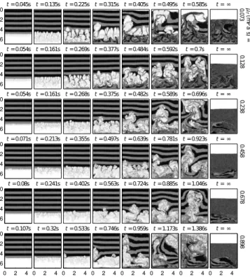
In Fig.7the influence of the fluid viscosityfis demon-strated in plots of the density field in black and white, where black stands for high particle density. Stripes in gray were added to emphasize the particle dynamics. The viscosity is changed from a value close to the viscosity of air f共air兲
FIG. 6. 共Color online兲 The averaged pressure profile as a func-tion of the depth at t = 0.02 s.
= 0.018 mPa s and increased in steps with increasing step size. When the viscosity is increased a clear difference in the dynamics in the cell can be observed. The structures get smaller and the evolution of the dynamics is slowed down. When the viscosity is increased, the fingers finally disperse before they have reached the base of the cell. In the further progress the most advanced bubble of low particle density accelerates until the top section of compacted grains has been broken through. After this breakthrough the top section gets unstable, and the remaining blocks of compacted grains remain compacted while falling downward. This is a rather different dynamics, where we have already observed that the friction with the side plates is an important parameter 关12兴.
The focus of this paper shall be kept on the start of the Rayleigh-Taylor instability, which is less sensitive to bound-ary conditions, and allows us to concentrate on the paramet-ric study of the viscosity and compressibility effects. Thus, we have chosen not to study in detail this final stage of the dynamics, and we concentrate on the beginning of the simu-lations when the top layer is still intact.
The analysis of the excess path length of Sec.III Ain Eq. 共12兲 performed on the simulations with different viscosities
leads to the plot in Fig.8. Here, we can see that the first 8000 particles follow a longer trajectory in relation to the move-ment of their centers of mass the more viscous is the fluid. There is no simple way to rescale all the plots and collapse them for all viscosities. This shows that the characteristics of the patterns in the density field and the dynamics of the particles are changed due to the viscosity.
To further analyze this change in the mixing dynamics, we define ⌬d as the average relative distance of particles pairs. These pairs were at time t = 0 s separated by a distance ⌬ds⬍0.028 cm, which corresponds to two particle diam-eters. In this average only the first 600 particles are consid-ered corresponding to the first two layers. The reason for this is that the front where particles disperse from the top section travels slower for higher viscosity, and the amount of
par-FIG. 8. 共Color online兲 The average excess particle trajectory in relation to the displacement of the center of mass.
FIG. 9. 共Color online兲 ⌬d the average distance of particle pairs in time for low-viscosity fluids in bilogarithmic representation. The power-law fit with an exponent b = 1.0 shows ballistic behavior.
FIG. 10.共Color online兲 ⌬d the average distance of particle pairs in time for high-viscosity fluids in bilogarithmic representation. The initial separation of the pairs has a diffusive behavior with an ex-ponent close to b = 0.5 in the dashed line. In the progress a crossover to a turbulent-dispersive behavior is observed with a slope close to b = 1.5 in the solid line.
FIG. 7. The particle density field of simulations with different viscosities. From left to right time is progressing, and from top to bottom the viscosity is increased. If not specified the axis units are given in centimeters. White areas represent particle-free areas. Bubbles of low particle density can be observed.
NIEBLING et al. PHYSICAL REVIEW E 82, 051302共2010兲
ticles that contribute to the averaged particle pair distance would depend on the speed the front travels with. Further-more the dynamic patterns in the cell also depend on the height from the bottom of the cell and coarsen in time. By taking the average over the first 600 particles, it can be en-sured that all the particles almost start moving instanta-neously. The analysis stops when the first particle has reached a distance of 0.14 cm to the base of the cell corre-sponding to ten particle diameters. The average distance be-tween the particle pairs grows in time while the particles are falling through the fluid as shown in the bilogarithmic rep-resentations in Figs. 9 and 10. The pair separation can be classified into two regimes. The first regime for lowly vis-cous fluids with 0.018ⱕfⱕ0.073 kPa s shows a nonhy-drodynamic or ballistic behavior where the exponent is close to b = 1.0 in a power-law fit of⌬d=atb. The particles in this regime fall with a constant relative velocity. In the second regime for highly viscous fluids with 0.128ⱕf ⱕ4.418 kPa s the particle pairs follow an initial diffusive separation with an exponent close to b = 0.5 before they enter the turbulent-dispersive behavior with an exponent close to
b = 1.5. Interestingly the latter exponent of b = 1.5
corre-sponds to the Richardson law that predicts an exponent of
b = 1.5 for particle pair separation in fully developed
turbu-lence 关20–24兴. For later stages this observation however
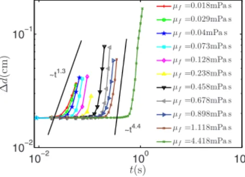
changes. Looking at a layer of 600 particles at a height of 2000 particles up in the packing, the pair separation displays a slope of around b = 3.6 for particles emerged in high-viscosity fluids共see Fig.11兲. The ballistic behavior for
par-ticles emerged in low-viscosity fluids is slightly more stable
and holds for a layer of 600 particles until a height of 4000 particles up in the packing 共see Fig. 12兲. In both plots the
slopes increase systematically with the fluid viscosity. In ad-dition to the coarsening of the dynamic pattern the more rugged interface at later stages can cause this behavior. The more rugged interface at later stages causes the particles to disperse from the compacted layer at different times and can also contribute to a higher slope of the pair separation in the bilogarithmic representation.
IV. CONCLUSION
As a conclusion we can state that the compressibility of the interstitial fluid affects the dynamical patterns much less than the viscosity. Under the conditions discussed in Sec.
III B that the skin depth of the pressure is larger than the system size and that the weight of the grains does not lead to a significant compression of the fluid in the empty zone of the cell, the compressibility can be neglected. This results in an increase in the computational speed by a factor of around 20 for the present model from 480 to 24 h on a cluster with eight nodes. In the second part of this paper the viscosity was proven to have a strong effect on the dynamics of the par-ticles. In terms of the mixing behavior the increase in the additional path length due to the increase in the fluid viscos-ity will result in a better mixing of the particles the more viscous the fluid is if internal friction is negligible. For some regions in the flow next to the initial fluid-grain pack bound-ary, a transient power-law behavior is observed for the de-pendence on time of particle pair separation. The exponent characterizing these power laws is observed to increase as a function of the fluid viscosity.
关1兴 P. Tegzes, T. Vicsek, and P. Schiffer, Phys. Rev. Lett. 89, 094301共2002兲.
关2兴 R. M. Iverson, M. Logan, and R. P. Denlinger, J. Geophys. Res. 109, F01015共2004兲.
关3兴 R. P. Denlinger and R. M. Iverson, J. Geophys. Res. 109, F01014共2004兲.
关4兴 J. Duran and A. Reisinger, Sands, Powders, and Grains: An
Introduction to the Physics of Granular Materials 共Springer-Verlag, New York, 1999兲.
关5兴 L. Bergougnoux, S. Ghicini, E. Guazzelli, and J. E. Hinch,
Phys. Fluids 15, 1875共2003兲.
关6兴 E. Guazzelli,Phys. Fluids 13, 1537共2001兲.
关7兴 H. Nicolai, B. Herzhaft, E. J. Hinch, L. Oger, and E. Guazzelli,
Phys. Fluids 7, 12共1995兲. 10−2 100 102 10−2 10−1 100 t(s) ∆ d (cm ) µf=0.018mPa s µf=0.029mPa s µf=0.04mPa s µf=0.073mPa s µf=0.128mPa s µf=0.238mPa s µf=0.458mPa s µf=0.678mPa s µf=0.898mPa s µf=1.118mPa s µf=4.418mPa s ~t3.6 ~t1.0
FIG. 11. 共Color online兲 Bilogarithmic representation of ⌬d, the average distance of particle pairs in time, for a layer of 600 particles at a height of 2000 particles up in the packing. The slopes increase systematically with the fluid viscosity.
10−2 100 102 10−2 10−1 t(s) ∆ d (cm ) µf=0.018mPa s µf=0.029mPa s µf=0.04mPa s µf=0.073mPa s µf=0.128mPa s µf=0.238mPa s µf=0.458mPa s µf=0.678mPa s µf=0.898mPa s µf=1.118mPa s µf=4.418mPa s ~t1.3 ~t4.4
FIG. 12. 共Color online兲 Bilogarithmic representation of ⌬d, the average distance of particle pairs in time, for a layer of 600 particles at a height of 4000 particles up in the packing.
关8兴 H. Nicolai and E. Guazzelli,Phys. Fluids 7, 3共1995兲.
关9兴 J. L. Vinningland, Ø. Johnsen, E. G. Flekkøy, R. Toussaint, and K. J. Måløy,Phys. Rev. Lett. 99, 048001共2007兲.
关10兴 J. L. Vinningland, Ø. Johnsen, E. G. Flekkøy, R. Toussaint, and K. J. Måløy,Phys. Rev. E 76, 051306共2007兲.
关11兴 J. L. Vinningland, Ø. Johnsen, E. G. Flekkøy, R. Toussaint, and K. J. Måløy,Phys. Rev. E 81, 041308共2010兲.
关12兴 M. J. Niebling, E. G. Flekkøy, K. J. Måløy, and R. Toussaint,
Phys. Rev. E 82, 011301共2010兲.
关13兴 Ø. Johnsen, R. Toussaint, K. J. Måløy, and E. G. Flekkøy,
Phys. Rev. E 74, 011301共2006兲.
关14兴 Ø. Johnsen, C. Chevalier, A. Lindner, R. Toussaint, E. Clé-ment, K. J. Måløy, E. G. Flekkøy, and J. Schmittbuhl,Phys. Rev. E 78, 051302共2008兲.
关15兴 S. McNamara, E. G. Flekkøy, and K. J. Måløy,Phys. Rev. E
61, 4054共2000兲.
关16兴 D.-V. Anghel, M. Strauss, S. McNamara, E. G. Flekkøy, and K. J. Måløy,Phys. Rev. E 74, 029906共E兲 共2006兲.
关17兴 P. C. Carman,Chem. Eng. Res. Des. 75, S32共1997兲.
关18兴 E. G. Flekkøy, R. Delgado-Buscalioni, and P. V. Coveney,
Phys. Rev. E 72, 026703共2005兲.
关19兴 W. H. Press and W. T. Vetterling, Numerical Recipes 共Cam-bridge University Press, Cam共Cam-bridge, England, 2002兲. 关20兴 L. F. Richardson, Proc. R. Soc. London, Ser. A 110, 709
共1926兲.
关21兴 T. H. Dupree,Phys. Fluids 9, 1773共1966兲.
关22兴 T. H. Dupree,Phys. Fluids 15, 334共1972兲.
关23兴 G. Boffetta, A. Celani, A. Crisanti, and A. Vulpiani,EPL 46, 177共1999兲.
关24兴 J. H. Misguich and R. Balescu,Plasma Phys. 24, 289共1982兲.
NIEBLING et al. PHYSICAL REVIEW E 82, 051302共2010兲