Propagation of electromagnetic waves through the Martian ionosphere

HAL Id: insu-03234946

https://hal-insu.archives-ouvertes.fr/insu-03234946

Submitted on 25 May 2021

HAL is a multi-disciplinary open access

archive for the deposit and dissemination of

sci-entific research documents, whether they are

pub-lished or not. The documents may come from

teaching and research institutions in France or

abroad, or from public or private research centers.

L’archive ouverte pluridisciplinaire HAL, est

destinée au dépôt et à la diffusion de documents

scientifiques de niveau recherche, publiés ou non,

émanant des établissements d’enseignement et de

recherche français ou étrangers, des laboratoires

publics ou privés.

Propagation of electromagnetic waves through the

Martian ionosphere

Olga Melnik, Michel Parrot

To cite this version:

Olga Melnik, Michel Parrot. Propagation of electromagnetic waves through the Martian ionosphere.

Journal of Geophysical Research Space Physics, American Geophysical Union/Wiley, 1999, 104 (A6),

pp.12705-12714. �10.1029/1999JA900100�. �insu-03234946�

JOURNAL OF GEOPHYSICAL RESEARCH, VOL. 104, NO. A6, PAGES 12,705-12,714, JUNE 1, 1999

Propagation of electromagnetic waves

through the Martian ionosphere

Olga Melnik and Michel Parrot

Laboratoire de Physique et Chimie de l'Environnement, Centre National de la Recherche Scientifique

Orl6ans, France

Abstract. This paper is related to the study of ELF-VLF wave propagation

through

the Martian

ionosphere

using a WKB method.

It is expected

that waves coming

from the atmosphere

could be

observed

by a probe in orbit around

Mars. Characteristics

of the wave propagation

have been

determined

from Maxwell's equations.

The ionospheric

conductivities

have been calculated

using

known parameters

of the Martian ionosphere

in different

cases:

nightside

and dayside,

low and

high solar activity, and low and high magnetic

field. It is shown

that ELF-VLF waves

with a

maximum

frequency

- 4000 Hz can only propagate

if we consider

a strong

magnetic

field on the

nightside

and a low solar activity.

1. Introduction

The Martian atmosphere is too tenuous to have lightning as on the Earth. But electrical discharge may occur in the large dust and sand storms which exist on this planet. In a previous paper, Melnik and

Parrot [1998] showed with a numerical simulation that such events

are possible. When it occurs, this electrical discharge is able to generate electromagnetic waves in a broad frequency range. As waves can propagate in the atmosphere and then in the ionosphere, it could be possible to observe these emissions with a probe in a low orbit around Mars. However, attenuation or even complete reflection of the waves could occur in the ionosphere depending on the wave frequencies and on plasma parameters. The purpose of this paper is to check the propagation characteristics of these electromagnetic waves through the Martian ionosphere using a WKB method. The approach to investigate the problem is similar to

the work of Huba and Rowland [1993] who studied the wave

propagation through the ionosphere of Venus.

The analytical expression of the wave dispersion relation is calculated in section 2. Section 3 presents the variations of the ionospheric parameters which have been obtained from a search of the literature in order to numerically evaluate the dispersion relation. Simplified solutions for specific frequency ranges are given in section 4, whereas the main results are shown in section 5. Finally, conclusions are given in section 6.

2. Dispersion Relation

The equations for the electric field E and for the magnetic field B

are derived from the Maxwell equations'

0B - -VxE 0t

l aE

(1)

- Vx B - la

0j : Vx B - la0ooE

Copyright 1999 by the American Geophysical Union. Paper number 1999JA900100.

lo i 48-0227/99/i 999JA900 i 00509.00

where the first equation is Faraday's law and the second is Ampere's law; c is the velocity of light, [t o is the permeability of free space, and o is the conductivity tensor (see appendix A). We will consider an orthogonal Cartesian coordinate system (x, y, z) where the z axis is vertical. The Martian magnetic field B 0 is directed toward the z direction, and we will study the propagation of waves parallel to B 0, i.e., with a wave normal along the z axis. Then the transverse field

can be written as

E = ExX + Evy

B : B

x x + By

y

(2)

The temporal

and spatial

variations

of the components

E x , E¾,

B•,

and By are o< exp i((0t - kz), where (0 is the angular frequency and k

is the wave number. Relative to the electric components and using the components of the conductivity tensor (see appendix A, equation (A2)), equation (1) can be written as

(02

(7 - k2 _ i(0g0op)E•

- i(0g0oH

Ey = 0

(--•-

- k2 _ i (01a

o

O

p

) Ey

+ i (01a

o

o

u E

x = 0

(3)

Using the complex thnction F_. = E x ñ iEv, equation (3) can be

written in the simplified/brm:

032

[-•- - k 2 - (0go(io•,•+or•)lF._

= 0

(4)

With ½01&c2

= 1, the dispersion

relation

becomes

12,705

(02 1

12,706 MELNIK AND PARROT: EM WAVES IN THE MARTIAN IONOSPHERE

We will only study the case of the right mode waves F+ which will be written F in the following sections. In a two-component plasma,

the conductivities

•, and a n depend

on the collision

frequencies,

the

gyrofrequency. Their analytical expressions are given in appendix A. The quantities needed to evaluate the conductivities are given in section 3.

3. Martian Ionospheric Parameters

The wave propagation has been studied during low and high solar

activity and for the dayside and nightside of the ionosphere. The relevant ionospheric parameters are obtained from experimental

results (Mariner, Viking) or from models. Neutral densities are given by Winchester and Rees [1995] and Fox et al. [1996]. The densities are measured during low solar activity and on the dayside.

In the absence of other measurements, we used these values for all

cases. The total neutral density in the altitude range we survey is

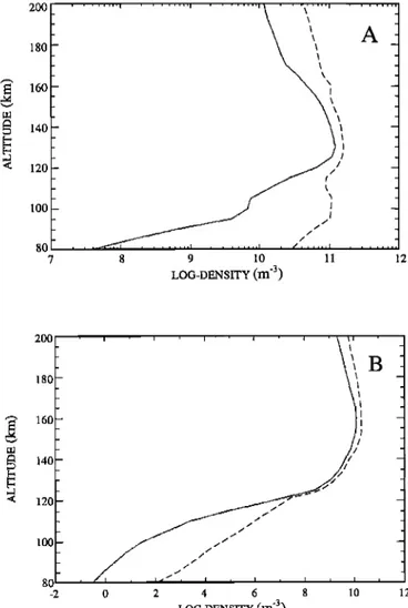
given in Figure 1. Densities of major ions on the dayside and during

a low solar activity have been presented by Shinagawa and Cravens [1989], Winchester and Rees [1995], and Fox et al. [1996]. The same parameters during a high solar activity have been obtained by Fox et al. [1996]. Densities of major ions on the nightside and during low and high solar activity are given by Haider [ 1997] and

Fox et ai. [1993], respectively. In the following, we will assume that

we have equilibrium, i.e., the sum of the ion densities is equal to the electron density in all cases. Figure 2 represents the total ion density as a function of altitude. In Figure 2a, the solid line and the dashed line are related to a low and high solar activity, respectively, on the dayside, whereas the same curves in Figure 2b are related to data on the nightside. The values are in agreement with the electron densities provided by Fox et al. [1996] for low and high solar activity on the dayside and by Haider [1997] for a low solar activity on the nightside. The electron temperature data, which are adapted from Fox et al. [1996], are represented in Figure 3.

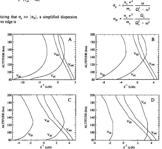
Therefore, using data of Figures 1-3, the collision frequencies given by (A7) can be evaluated for the different conditions. They are represented in Figure 4.

Two models of the Martian magnetic field have been used. They are plotted in Figure 5. Figure 5a shows an adaption of the induced magnetic field calculated by Shinagawa and Cravens [1989], whereas Figure 5b shows a field variation extrapolated from the recent measurement from Mars Global Surveyor by Acuga et al. [ 1998]. They have shown that the intrinsic Martian magnetic field

2OO 180 160 140 120 100

A

LOG-DENSITY

(m '3)

• 140

//

-

LOC-VENSrr¾

(m

'3)

Figure 2. Total ion density as a function of altitude. The solid line and the dashed line are related to a low and high solar activity, respectively, on (a) the dayside and (b) the nightside.

12

could be as high as 400 nT at some locations. As examples, the

gyrofrequency of the ion O + which is considered as the main ion in

this study, the electron gyro-frequency, and the plasma frequency

COpe

= (nee2/½omO

m (see

appendix

A) are

plotted

in Figure

6 for

the

nightside and during low solar activity. Figure 6a is related to the magnetic field shown in Figure 5a, whereas Figure 6b is related to the field shown in Figure 5b.

200 180

160

14

15

'i6

Figure 1. Total neutral density as a function of altitude.

4. Approximate Solutions

Figures 4 and 5 define eight different cases, and, in a first time, rough solutions can be evaluated to determine if propagation is possible.

4.1. Low Solar Activity and on the Nightside

Approximate values of the conductivities (A6) are calculated for a low solar activity, and on the nightside, in order to obtain rough solutions of the wave equation (4) in given frequency ranges. 4.1.1. Induced magnetic field. This case corresponds to Figures 4a and 6a. At the lower edge, it is observed that v•,, >> v•i, vi•, that v•,,

MELNIK AND PARROT: EM WAVES IN THE MARTIAN IONOSPHERE 12,707 200 I80 160

140

19-0

lOO

Temperature

(K)

Figure 3. Electron temperature as a function of altitude.

>> Ifl•l, and that f•,,[ >> f•i. Then, the equations

(A6) can be

written O -- O H = 2 II e e ] m e (re. + i(0)

•

(6)

n e e

f•e

me (v•n + i(0)2

From (5) and noticing

that %, >> Ion, a simplified

dispersion

2

k 2 = (02

_c

₂

_[1

_{- i •P•- ]}

₍₇₎

(0 (re.+ i(0)

The condition (0 << v,,, in equation (7) gives

2

N

2 = 1 - i com

(8)

(0 Ven

where N is the refractive index (kc/(0). Equation (8) shows that waves are attenuated when they propagate from the lower ionosphere up to altitudes where the ionization and the magnetic

field play essential roles. In the opposite case, (0 >> yen, we have

2

/v==

1 - %'•

(9)

and the waves are propagating without attenuation.

At higher altitudes (> 120 km), the plasma frequency is larger and we can expect a large attenuation of waves propagating in the whistler mode. The collision frequencies are roughly of the same

order

(ve,,- Vii

, '"'

Vei)

and IC•l >> v•.

With the condition

(0 >>v=,,

the conductivities

become

2 .lIe e p

m

e f• _ (02

lIe e2

f•e

m

e f• _ (02

(lO)

180

I

140

200 ...

₁₈₀

•

200 ....

₁₈₀

•

_V

_e

_{i D}

,

• [ ) Vin•• I

Vin

100

Ven 100

Figure

4. Collision

frequencies

v• as a function

of altitude

(i ion; e electron;

n neutral)

during

(a) low solar

activity

12,708 MELNIK AND PARROT: EM WAVES IN THE MARTIAN IONOSPHERE 20O 150 A

0

1•0

2•

3•

40

Figure 5. Magnetic field as a function of altitude. (a) Inducted magnetic field adapted from Shinagawa and Cravens [ 1989] and (b)

intrinsic magnetic field (see text).

The Pedersen conductivity is purely imaginary and the Hall

conductivity is purely real. The refractive index is

2

N 2= 1 -

tope

•O(•O

* •)

(1

1)

The waves

can

propagate

in the frequency

band

v=•

<< to < f• as

it is expected. For high frequency (to >> f• ), the refractive index,

which is given by (9), indicates that the propagation is possible for

waves

with to > top,,

as usual.

When the frequencies

are lower and

similar to the collision frequencies v ... ; the propagation is

impossible. In this case (induced magnetic field, low solar activity, and nightside), there is no propagation because the refractive index at the lower edge of the ionosphere is given by (8).

4.1.2. Intrinsic magnetic field. This case corresponds to Figures 4a and 6b. At the lower edge, we have the conditions v•,, >> v•;.,• and

f•, > v•,,' the conductivities are

O H -

n e e 2

Ven

*

m• • + (v•n + ito)2

n e e

m• f• + (v•. + ito)2

and then, if to << v .... the refractive index is

2

N

2= 1 -

(13)

to(O¾

- ivy,,)

which means that the waves can propagate with little attenuation in

the layers where the approximation is valid. When the frequencies are equal to the collision frequencies between neutral and charged particles, the attenuation is preponderant.

For the ionospheric layers between -120 km and -170 km, the

refractive index is given by equation (11). The waves with

frequencies

to >> v=• are propagating

with little attenuation.

The

waves

with lower

frequencies

(to-v•o)

are more

attenuated.

2OOL ( ' . 180 .

160

14o

/

100

/

/

180

1

160

•

....

///

Figure 6. Representation

of the O + gyrofrequency

f•i, the electron

gyrofrequency

f• , and the plasma

fequency

top•

as function

of

MELNIK AND PARROT: EM WAVES IN THE MARTIAN IONOSPHERE 12,709

In the upper ionosphere, the collision frequencies decrease, and

equation

(11) is valid

in the frequency

range

v• (( to ( f•e ß

The

4.2. Other Cases

Figure 4b, which concerns the case "high solar activity and on the nightside", is very similar to Figure 4a, and therefore the conditions for propagation described in sections 4.1.1 and 4.1.2 are valid. Propagation is only possible when the magnetic field is strong enough.

On the dayside, ionization is much more important than on the nightside and the collision frequencies between charged particles

increase as it is seen in Figures 4c (low solar activity) and 4d (high solar activity). Therefore the same case as in section 4.1.1 but on the

dayside corresponds to a worse situation because vei- Ifl•l between

90 and 140 km. For a strong magnetic field, the propagation during

low solar activity is also not possible because the condition re,, >>

v•i used in section 4.1.1, is only valid at the lower edge of the ionosphere. The conditions of propagation relative to the case "high solar activity and on the dayside" (Figure 4d) are much more unfavorable than during low solar activity whatever is the intensity of the magnetic field.

5. Results

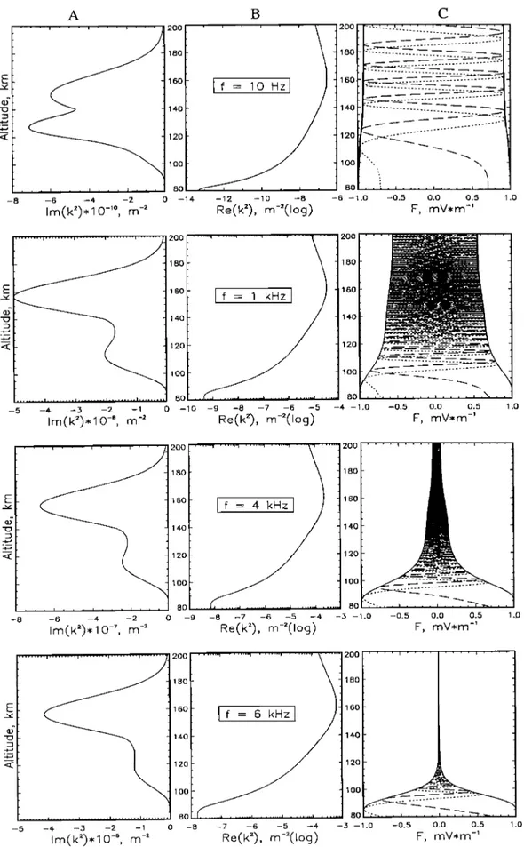
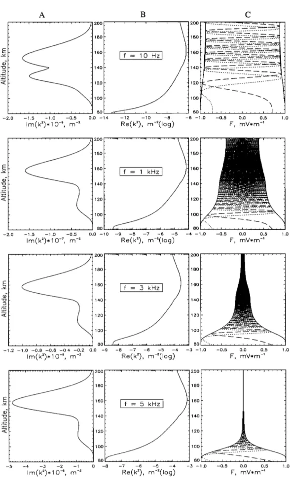
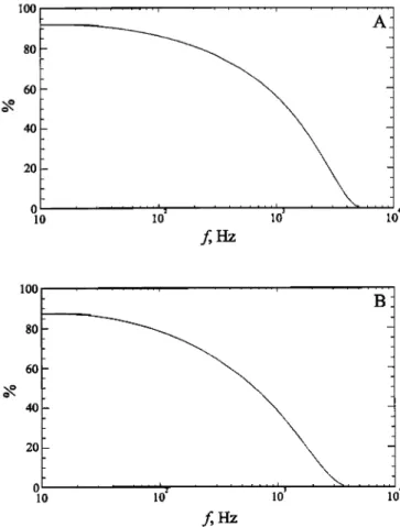
For HF waves with frequency larger than the plasma frequency, there is no propagation problem. However, considering the approximations of the solutions in different cases which are detailed in section 4, it is clear that the ELF-VLF wave propagation will only occur on the nightside and when the magnetic field is strong enough. The solution of equation (4) is given in appendix B. We studied waves in a frequency range from 10 Hz to 10 kHz. The results for the nightside case with a strong magnetic field and a low solar activity are shown in Figure 7. The imaginary part and the real part of the square of the wave number amplitude are shown for different frequencies in Figures 7a and 7b, respectively. A condition to have small wave attenuation is that the real part of the amplitude of the wave number k is much larger than the imaginary part. Figure 7c represents the wave amplitude for different frequencies. The dashed, dotted, and solid lines represent the real part, the imaginary part, and the modulus of F as function of altitude, respectively. To plot the curves, we have chosen at 80 krn an arbitrary value of the wave modulus A equal to 1 mV/m in the system of equations (B9). At f = 10 Hz, it is shown that the wave propagates without attenuation up to 120 km but that it suffers moderate attenuation above 120 km. At higher frequencies (from - 100 Hz up to - 5 kHz), the wave amplitude is also reduced but can reach the topside ionosphere. When the frequency is larger than 6 kHz, the waves are entirely attenuated in the first ionospheric layers. Figure 8 is similar to Figure 7, but it concerns the case of high solar activity. It can be

observed that the features are more or less identical with the

following differences: (1) The maximum frequency of waves reaching the topside ionosphere is smaller and (2) for a given frequency, the amplitude of the waves at 200 km is smaller than in the previous case. These two points are detailed in Figure 9, which shows the percentage of the wave amplitude for waves reaching the ,u.osp.c•c as a function of frequency Figure 9a is related

tOp•lu• .

to Figure 7 (low solar activity), whereas Figure 9b is related to Figure 8 (high solar activity). In the two cases, the percentage decreases slowly with the frequency but with a slope which is

slightly different (at 1 kHz for example, the attenuation is - 56% for

the low solar activity, whereas it is - 38% for the high solar activity). It is confirmed that the maximum frequency of

propagating waves is larger for low solar activity (- 4000 Hz).

The validity of the WKB approximation is discussed in appendix B, and application of equation (B 10) to the above eases indicates

that problems could appear for frequencies < 100 Hz between 80

and 100 kin. It is the lower edge of our analysis domain, and then the WKB method used to study the wave propagation has no implication on the results.

6. Conclusions

The propagation of ELF-VLF electromagnetic waves through the Martian ionosphere has been investigated. This work used the ionospheric parameters which have been measured during past experiments or obtained with models. It shows that if we consider a low magnetic field induced by the solar wind, no propagation of waves from the atmosphere up to the top ionosphere would be possible. The waves will only propagate through the ionosphere if the Martian magnetic field is strong enough. The probe Mars Global Surveyor has shown that such high value could occur above specific regions of the Martian surface. In such a case we have shown that the waves can propagate on the nightside. The frequency window is larger and the amplitude attenuation is lower during low solar activity than during high solar activity. Waves with frequencies less than 4 kHz are able to go through the ionosphere during low solar activity. Their attenuation is frequency dependent. We assume in our calculations that the ionosphere is uniform. In the case of ionospheric irregularities, propagation is always possible in guides.

For simplicity, the special case of propagation along the magnetic field has been considered. It is expected that oblique waves will be more strongly attenuated because of their longer ray paths in the collisional ionospheric layers.

This work was undertaken as part of the wave experiment ELISMA on board the MARS 96 wission [ELISMA Experimenters, 1998]. The main scientific objective of ELISMA was to study the electromagnetic waves in the Martian ionosphere, but, unfortunately, the launch of MARS 96 failed. Another wave experiment has been recently launched onboard the Japanese mission PLANET-B [Tsuruda et al., 1996].

Another application of this study is related to the possibility of

using HF radio on Mars. In the future, communications between several bases on the surface of Mars may be needed without the

help of an orbiter [Fry and Yowell, 1994], and working frequency

for these must be chosen. Waves with frequencies larger than the plasma frequency will not be reflected by the ionosphere. The maximum values of the plasma frequency are - 0.9, 1.2, 2.7, and 3.7 MHz for the nightside during low solar activity, the nightside

during high solar activity, the day side during low solar activity, and

the dayside during high solar activity, respectively.

Appendix A: Conductivity Tensor

Ohm's law with an electric field E can be written as

12,'710

MELNIK

AND PARROT:

EM WAVES

IN THE MARTIAN

IONOSPHERE

A

B

C

'

... I . •)

I , 1

--8 --6 --4. --2 0 --14 --12 --10 --8 --6 --1.0 --0.5 0.0 0.5 .0

Im(k').10 -'ø, m-'

Re(k'), m-'(Iog)

F, mV.m-'

... , ... , ... , ... , ... 200 ... '• ... " ... ' ... • ... 2 C 180 I .C,

•

160 f = 1 kHz

C_ t1øf

f

_...ql0o

f

r

,

, •• ... , ...

i 80/

Im(k')*10-', m-'

Re(k'), m-'(Iocj)

F, mV.m-'

, , , ! , , , • , , , ! , , , ii

.

•-•-m-

"•

11

-

, , , i , , , • , , , • , ß ß

-8 --6 --4 --2 0 --9 --8 --7 -6 -5 --4 -3 --1.0 --0.5 0.0 0.5 1.0

Im(k2).10

-', m-'

Re(k;'),

m-;'(Iog)

F, mV.m-"

i ...

i

...

i

...

I

...

i

...

Im(k•).10 -•, m -•

Re(k'), m-'(Iog)

Figure

7. Wave

number

and

wave

amplitudes

as

function

of altitude

for different

frequencies,

for the

nightside

case

with a strong

magnetic

field, and

a low solar

activity.

(a) The imaginary

part

of the square

of the wave

number

amplitude.

(b) The

real

part

of the

square

of the

wave

number

amplitude.

(c) The

wave

amplitude

(the

dashed,

dotted

and

solid

lines

represent

the real part,

the imaginary

part,

and

the

modulus

of F, respectively).

MELNIK AND PARROT: EM WAVES IN THE MARTIAN IONOSPHERE 12,'711 A B C

i'

1

1

Im(k2).10 -9

, m -2

Re(k2), m-•(Iog)

f

t1øf

\]1,

[:2 [,_ • -[ 160[- ...

1 40 1

•" 120 1

f •100f

•

-LO ' '

'1'-

''.

'-5 1

• I•'

'. '-0.'•'

' '010

80-[1C•"f'"'J9

...

JIB

...

J7

...

J6''"•-5

...

•4 1

0

•m(k')*•O-', m -•

•(k•),

•-•(•og)

[:[- •

-]16o[- If = ,3 kHz

I

} -[1

il •

11401 / 11

•f

Q•.

]12o

F

•

]1

'tlOOF

t 1

f,., ,, _ ,,,, ,,,. •,., ,... I 801

...

I,., ....

, ...

, ., ... .• ...

•m(•=)-•o-', m -=

•(•),

m-=(•og)

•m(•),•o -", m -•

•(•),

m-=(Iog)

F, mY*m-'

12,712 MELNIK AND PARROT: EM WAVES IN TttE MARTIAN IONOSPHERE lOO 80 60 20 o lO lO lO lO Z Hz

a and 13 (e electrons, i ions, and n neutrals). We assume that the temporal variation of the electron velocity v• and the ion velocity v i is • exp(irot) where ro is the angular frequency. Therefore, using (A3), the equations for the velocity components transverse to the

magnetic field are

E• K1 Ev K2

E• K2 Ey K1

Vex

=

• ('-•-)+

• ('-•-)

Vey=

• (-'-•-)

+

--(--•-)

B 0

E•

. K3

) + Ev

K4

• K4 Ey

. K3

)

V•=m(Ct

• •(•)Viy=•(-•)+•(•

(A4)

10

10

0

10'

Figure 9. Percentage of the wave amplitude transmitted from 80 to

200 km as function of frequency during (a) low solar activity and (b) high solar activity.

where j is the current induced by E. The conductivity tensor o is

O/, O

H 0

-O

H Op 0

0

0 %

(A2)

where

D = (f•2 + Ae2)(•i2

+ Ai2)+(ArJ•i_VeiVie)2

+ 2•e•iVeiVie;

K1 =

(•fi•-i

+ •iv,.i)(A,J•-,

- v,.ivi•)

+ •Q,2(Ae

- v,.i);

K2 = •e2(Ai

2 + [•'•/2)

+

['-•e•'•iVei(Ai

+ Vie

) q- ['-•i2AeVei;

K3 = (•iA.. + ['-•eVie)(A.J•

i - VeiVie)

q-

f•2•,(A

i - %); K4 = •i2(Ae2

+ •e 2) + •e•iVie(Ae

+ Vei)

+ •e2Aivie;

A e

= v,,,,

+vei

+ iro and A i = vi,, + v•,,

+ ioa.

The usual

electron

and

ion

gyrofrequencies

are respectively

given by l e[Bdm• and [•'•i

----

q•

Bo/m •, but it must be noted that in all equations and in the calculation of the conductivities, f• = eBo/m • and must be

considered as a negative quantity. Using (A1), the components of the current can be written on the following form:

j• = op

E•

+ o

n El,

= n•

e (V•x

- V/x) (A5)

jy = op •, - 0 n E• = n• e (vo, - Viy

)

where n• is the electron density. Then, combining (A5) with (A4),

one obtains the Pedersen and the Hall conductivities:

n•e (A,,A

i -["•e•'•i-

VeiVie)(•'•i(Vei

-A•) -["•e(Vie

-Ai))

O H -

B (f•2 + Ae2)(•-•i2

+ Ai2)

+(A•Ai-

VeiVie

)2 + 2f•e•'•iVeiVie

(A6)

n•e •e2Ai

2 -•i2Ae2-

(•e¾ie-•iYei)(•eAi

+ f•iA•,))

B (f•2 + Ae2)(•i2

+ Ai2)+(AeAi_

¾ei¾ie)2

+ 2•e•iVeiVi

e

The collision

frequencies

v•o are given

by the usual

formulae

[Rishbeth and Garriott, 1969; Ratcliffe, 1972; Kelley, 1989]'

where

the three

parameters,

%, op, and o• are called

the specific,

motion for electrons and ions under the action of the Coulomb and

Lorentz forces and in the presence of collisions are written [Huba and Rowland, 1993]'

v,,,,

= 2.12 10-16

/•, T 1/2 s - l

vi,= 2.6 10-15

n, M1/2 s-1

v•i = 3.62 10

-6 n i Te

-312

ln(A) s

-•

(A7)

-

[E + VeXBo]

- Ve. V e - Vei (Ve-Vi)

O t

0¾i qi

(A3)

-

[E + vixBo] - Vin V

i - Vie (Vi-Ve)

Ot

m i

where

A = 1.23 10

7 re

3/2n•

-•/2,

% is the neutral

density,

n; is the

ion

density, T• is the electron temperature in K, and M is the mean

molecular weight of the ions.

Appendix B: Calculation of the Wave Field

respectively, q• and m• are the charge and the mass of ions,

respectively,

and

v,o

is the collision

frequency

between

the species

Appendix B presents the solution of equation (4) for the right

mode. The first derivative of the F function ( F is • exp i(rot- kz)) along the z axis is

MELNIK AND PARROT: EM WAVES IN THE MARTIAN IONOSPHERE 12,713

0

5 _ F•,i

- F•_

t = -ik.

F.

(B

1)

where j is the step index. Then we have the relation:

-Fj + 2ikj+lAZ

5+ 1 + 5+

2 = 0, j = 0, 1

... n-2 (B2)

dl 1 0 0 ... 0

-1 d 2 1 0 ... 0

0 -1 d• 1 ... 0

0 0 -1 d4 ... 0

0 0 0 ... 1 d,

F 2

F 3

r4

(B9)

If we suppose that a wave with an amplitude A is emitted at the lowest frontier of our system (z = 80 km), the above equation for j

= 0 can be written as

2ikiAz

Fi + F 2 : A

(B3)

The condition at the highest level supposes an outgoing wave when z > 200 km, and using the second derivative of F gives

02Fj

_ F•+i

- 2

5 + Fj_i

: _k.2F.

02z

2

Az 2

J •

(B4)

from which we have, for j = n:

F,_i + (knAz

2 - 2)F

n+ Fn l = 0

(B5)

The WKB solution for F can be expressed as [Yeh and Liu, 1972;

Stix, 1992]

z

F(z)

= k(z)-l/2exp(-i

f k(z)dz)

(B6)

o

If we take the ratio F,,+i/F,,, we find that:

k,, k +

F,+l

= • exp(-iAz."

) F,, (g7)

Then using (B5), the last equation of our system which gives the relation between F,, 4 and F n is

F,_•

+[k,2Az2-2+ exp(--iAz

)]F, =0 (B8)

With (B2), (B3), and (B8), we have the following tridiagonal matrix •qua.u, •uouam the u,u.,,uw,l/•1,/•2,/•3, '", /•n;

where

the complex

coefficients

dj are

given

by

•. = 2ik•Az for j = 1 ... n-1

• k. kn

+

kn+

1

d.

= k 2Az2

- 2 + • exp(-iAz .)

To solve (B9) between 80 and 200 km, we have chosen Az = 50 m

and then N = 2401.

The WKB approximation is valid if the variations of the plasma parameters (and then the variation of k) on a distance equal to the wavelength are small. This can be expressed by the following

inequality [Swanson, 1989]:

1 dkl

<<

1

(B

10)

Acknowledgment. Michel Blanc thanks both referees for their assistance in evaluating this paper.

References

Acufia, M.H., et al., Magnetic field and plasma observations at Mars: Initial results of the Mars Global Surveyor mission, Science, 279, 1676-1680, 1998.

ELISMA Experimenters, The wave complex on the MARS96

orbiter: ELISMA, Planet. Space Sci., 46, 701-713, 1998.

Fox, J.L., J.F. Brannon, and H.S. Porter, Upper limits to the nightside ionosphere of Mars. Geophys. Res. Lett., 20, 1391-

1394, 1993.

Fox, J.L., P. Zhou, and S.W. Bougher, The Martian

thermosphere/ionosphere at high and low solar activities, Adv. Space Res., 17, ( 11 )203-(11 )218, 1996.

Fry, C.D., and R.J. Yowell, HF radio on Mars, Communications Quarterly, 4(2), 13-23, 1994.

Haider, S.A., Chemistry of the nightside ionosphere of Mars, J.

Geophys. Res., 102,407-416, 1997.

Huba, J.D., and H.L. Rowland, Propagation of electromagnetic

waves parallel to the magnetic field in the nightside Venus ionosphere, J. Geophys. Res., 98, 5291-5300, 1993.

Kelley, M.C., The Earth's Ionosphere, Academic, San Diego, Calif., 1989.

Melnik, O., and M. Parrot, Electrostatic discharge in Martian dust

storms, J. Geophys. Res., 103, 29,109-29,117, 1998.

Ratcliffe, J.A., An Introduction to the Ionosphere and

Magnetosphere, Cambridge Univ. Press, New York, 1972.

Rishbeth, H., and O.K. Garriott, Introduction to Ionospheric

12,714 MELNIK AND PARROT: EM WAVES IN THE MARTIAN IONOSPHERE Shinagawa, H., and T.E. Cravens, A one-dimensional multispecies

magnetohydrodynamic model of the dayside ionosphere of Mars, J. Geophys. Res., 94, 6506-6516, 1989.

Stix, T.H., Waves in Plasmas, Am. Inst. of Phys., New York, 1992. Swanson, D.G., Plasma Waves, Academic, San Diego, Calif., 1989.

Tsuruda, K., I. Nakatani, and T, Yamamoto, Planet-B mission to

MARS-1998, Adv. Space Res., 17, (12)21-(12)29, 1996.

Winchester, C., and D. Rees, Numerical models of the Martian

coupled thermosphere and ionosphere, Adv. Space Res., 15, (4)51-(4)68, 1995.

Yeh, K.C., and C.H. Liu, Theory of Ionospheric Waves, International Geophysics Set., Academic, San Diego, Calif.,

1972.

O. Melnik and M. Parrot, Laboratoire de Physique et Chimie de l'Environnement, CNRS, 3A, Avenue de la Recherche Scientifique, 45071 Orldans cedex 02, France. (mparrot@cnrs-orleans.fr) (Received April 23, 1998; revised January 8, 1999; accepted February 5, 1999.)