Formulation of an ocean model for global climate simulations

(1)

HAL Id: hal-00298422

https://hal.archives-ouvertes.fr/hal-00298422

Submitted on 20 May 2005

HAL is a multi-disciplinary open access

archive for the deposit and dissemination of sci-entific research documents, whether they are pub-lished or not. The documents may come from teaching and research institutions in France or abroad, or from public or private research centers.

L’archive ouverte pluridisciplinaire HAL, est destinée au dépôt et à la diffusion de documents scientifiques de niveau recherche, publiés ou non, émanant des établissements d’enseignement et de recherche français ou étrangers, des laboratoires publics ou privés.

Formulation of an ocean model for global climate

simulations

S. M. Griﬀies, A. Gnanadesikan, K. W. Dixon, J. P. Dunne, R. Gerdes, M. J.

Harrison, A. Rosati, J. L. Russell, B. L. Samuels, M. J. Spelman, et al.

To cite this version:

S. M. Griﬀies, A. Gnanadesikan, K. W. Dixon, J. P. Dunne, R. Gerdes, et al.. Formulation of an ocean model for global climate simulations. Ocean Science Discussions, European Geosciences Union, 2005, 2 (3), pp.165-246. �hal-00298422�

(2)

OSD

2, 165–246, 2005

Formulation of an ocean climate model

S. M. Griffies et al. Title Page Abstract Introduction Conclusions References Tables Figures J I J I Back Close Full Screen / Esc

Print Version Interactive Discussion

EGU Ocean Science Discussions, 2, 165–246, 2005

www.ocean-science.net/osd/2/165/ SRef-ID: 1812-0822/osd/2005-2-165 European Geosciences Union

Ocean Science Discussions

Papers published in Ocean Science Discussions are under open-access review for the journal Ocean Science

Formulation of an ocean model for global

climate simulations

S. M. Griffies1, A. Gnanadesikan1, K. W. Dixon1, J. P. Dunne1, R. Gerdes2, M. J. Harrison1, A. Rosati1, J. L. Russell3, B. L. Samuels1, M. J. Spelman1, M. Winton1, and R. Zhang3

1

NOAA Geophysical Fluid Dynamics Laboratory, Princeton, USA

2

Alfred-Wegener-Institut f ¨ur Polar- und Meeresforschung, Bremerhaven, Germany

3

Program in Atmospheric and Oceanic Sciences, Princeton, USA

Received: 4 April 2005 – Accepted: 8 May 2005 – Published: 20 May 2005 Correspondence to: S. M. Griffies (stephen.griffies@noaa.gov)

(3)

OSD

2, 165–246, 2005

EGU

Abstract

This paper summarizes the formulation of the ocean component to the Geophysical Fluid Dynamics Laboratory’s (GFDL) coupled climate model used for the 4th IPCC As-sessment (AR4) of global climate change. In particular, it reviews elements of ocean climate models and how they are pieced together for use in a state-of-the-art coupled 5

model. Novel issues are also highlighted, with particular attention given to sensitivity of the coupled simulation to physical parameterizations and numerical methods. Features of the model described here include the following: (1) tripolar grid to resolve the Arctic Ocean without polar filtering, (2) partial bottom step representation of topography to better represent topographically influenced advective and wave processes, (3) more 10

accurate equation of state, (4) three-dimensional flux limited tracer advection to reduce overshoots and undershoots, (5) incorporation of regional climatological variability in shortwave penetration, (6) neutral physics parameterization for representation of the pathways of tracer transport, (7) staggered time stepping for tracer conservation and numerical efficiency, (8) anisotropic horizontal viscosities for representation of equato-15

rial currents, (9) parameterization of exchange with marginal seas, (10) incorporation of a free surface that accomodates a dynamic ice model and wave propagation, (11) transport of water across the ocean free surface to eliminate unphysical “virtual tracer flux” methods, (12) parameterization of tidal mixing on continental shelves.

1. Introduction

20

The purpose of this paper is to detail the formulation of the ocean model developed by scientists and engineers at NOAA’s Geophysical Fluid Dynamics Laboratory (GFDL) for use in our latest coupled global climate model. This paper is one in a series from GFDL, includingDelworth et al.(2005),Gnanadesikan et al.(2005),Wittenberg et al. (2005), andStouffer et al.(2005). The focus in the present paper is on the numerical 25

(4)

OSD

2, 165–246, 2005

EGU model component. Some of this paper takes the form of a review. We hope that this

format is useful for readers aiming to understand what is involved with constructing global models. We also highlight some novel scientific issues related to sensitivity of the coupled simulation to (1) the use of real water fluxes rather than virtual tracer fluxes, including the treatment of river runoff and exchange with semi-enclosed basins, (2) the 5

algorithm for time stepping the model equations, (3) sensitivity of the extra-tropical circulation to horizontal viscosity, and (4) treatment of the neutral physical parameteri-zations.

1.1. Documentation of ocean climate models

Many issues forming the fundamental elements of ocean climate models are often 10

briefly mentioned in papers primarily concerned with describing simulation characteris-tics, or they may be relegated to non-peer reviewed technical reports. Such discussions often leave the reader with little intellectual or practical appreciation for the difficult and critical choices made during model development. Our goal here is to partially remedy this situation by focusing on numerical and physical details of the most recent GFDL 15

ocean climate model. In so doing, we expose some of the guts of the model and at-tempt to rationalize choices. Along the way, we identify places where further research and development may be warranted.

This paper is written on the premise that the evolution of ocean climate science is facilitated by a candid peer-reviewed discussion of the interdependent and nontrivial 20

choices that developers make in constructing global climate models. The importance of such discussions has grown during the past decade as the models are used for an increasing variety of applications, many of which, such as climate change projections, garner intense scrutiny from non-scientific communities. Additionally, full disclosure is necessary for modelers to reproduce results of each other, and thus to enhance the 25

scientific robustness of climate modelling.

We admittedly fall short of fully realizing our goals in writing this paper. First, choices were made to balance conciseness with completeness. A substantially longer paper

(5)

OSD

2, 165–246, 2005

EGU with more thorough analysis of sensitivity experiments is required to satisfy the

com-pleteness goal. Some of these experiments will form the basis of separate studies. Second, we are limited by focusing on one particular climate model, that from GFDL contributing to AR4. Comparisons with other models go beyond the scope of this study, but such would certainly assist in understanding causes for the many differences found 5

in climate model simulations.

Given the above limitations, we remain hopeful that this paper serves as a step to-wards full disclosure of the rationale forming the basis for a particular ocean climate model. We believe such provides the climate science community with a useful re-source for understanding both how to reproduce elements of what we have done, and 10

to expose areas where further research and development is warranted. 1.2. Comments on ocean climate model development

One of the first global coupled climate models was that ofManabe and Bryan(1969). Their model used an early version of the GFDL geopotential vertical coordinate ocean model based on the work of Bryan and Cox (1967) and Bryan (1969b), with Bryan 15

(1969a) documenting algorithms used in this model. It is notable that such z-models, which typically employ the hydrostatic and Boussinesq approximations, still comprise the vast majority of ocean models used for climate simulations (see Griffies et al., 2000a, for a review). In particular, all versions of the GFDL coupled climate models to date have employed this class of ocean model.

20

In most z-models used for climate studies through the early 1990’s, the ocean prim-itive equations were discretized using spherical coordinates for the lateral directions, with vertical positions at fixed depths for all latitude and longitude points, and with grid cells of time independent volumes. Additionally, physical processes such as ocean tracer transport were aligned according to this grid. Since the middle 1990’s, there 25

have been fundamental advances to this older model formulation that significantly en-hance the physical integrity of z-model simulations (see Griffies et al., 2000a, for a review). It is therefore important to include these advances in the ocean climate

(6)

mod-OSD

2, 165–246, 2005

EGU els used for realistic climate simulations.

There are two main ways in which climate modellers seek realism in their simula-tions. First, the resultant simulation should behave like the observed climate. Second, individual physical processes should be represented or parameterized to the best of our understanding. As documented inDelworth et al.(2005),Wittenberg et al.(2005), 5

Stouffer et al.(2005), andGnanadesikan et al.(2005), the CM2 model series produces a climate that is relatively realistic in terms of its overall simulation. This document presents how we have addressed criticisms of previous GFDL models with regard to unrealistic representations of physical processes. We also highlight algorithm features that can result in significant changes in the model efficiency, stability, and simulation 10

characteristics.

1.3. Models discussed in this paper

Throughout this paper, we focus on two versions of the latest GFDL coupled climate model: CM2.0 and CM2.1. These versions have corresponding ocean model versions denoted OM3.0 and OM3.1. The model versions differ in the following ways.

15

The first difference is in the atmospheric component. CM2.0 uses a B-grid dynami-cal core documented byAnderson et al.(2005). CM2.1 uses the finite volume core of Lin(2004). Both atmospheric models use similar physical parameterizations. As dis-cussed inDelworth et al.(2005), the mid-latitude storm tracks in both hemispheres are shifted poleward in CM2.1 relative to CM2.0, with the largest shift (order 3–4◦) in the 20

Southern Hemisphere. This wind shift causes a nontrivial change in the ocean circula-tion in both hemispheres that significantly reduces middle to high latitude ocean biases in CM2.1 relative to CM2.0 (seeDelworth et al.,2005;Gnanadesikan et al.,2005, for full discussion).

The second difference is in the ocean model, with motivation for these changes 25

provided in this paper. These differences are the following.

(7)

OSD

2, 165–246, 2005

EGU two time step tendency.

– OM3.1 uses a constant neutral diffusivity of 600m2s−1. OM3.0 uses a noncon-stant diffusivity equal to the skew diffusivity, and this diffusivity is generally less than the 600m2s−1used in OM3.1.

– OM3.0 uses five times larger background horizontal viscosity poleward of 20◦than 5

OM3.1.

1.4. Organization of this paper

This paper consists of two main sections along with an appendix. In Section 2, we summarize how various methods and parameterizations documented in other studies have been incorporated into our ocean climate model. This section represents a review 10

of certain elements of ocean climate modelling that have been found to be critical in the construction of our model. Section3focuses on experiences and methods that are novel to this work. In particular, Sect.3.1explores the issues involved with switching from the commonly used virtual tracer fluxes to real water forcing. We then discuss time stepping algorithms in Sect.3.2, where we highlight the fundamental benefits of 15

a newly implemented “time staggered” scheme. Neutral physics parameterizations are described in Sect.3.3, where we note the reasons for changing the subgrid scale (SGS) parameters mentioned above. Horizontal friction is presented in Sect.3.4, where we show the rather large sensitivity of the simulation to the reduction in extra-tropical vis-cosity. Section3.5details our method for exchanging water mass properties between 20

the open ocean and semi-enclosed basins, and Sect.3.6 presents our approach for inserting river runoff into the ocean model. Both topics require some novel considera-tions due to our use of real water fluxes rather than virtual tracer fluxes. We close the paper in Sect.4with general comments about ocean climate model development. An appendix of model equations is given to support many discussions in the main text. 25

(8)

OSD

2, 165–246, 2005

EGU

2. Elements of the ocean model based on other work

When constructing an ocean climate model, it is necessary to choose from amongst a multitude of possible numerical and physical methods. We present here a compendium of model features that have been documented in other studies which are essential elements to our ocean climate model. The main aim here is to motivate choices. 5

Our discussion of choices made in this section is arguably brief. We are at fault, for example, for not providing illustrations of the sensitivity of our model to alternative choices. For example, when describing the model’s tripolar gridding of the sphere in Sect. 2.1, we argue for its benefits over the more traditional spherical grid. Yet we do not provide a direct comparison of simulations with and without the tripolar grid. 10

Instead, this choice, and many others, are based on the judgement and experience of the developers. Thorough model sensitivity experiments and analysis are not available to justify every model choice. Human, computer, and time limitations preclude such. Nonetheless, these choices are acknowledged, as they are important for defining the model fundamentals as well as its simulation.

15

2.1. Tripolar grid

It has become common in the past decade for global ocean models to remove the Arctic Ocean’s spherical coordinate singularity via a coordinate transformation to a non-spherical set of generalized orthogonal coordinates. In these models, the co-ordinate singularity is hidden over land. Removing the coco-ordinate singularity allows 20

modelers to jettison polar filtering commonly used in spherical coordinate global mod-els (Bryan et al.,1975;Pacanowski and Griffies,1999)1. Although for some purposes

1

Polar filtering in a z-model is far less straightforward than in terrain following models typ-ically used for atmospheric simulations. For z-models, land-sea boundaries split the filtered latitudes into distinct sectors which preclude an efficient decomposition of model fields into Fourier modes. As a result, ocean simulations become quite noisy in polar filtering regions, even though the goal of filtering is to smooth the fields by removing small scales. Filtering in

(9)

OSD

2, 165–246, 2005

EGU inconvenient for the Arctic (e.g. meridional transports), the spherical grid is very useful

elsewhere in the World Ocean. For example, grid refinement for better representation of the equatorial wave guide is straightforward in a spherical grid. Furthermore, align-ing the grid with constant latitude and longitude circles outside the Arctic simplifies the analysis of zonal and meridional transports of properties such as mass and heat. 5

For the above reasons, in the design of OM3 a primary aim was to remove the spher-ical coordinate singularity in the Arctic Ocean without affecting the region south of the Arctic. The tripolar grid of Murray (1996) (see his Fig. 7) has proven to be an e ffec-tive means to achieve this goal, as well as to more evenly distribute grid points within the Arctic region than available with a spherical grid. This tripolar grid is a composite 10

of two grids, with a familiar spherical, or latitude-longitude, grid south of 65◦N. In the Arctic north of 65◦N, the grid switches to a bipolar region with coordinate singularities over Siberia and Canada. The grid switch introduces a discontinuity in the derivative of the meridional grid spacing at 65◦N. We have found no sign of this discontinuity in the fields (e.g. tracers, velocity, surface height) simulated on this grid. A similar grid, 15

with smoother transition to a bipolar Arctic, has been implemented byMadec and Im-bard (1996). In general, the tripolar grids have three coordinate singularities (two in the Arctic and one in the Antarctic), all of which are hidden inside land masses and so they play a negligible role in setting the model time step. Both the ocean and sea ice models in CM2 use the same grid.

20

Figure 1 presents the land-sea mask within the bipolar Arctic region, along with a few grid lines. The grid is logically rectangular, which makes the transition from the spherical region to the bipolar region transparent in the model algorithms. Additionally, as revealed by Fig. 7 ofMurray (1996), the coordinate lines transition into the Arctic in a way that facilitates sensible diagnostics, such as transport streamfunctions and 25

poleward heat transport, when summing along constant i -lines. This property greatly simplifies the analysis of model output. In general, the tripolar grid has proven to be a very effective gridding of the global ocean, and we have successfully used it in general adds an unphysical, and often nontrivial, extra term to the prognostic equations.

(10)

OSD

2, 165–246, 2005

EGU various GFDL ocean models, both in MOM4.0 and the Hallberg Isopycnal Model (HIM)

(Hallberg,1997).

2.2. Horizontal grid resolution

Many features of the ocean circulation occur on very small spatial scales. Boundary currents such as the Gulf Stream and Kuroshio are less than 100km in width, and 5

the dynamics that determine their separation points likely involve even smaller spatial scales. Many key passages between ocean basins such as the Bering Strait, Indone-sian Throughflow, and Faeroe Bank Channel involve channels that are very narrow. This is a special problem in B-grid models like MOM, which require passages to be two tracer points in width in order for flow to occur. For this reason alone, there is 10

considerable motivation to refine ocean model resolution. However computational lim-itations preclude an indefinite refinement. Consequently, resolution in climate models is refined as best as possible, while still allowing for a reasonable model computational throughput. In order to perform multiple multicentury runs to investigate anthropogenic climate change, models must be able to run at speeds of 2–5 years/day on a given 15

computational platform. At a nominal resolution of 1◦, our current generation of models run at the upper end of this range when run in physical mode only, but at the lower end when run with models of ocean biogeochemistry.

Enhancements to the meridional resolution were made in the tropics, where merid-ionally narrow features such as the equatorial undercurrent play an important role in 20

tropical dynamics and variability. Previous work in forecasting such phenomena (Latif et al.,1998;Schneider et al.,2003) has indicated that meridional resolution on the or-der of 1/3◦is required. The meridional resolution gradually transitions from 1◦at 30◦ to 1/3◦at the equator. Figure 2 illustrates the grid spacing in the model.

(11)

OSD

2, 165–246, 2005

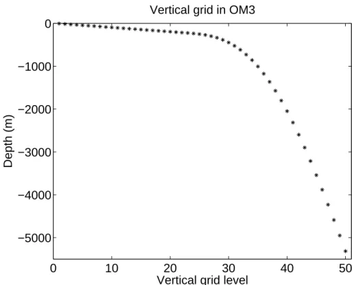
EGU 2.3. Vertical grid resolution

The vertical grid spacing in OM3 was chosen with attention given to the model’s abil-ity to represent the equatorial thermocline as well as processes occuring in the sub-tropical planetary boundary layer. For this purpose, we placed 22 evenly spaced cells in the upper 220 m, and added 28 more cells for the deeper ocean with a bottom at 5

5500 m (see Fig.3).

The representation of solar shortwave penetration into the upper ocean in the pres-ence of chlorophyll (see Sect.2.7) may warrant even finer vertical resolution than that used here (Murtugudde et al.,2002). Other air-sea interaction processes may likewise call for increasingly refined upper ocean resolution. Unfortunately, the use of top grid 10

cells thinner than roughly 10 m can lead to the cells vanishing when run with realistic forcing, especially with pressure loading from sea ice (see discussion inGriffies et al., 2001). Indeed, even with 10 m upper cells, we have found it necessary to limit the overall pressure from sea ice felt by the ocean surface to no more than that applied by 4 m thick ice. Ice thickness greater than 4m is assumed to exert no pressure on the 15

sea surface.

This situation signals a fundamental limitation of free surface methods in z-models. In these models, only the upper grid cell feels motion of the surface height. Refined vertical cells in the presence of a realistically undulating ocean surface height requires alternative vertical coordinates (Griffies et al.,2000a). This issue is a topic of current 20

research and development2.

2.4. Bottom topography and bottom flows

It is common in z-models to have model grid cells at a given discrete level have the same thickness. In these models, it is difficult to resolve weak topographic slopes

with-2

For example, the proposal byAdcroft and Campin(2004) to use the vertical coordinate of

Stacey et al.(1995) for global modelling is of interest given its ability to resolve this problem while maintaining other features familiar to the z-models.

(12)

OSD

2, 165–246, 2005

EGU out including uncommonly fine vertical and horizontal resolution. This limitation can

have important impacts on the model’s ability to represent topographically influenced advective and wave processes. The “partial step” methods ofAdcroft et al.(1997) and Pacanowski and Gnanadesikan(1998) have greatly remedied this problem via the im-plementation of more realistic representations of the solid earth lower boundary. Here, 5

the vertical thickness of a grid cell at a particular discrete level does not need to be the same. This added freedom allows for a smoother, and more realistic, representation of topography by adjusting the bottom grid cell thickness to more faithfully contour the topography. Fig.4illustrates the bottom realized with the OM3 grid along the equator. Also shown is a representation using an older “full step” model with the same horizon-10

tal and vertical resolution. The most visible differences between full step and partial step topography are in regions where the topographic slope is not large, whereas the differences are minor in steeply sloping regions.

The topography used in OM3 was initially derived from a dataset assembled at the Southampton Oceanography Centre for use in their global eddying simulations (An-15

drew Coward, personal communication). This dataset is a blend of several products. Between 72◦S and 72◦N, version 6.2 of the satellite-derived product of Smith and Sandwell (1997) was mapped from the original Mercator projection onto a latitude-longitude grid at a resolution of 2 min. North of 72◦N, a version of the International Bathymetric Chart of the Oceans (Jakobssen et al., 2000) was used, while south of 20

72◦S the ETOPO5 product was used (NOAA,1988).

As mentioned in Sect.2.2, MOM4.0 is a B-grid model in which tracer points are stag-gered relative to velocity points. This grid arrangement necessitates the use of no-slip sidewall conditions for realistic geometries3. Opening channels for advective flow be-tween basins requires the channels to be at least two tracer gridpoints wide. In the 25

presence of complex topography not aligned with the grid, ensuring that basins which are connected in Nature are also connected within the model requires us to dig out

3

Topography tuning must also be combined with viscosity tuning (Sect.3.4) due to the no-slip condition which strongly affects circulation through narrow passages.

(13)

OSD

2, 165–246, 2005

EGU some passages. Significant attention was paid to the North Atlantic overflows

(Den-mark Strait, Iceland-Scotland Overflow, Faeroe Bank Channel) based on the work of Roberts and Wood(1997) suggesting that representation of the sill topography makes important differences in the circulation within the Hadley Centre’s coupled model. Sig-nificant attention was also paid to the topography in the Caribbean Sea as well as the 5

Indonesian Archipelago, where previous work suggests that the exact location of im-portant islands can determine the throughflow in key passages like the Florida, Timor, and Lombok Straits (Wajsowicz,1999). The resulting bottom depth field used in OM3 is shown in Fig.5.

In general, the OM3 bottom topography was arrived at via an extended multi-step 10

process starting originally from the Southampton dataset. Unfortunately, the numerous individual steps were not completely documented, in part because of the use of early versions of the grid generation code that contained errors, and in part because of the hundreds of subjective changes. Additionally, much development work for OM3, including its topography, used a coarser resolution model (the OM2 model). The initial 15

version of the OM3 topography was generated by interpolating the OM2 bathymetry to the finer OM3 grid, and was followed by the subjective modification of hundreds of individual grid depths in an effort to better represent the coastlines and the major bathymetric features (e.g. sills, ridges, straits, basin interconnections) of the World Ocean.

20

Partial steps do not enhance the z-model’s ability to represent, or to parameterize, dense flows near the bottom which often occur in regions where the topographic slope is nontrivial. Indeed, as described byWinton et al. (1998), z-models used for climate rarely resolve the bottom boundary layer present in much of the World Ocean. As a result, dense water flowing from shallow marginal seas into the deeper ocean (e.g. 25

Denmark Strait and Strait of Gibraltar), tend to entrain far more ambient fluid than ob-served in Nature. This spurious entrainment dilutes the dense signals as they enter the larger ocean basins, thus compromising the integrity of simulated deep water masses. As reviewed byBeckmann(1998) andGriffies et al.(2000a), there have been various

(14)

OSD

2, 165–246, 2005

EGU methods proposed to remedy problems simulating overflows in z-models. In OM3, we

implemented the sigma diffusive element of the scheme proposed by Beckmann and D ¨oscher (1997) andD ¨oscher and Beckmann (1999). This scheme enhances downs-lope diffusion within the bottom cells when dense water lies above light water along a topographic slope. Unfortunately, as implemented within the partial step framework, it 5

is possible that the partial steps could become far smaller (minimum 10 m used here) than a typical bottom boundary layer (order 50 m–100 m). In such cases, the diffusive scheme is unable to move a significant amount of dense water downslope through re-gions with thin partial steps. A more promising method is to increase the bottom partial step thickness in regions where overflows are known to be important, or to allow for 10

the sigma diffusion to act within more than just the bottom-most grid cell. We did not pursue either approach for OM3 due to limitations in development time. As a result, the sigma diffusion scheme has a negligible impact on the OM3’s large-scale circula-tion, as evidenced by its very small contribution to the meridional transport of heat (not shown).

15

Although partial steps may be a cause for the insensitivity of the simulation to the sigma diffusion scheme, our results are consistent with those reported by Doney and Hecht (2002), who used the same scheme but in a full step bottom topography model. We are uncertain whether the small impact of the overflow scheme in the coupled model is related to limitations of the overflow scheme algorithm, or to problems with 20

the surface boundary forcing. Hence, although discouraging, we believe these results warrant further focused investigation in process studies and global climate models, es-pecially given the encouraging results from idealized simulations discussed by Beck-mann and D ¨oscher (1997) andD ¨oscher and Beckmann(1999).

2.5. Equation of state 25

Ocean density is fundamental to the computation of both the pressure and physical parameterizations. Hence, an accurate density calculation is required over a wide range of potential temperature, salinity, and pressure. There are two methods we use

(15)

OSD

2, 165–246, 2005

EGU to help make the calculation more accurate in CM2.

Density at a model time step τ is a function of pressure, potential temperature, and salinity at the same time step. However, in a hydrostatic model, pressure is diagnosed only once density is known. Some climate models (e.g.Bryan and Cox,1972) resolve this causality loop by approximating the pressure as p=−ρ_og z, which is the hydrostatic 5

pressure at a depth z<0 for a fluid of uniform density ρ_o. A more accurate method was suggested byGriffies et al.(2001), whereby

ρ(τ)= ρ[θ(τ), s(τ), p(τ − ∆τ)], (1)

with pressure used in the equation of state lagged by a single model time step relative to potential temperature and salinity. As recommended by Dewar et al. (1998), we 10

include contributions from the undulating surface height and loading from the sea ice for the pressure used in the density calculation.

Previous versions of MOM used the cubic polynomial approximation of Bryan and Cox (1972) to fit the UNESCO equation of state documented inGill (1982). This ap-proach has limitations that are no longer acceptable for global climate modelling. For 15

example, the polynomials are fit at discrete depth levels. The use of partial step to-pography makes this approach cumbersome since with partial steps, it is necessary to compute density at arbitrary depths. Additionally, the cubic approximation is inaccurate for many regimes of ocean climate modelling, such as wide ranges in salinity associ-ated with rivers and sea ice. For these two reasons, a more accurate equation of state 20

is desired.

Feistel and Hagen (1995) updated the UNESCO equation of state by using more recent empirical data. In MOM4.0 we utilize a 25 term fit to their work developed by McDougall et al. (2003). The fit is valid for a very wide range of salinity, potential temperature, and pressure that is more than adequate for ocean climate purposes4. 25

4

The McDougall et al. (2003) equation of state is fit over a pressure range from 0 db to 8000 db. The salinity range is 0–40 psu for pressures less than 5500 db, and 30–40 psu for pressures greater than 5500 db. The potential temperature range is freezing to 33◦C for

(16)

pres-OSD

2, 165–246, 2005

EGU 2.6. Tracer advection

As physical climate models evolve to include chemical and biological models appro-priate for the full earth system, they incorporate an increasingly wide array of tracers whose transport is greatly affected by strong spatial gradients in the presence of refined flow features. Many of the earlier compromises with tracer transport are unacceptable 5

with these new model classes. In particular, previous versions of the GFDL ocean cli-mate model used the second order centered tracer advection scheme. Upon recogniz-ing that this scheme is too dispersive, later model versions incorporated the “Quicker” scheme. Quicker is a third order upwind biased scheme based on the work ofLeonard (1979), with Holland et al. (1998) andPacanowski and Griffies (1999) discussing im-10

plementations in ocean climate models. The Quicker scheme is far less dispersive than the second order centered scheme, thus reducing the level of spurious extrema realized in the simulation. However, as with centered differences, problems can occur with unphysical tracer extrema, in particular in regions where rivers enter the ocean thus creating strong salinity gradients. Additional problems can arise with a prognos-15

tic biogeochemistry model, where even slightly negative biological concentrations can lead to strongly unstable biological feedbacks.

There are many advection schemes available which aim to remedy the above prob-lems. Our approach for OM3 employs a scheme ported to MOM4.0 from the MIT GCM5. The scheme is based on a third order upwind biased approach ofHundsdorfer 20

and Trompert (1994) who employ the flux limiters ofSweby(1984). This implementa-tion of numerical advecimplementa-tion is non-dispersive, preserves shapes in three dimensions, and precludes tracer concentrations from moving outside of their natural ranges. The scheme is only modestly more expensive than Quicker, and it does not signficantly al-ter the simulation relative to Quicker in those regions where the flow is well resolved. 25

sures less than 5500 db, and freezing to 12◦C for pressures greater than 5500 db.

5

We thank Alistair Adcroft for assistance with this work. The online documentation of the MIT GCM athttp://mitgcm.orgcontains useful discussions and details about this advection scheme.

(17)

OSD

2, 165–246, 2005

EGU Hence, we have found it to be an essential element of the ocean climate model.

2.7. Penetrative shortwave radiation

The absorption of solar shortwave radiation within the upper ocean varies significantly in both space and time. High levels of chlorophyll result in almost all sunlight being absorbed within just a few meters of the ocean surface in biologically productive waters 5

such as near the equator, in coastal upwelling zones, and polar regions. In contrast, low chlorophyll levels in subtropical gyres allow solar radiation to penetrate with an e-folding depth (in the blue-green part of the visible spectrum) of 20–30 m.

In ocean climate models with thick upper grid cells (e.g. 50 m), the geographic vari-ation of shortwave penetrvari-ation is unimportant since all shortwave radivari-ation is generally 10

absorbed within this single box. In OM3, however, the top box is 10m with a resting ocean free surface. Up to 20% of incoming solar radiation can penetrate below this level in many regions of the ocean. Without allowing shortwave radiation to penetrate, radiative heating would overly heat the top cell, causing its temperature to grow well above observed. One way to address this problem is to allow shortwave penetration 15

with a given e-folding depth that is constant in space and time. However, for long term global climate simulations, we believe it is important to allow geographical and sea-sonal variations of the shortwave penetration. Shy of a prognostic biological model, we choose a climatology rather than a global constant.

Sweeney et al.(2005) compile a seasonal climatology of chlorophyll based on mea-20

surements from the NASA SeaWIFS satellite. They used this data to develop two parameterizations of visible light absorption based on the optical models ofMorel and Antoine (1994) andOhlmann(2003). The two models yield quite similar results when used in global ocean-only simulations, with very small differences in heat transport and overturning. We use theSweeney et al.(2005) chlorophyll climatology in CM2.0 25

and CM2.1 along with the optical model of Morel and Antoine (1994). Although the chlorophyll climatology remains unchanged even when considering changes in radia-tive forcing due to anthropogenic greenhouse gas changes, we believe it is a far better

(18)

OSD

2, 165–246, 2005

EGU means of parameterizing shortwave penetration than available with a global constant

e-folding depth. Future earth system models possessing prognostic biogeochemistry will be better able to represent potential changes in chlorophyll, and hence radiative penetration, under changing climates.

2.8. Background vertical mixing coefficients 5

Vertical tracer diffusion plays a major role in determining the overall structure of the ocean circulation, as well as its impact on climate (Bryan,1987;Park and Bryan,2000). Direct estimates based on measurements of temperature microstructure and the di ffu-sion of passive tracers (Ledwell et al.,1993) indicate that the diffusivity is on the order of 0.1−0.15×10−4m2s−1 in the extra-tropical pycnocline, andGregg et al.(2003) indi-10

cate yet smaller values near the equator. In the deep ocean, both basin-scale budget studies (Whitehead and Worthington, 1982) and direct measurements (Toole et al., 1994, 1997; Polzin et al., 1996, 1997) indicate that diffusivities are on the order of 1−2×10−4m2s−1.

Until recently, most ocean climate models were unable to match the low level of 15

diapycnal diffusivity within the pycnocline suggested from the microstructure and tracer release measurements. The reason they had problems is that some models included high values of spurious diapycnal diffusion associated with the horizontal background diffusion required to stabilize earlier versions of the neutral diffusion scheme (Griffies et al.,1998), and some had large diapycnal diffusion associated with upwind advection 20

(Maier-Reimer et al., 1983). Additionally, earlier GFDL models followed Bryan and Lewis (1979) and used a vertical diffusivity of 0.3×10−4m2s−1 in the upper ocean and 1.3×10−4m2s−1 in the deep ocean. Higher levels of vertical diffusion within the thermocline result in an increase in tropical upwelling and poleward heat transport in both hemispheres (Gnanadesikan et al.,2003) which may compensate for the relative 25

sluggishness of boundary currents in the coarse models.

In OM3, we maintain a relatively refined vertical resolution in the upper ocean, largely to allow for a realistically small vertical diffusivity within the tropical thermocline.

(19)

Mod-OSD

2, 165–246, 2005

EGU elling experience indicates a strong sensitivity of the equatorial current structure and

ENSO variability to the levels of tracer diffusion, with realistic simulations requiring small values consistent with the observations (Meehl et al.,2001).

Simmons et al. (2004) illustrate the utility of including a parameterization of mixing associated with breaking internal waves arising from the conversion of barotropic to 5

baroclinic tidal energy. Such wave breaking occurs especially above regions of rough bottom topography (Polzin et al., 1997). The results from the Simmons et al. (2004) simulations indicate that a small value through the pycnocline and larger value at depth, qualitatively similar to the profile ofBryan and Lewis(1979), is far better than a vertically constant diffusivity.

10

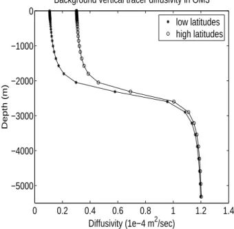
While the Simmons et al. (2004) work remains the subject of much research, we decided to maintain the approach ofBryan and Lewis(1979) by prescribing a flow in-dependent background diffusivity for OM3. To reflect the observations noted above, we modified the canonical Bryan and Lewis (1979) values to the smaller levels of 0.1×10−4m2s−1 in the upper ocean and 1.2×10−4m2s−1 in the deeper ocean within 15

the tropics. In the high latitudes, although not suggested from observations, we used the larger value of 0.3×10−4m2s−1 in the upper ocean. Figure7 shows the vertical profile of background vertical tracer diffusivity.

Figure 8 shows effects on the North Atlantic sea surface salinity (SSS) in CM2.0 arising from increased Bryan-Lewis vertical diffusivity in the high latitudes. Increased 20

mixing reduced the global rms error in the coupled model from 0.84 to 0.79, and in the North Atlantic from 1.57 to 1.41. The main goal of the increased tracer diffusion in the high latitudes was not necessarily to reduce the SSS biases by this modest level. Rather, it was to address a model bias in the subpolar North Atlantic towards weak Labrador Sea deepwater formation, and a perceived fragility of simulated Atlantic 25

overturning. In retrospect, this ocean bias was largely associated with the equatorial shift of the wind stress in the atmospheric model discussed in Sect. 1.3 and more fully in Delworth et al. (2005). Consequently, the enhanced vertical tracer diffusivity likely was unneeded in CM2.1 where the finite volume atmospheric model does not

(20)

OSD

2, 165–246, 2005

EGU have an equatorial bias. Indeed, the overturning circulation is quite vigorous in CM2.1

(Delworth et al.,2005). Limitations in resources and time precluded our re-tuning the vertical diffusivity in CM2.1.

Many modelers have traditionally taken a Prandtl number (ratio of viscosity to di ffu-sivity) on the order 1–10. In OM3, we choose a depth independent background vertical 5

viscosity of 10−4m2s−1. The level of background viscosity can also affect the equatorial currents, as discussed inLarge et al.(2001). There is no theoretical or observational justification for this value of the vertical viscosity.

2.9. Surface ocean boundary layer

In addition to the background vertical diffusivity and viscosity discussed in Sect. 2.8, 10

we use the parameterization of boundary layer mixing proposed byLarge et al.(1994). This k-profile parameterization (KPP) scheme prescribes added levels of tracer and velocity mixing in regions where mixing is likely to be under-represented in this hydro-static model, such as in the important surface ocean boundary layer. The KPP scheme has been used by many climate models during the past decade. It provides a suitable 15

framework within which to consider various mixing processes.

Beyond the standard settings recommended byLarge et al. (1994), interior mixing in OM3 is enhanced by double diffusion due to salt fingering and diffusive convection. These processes occur in regions where the vertical temperature and salinity gradients have the same sign, and so contribute oppositely to the vertical density gradient (see 20

Schmitt, 1994; Toole and McDougall, 2001; Kantha and Clayson, 2000, for reviews of these processes). Additionally, the Richardson number computation is modified by adding to the resolved vertical shear an unresolved shear due to tidal velocities diagnosed from a tide model according to the methods discussed inLee et al.(2005). These tidal velocities are significant near coastal regions (see Fig.9), in which case 25

the Richardson numbers are small thus enhancing the vertical mixing coefficients. We found this extra mixing to be especially useful in certain river mouths to assist in the

(21)

OSD

2, 165–246, 2005

EGU horizontal spreading of river water into the ocean basins by the horizontal currents.

3. Novel methods and some lessons learned

The purpose of this section is to highlight numerical and physical features of the ocean climate model that are either novel or where novel insights and experiences were gar-nered.

5

3.1. Ocean free surface and freshwater forcing

Variations in the ocean free surface are precluded in models using the rigid lid approx-imation ofBryan (1969a). This approximation was commonly made in early climate models for computational expendiency since it filters out fast barotropic undulations of the ocean free surface. However, as noted byGriffies et al. (2001), rigid lid models 10

exhibit poor computational efficiency on parallel computers. The reason is that the elliptic problem associated with the rigid lid involves global communication across all parallel computer processors. This type of communication is costly on machines us-ing a distributed computer processor architecture (i.e. the machines typically used for global climate modelling). Explicit free surface methods only involve less costly local 15

processor communication, which generally leads to a far more efficient algorithm. There are physical consequences that must be considered when making the rigid lid approximation. First, the rigid lid distorts the dispersion relation for planetary waves, especially those waves with spatial scales on the order of the barotropic Rossby ra-dius (thousands of kilometers). Second, as commonly implemented in ocean climate 20

models, the rigid lid precludes the transport of water across ocean boundaries. The reason is that the volume of all grid cells is fixed in time, thus precluding transport of water across ocean boundaries. Hence, there is no barotropic advection giving rise to the Goldsborough-Stommel circulation, and freshwater dilution of tracer concentrations must be parameterized (seeHuang,1993;Griffies et al.,2001, and references therein 25

(22)

OSD

2, 165–246, 2005

EGU for more thorough discussion of these issues).

The ocean’s density, and hence its pressure and circulation, are strongly affected by the transport of water across the ocean boundaries via evaporation, precipitation, river runoff, and ice melt. That is, ocean boundaries are open to water fluxes, and these fluxes are critical to ocean dynamics. Additional climatologically important tracers, such 5

as dissolved inorganic carbon, are also affected by water transport, as is the ocean’s alkalinity. “Virtual salt fluxes” used in fixed volume ocean models aim to parameterize the effects of boundary water transport on the density field. Such models transport salt, rather than water, across the air-sea interface. However, only a neglible amount of salt crosses Nature’s air-sea interface. Additional virtual fluxes are required in constant 10

volume models for other tracers. In general, virtual tracer flux methods can distort tracer changes, such as in the climatologically important situation discussed below where salinity is low as near river mouths.

Free surface methods, such as the one proposed byGriffies et al.(2001) andGriffies (2004) render the ocean volume time dependent. A time dependent ocean volume 15

opens ocean boundaries so that water can be exchanged with other parts of the cli-mate system. Such water transport across boundaries manifests as changes in ocean surface height (see equation (32)). When formulated in this way, virtual tracer fluxes are inappropriate. Free surface methods also remove the distortion of barotropic planetary waves since they allow for time dependent undulations of the ocean’s free surface. 20

Although most ocean climate models today employ a free surface, tracer budgets in many models still assume the ocean volume is constant. That is, they do not allow water to be exchanged with other parts of the climate system. We therefore find it in-teresting to consider how the response of salinity to a freshwater perturbation differs in a model that uses virtual tracer fluxes from a model allowing water to cross its bound-25

aries. For this purpose, consider an ocean comprised of a single grid cell affected only by surface freshwater fluxes. Conservation of salt in a Boussinesq model leads to

∂_t(h s)= 0 (2)

(23)

OSD

2, 165–246, 2005

EGU can change, the thickness of the ocean is altered by the addition of freshwater via

∂_th= q_w (3)

where q_w=P −E+R+I is the volume per horizontal area per time of precipitation, evapo-ration, river runoff, and ice melt that crosses the ocean surface (Eq.25in the appendix). In this case, salinity evolves according to

5

h ∂_ts= −s q_w. (4)

For example, freshwater input to the ocean (q_w>0) dilutes the salt concentration and so reduces salinity.

In a model using a fixed volume, salinity evolves according to

h ∂_ts= −srefq_w, (5)

10

where now h is time independent, and s_refis a constant salinity needed to ensure that total salt is conserved in the constant volume model assuming fresh water is balanced over the globe6. The virtual salt flux is given by

F(virtual salt) = srefq_w. (6)

Models have traditionally taken sref=35, as this is close to the global averaged salinity 15

in the World Ocean.

Use of a global constant normalization distinguishes the salinity budget (Eq. 5) in the virtual salt flux model from the local salinity used in a model that exchanges water with its surroundings (Eq. 4). To illustrate how this factor alters the salinity response to freshwater forcing, consider a case where fresh river water is added to a relatively 20

6

Total salt is not conserved in constant volume models using the salinity Eq. (4) appropriate for real freshwater flux models. Nonetheless, attempts have been made at GFDL to run con-stant volume models with the salinity Eq. (4) in an aim to properly simulate the local feedbacks on salinity from freshwater. Unfortunately, such models tend to have unacceptably large drifts in salt content and so have not been used at GFDL for climate purposes.

(24)

OSD

2, 165–246, 2005

EGU fresh ocean region where s<s_ref (e.g. rivers discharging into the Arctic Ocean). Here,

since the actual local salinity is fresher than the globally constant reference salinity, the dilution effect in the virtual salt flux model will be stronger than the real water flux model. Such overly strong feedbacks can introduce numerical difficulties (e.g. advection noise and/or salinity going outside the range allowable by the equation of 5

state) due to unphysically strong vertical salinity gradients. For OM3, we have found problems with overly fresh waters to be particularly egregious in shallow shelf areas of the Siberian Arctic. For the opposite case where evaporation occurs over salty regions with s>s_ref (e.g. evaporation over subtropical gyres), the virtual salt flux model under-estimates the feedbacks onto salinity.

10

We now illustrate how the use of virtual salt fluxes alter the simulation characteristics in the coupled climate model relative to real water fluxes. For this purpose, we ran two CM2.1-like climate models for a short period of time. In the standard CM2 experiments, water is input as a real water flux that affects the surface height by adding volume to the ocean fluid. For the purpose of comparison with a virtual salt flux run, we insert river 15

water just into the top model grid cell7. We ran a second experiment with virtual salt fluxes where the virtual salt fluxes associated with the river water are applied over the top cell. Consistent with the previous theoretical discussion, results in Fig.10, taken in August of the second year, show that the virtual salt flux model has systematically fresher water near river mouths, with largest differences around 14 psu fresher. Away 20

from rivers, the differences are minor, and consistent with variability. The virtual salt flux experiment became numerically unstable in October of the second year due to extremely unphysical values of the salinity, whereas the real water flux experiment remained stable.

In conclusion, virtual tracer fluxes can do a reasonable job of parameterizing the 25

effects of freshwater on tracer concentration in regions where the globally constant ref-erence tracer concentration is close to the local concentration. However, for realistic

7

In the standard CM2 experiments, river water is inserted throughout the upper 40m of the water column in a manner described in Sect.3.6.

(25)

OSD

2, 165–246, 2005

EGU global climate models, local concentrations can deviate significantly from the global

ref-erence, especially near river mouths. This deviation compromises the physical realism and numerical stability of the simulation. These are the key reasons that we jettisoned virtual tracer fluxes in our standard climate model simulations in favor of allowing water fluxes to cross the ocean model boundaries8.

5

3.2. Time stepping the model equations

As noted by Griffies et al. (2000a), the leap frog remains the most commonly used method for discretizing the time tendency in primitive equation ocean climate models. OM3.0 retains this approach. However, an alternative time stepping scheme was de-veloped for OM3.1. This time staggered method has much in common with that used 10

in HIM (Hallberg,1997) as well as the MIT GCM (Marshall et al.,1997;Campin et al., 2004). Details of the scheme are provided in Chapter 12 of Griffies (2004). We in-troduce the main features here since the scheme possesses some highly favorable characteristics of use for ocean climate modelling. We also illustrate sensitivity of the simulation to the time stepping algorithm by comparing model integrations with the leap 15

frog to the time staggered scheme.

3.2.1. Characteristics of staggered time stepping

Leap frog tendencies lead to time splitting which necessitates the use of time filter-ing (e.g.Haltiner and Williams,1980;Durran,1999). Filters reduce the second order accurate leap frog to first order (Durran, 1999). Additionally, when realized with an 20

undulating free surface as in OM3,Griffies et al.(2001) showed how time filters make it nontrivial to satisfy the constraints of both local and global tracer conservation. Lo-cal conservation means that a uniform tracer concentration remains unchanged in the

8

The impact of virtual salt fluxes on forcing of the meridional overturning circulation in the North Atlantic is currently under investigation by researchers at GFDL (Ron Stouffer, personal communication).

(26)

OSD

2, 165–246, 2005

EGU absence of boundary tracer fluxes even in the presence of momentum fluxes. Global

conservation means that boundary tracer fluxes are precisely balanced by changes in tracer content in the full model domain. Both forms of conservation are important for earth system modelling.

The new scheme discretizes time tendencies with a forward time step. Second order 5

accuracy is maintained by staggering tracer and velocity fields by one-half time step in a manner analogous to spatial staggering on Arakawa grids. We therefore refer to this method as a staggered scheme9. As forward time stepping schemes do not admit time splitting modes, no time splitting mode exists, and so no time filters are needed. The new scheme therefore ensures both local and global tracer conservation.

10

Temporal stability of the staggered scheme is twice that of the leap frog in cases where the model’s time step is constrained by either gravity waves or dissipation. To understand this very important practical result, recall that the leap frog updates the ocean state by a∆τ time step, yet it employs 2∆τ for the tendency calculation. Hence, gravity waves and dissipative operators (i.e. diffusion, friction, and upwind biased ad-15

vection) have stability properties based on 2∆τ. The staggered scheme updates the ocean state by∆τ and it employs ∆τ to compute tendencies. Hence, its stability prop-erties are based on the∆τ time step.

Preliminary analysis of the leap frog version OM3.0 reveals that its time step is largely constrained by friction along the equatorial region within the western boundaries, espe-20

cially in the Indonesian region. Hence, the above stability result indicates that OM3.1 should be stable with twice the time step using the staggered scheme as required for the leap frog. Indeed, this is the case. That is, when OM3.0 is stable with the leap frog scheme using a time step∆τleap, OM3.1 has been found to be stable using the

9_{We retain second order centered differencing for the velocity advection, thus prompting the}

use of an Adams-Bashforth method to time discretize this term (Durran,1999). We chose the temporally third order accurate scheme for this purpose due to its enhanced stability properties over the second order scheme.

(27)

OSD

2, 165–246, 2005

EGU staggered scheme with twice the time step

∆τstag= 2∆τleap. (7)

Consequently, the computational cost of OM3.1 with the staggered scheme is one-half that of OM3.0 which uses the leap frog scheme.

To illustrate the time staggered method, it is sufficient to consider an update of thick-5

ness weighted tracer (see Sect.19for discussion of the tracer equation). With a leap frog discretization of the time tendency, we compute

(h T )τ+∆τleap − (h T )τ−∆τleap

2∆τleap =

−∇ · [ (h u)τ_Tτ−_∆τleap_{+ h}τ_Fτ−_∆τleap

] − δ_k[ wτTτ−∆τleap+ F_zτ+∆τleap], (8) where h and T are the time filtered values of the tracer cell thickness and concentration, 10

(u, w) are the advection velocity components, (F, F_z) are the SGS fluxes, ∇ is the hor-izontal gradient operator, and δ_k is the vertical finite difference operator. Note that the vertical SGS flux component F_z is evaluated implicitly in time, and the advective fluxes are computed assuming an upwind biased scheme so that the tracer concentration is lagged in time just as the horizontal SGS flux (e.g.Holland et al.,1998;Pacanowski 15

and Griffies, 1999). The time time staggered form of the discrete tracer equation is given by (h T )τ+12∆τstag− (h T )τ− 1 2∆τstag ∆τstag = −∇ · [ (h u)τ_Tτ−1 2∆τstag+ hτFτ− 1 2∆τstag] − δ k[ wτT τ−1_2∆τstag + Fτ+12∆τstag z ]. (9)

Except for the time filtering applied to the leap frog method, the two Eqs. (8) and (9) are 20

identical when∆τstag=2∆τleap. However, no time steps are skipped when computing discrete time tendencies with the time staggered method, since this approach employs

(28)

OSD

2, 165–246, 2005

EGU forward time differences. No time filtering is therefore needed in this approach. In

effect, the time staggered method stays on just one of the two leap frog branches. This is the fundamental reason that the staggered method should be expected, for many purposes, to yield similar solutions to the leap frog yet at half the computational cost. 3.2.2. Implicit and semi-implicit terms

5

As with many other ocean climate models, we time step the vertical physical processes (i.e. vertical diffusion and vertical friction) with an implicit time step. In the staggered method, the implicit portion leads the explicit portion by a single time step, whereas the implicit leads by two time steps with the leap frog. The staggered scheme is thus more accurate for the vertical implicit processes.

10

In the velocity equation, we implement the Coriolis force semi-implicitly (Eq.21). This method is second order accurate, which is shared by a time explicit implemention. We prefer the semi-implicit method as it provides some added stability in practice. Although the model’s baroclinic time step is well within the range needed to resolve inertial os-cillations, extra stability is useful to suppress an inertial instability of the coupled ocean 15

and sea ice system10. Note that inertial energy is quite strong in the coupled model since the atmosphere and land models have a diurnal cycle whereby the atmospheric and sea ice fields felt by the ocean (stress, fresh water, turbulent and radiative fluxes) are updated every 3 h11. Inertial energy has important contributions to the mixing co-efficients determined by the model’s boundary layer scheme (Sect.2.9).

20

3.2.3. Sensitivity to the time stepping scheme

During the bulk of our development process, the ocean model employed the leap frog scheme for the tracer, baroclinic, and barotropic equations. However, upon

develop-10

The precise mechanism of this instability is under investigation.

11

As recommended byPacanowski(1987), wind stress applied to the ocean surface is com-puted using the relative velocity between the atmospheric winds and the ocean currents.

(29)

OSD

2, 165–246, 2005

EGU ing the staggered time stepping scheme for the tracer and baroclinic equations, and

a predictor-corrector for the barotropic equations (Killworth et al.,1991), we became readily convinced that the new time stepping schemes were better from both funda-mental numerical and practical model efficiency perspectives. The question arose whether switching to the new time stepping schemes would require retuning of the 5

physical parameterizations.

Preliminary tests were run with the ocean and ice models using an annually repeat-ing atmospheric forcrepeat-ing with daily synoptic variability, again repeatrepeat-ing annually. Runs using the new time staggered scheme had a 2 h time step for both tracer and baro-clinic momentum, and a predictor-corrector scheme (e.g.Killworth et al.,1991;Griffies, 10

2004) for the barotropic equations with a 90 s time step. We prefer the predictor-corrector for the barotropic equations due to its increased stability relative to the leap frog, as well as its ability to dissipate grid scale noise commonly found when simulating gravity waves on a B-grid (Killworth et al.,1991; Griffies et al.,2001). The compari-son was made to a leap frog ocean using 1 h time steps for the tracer and baroclinic 15

equations, and (3600/64) s for the leap frog barotropic equations.

Analysis of these solutions after 10 years revealed that regions with high frequency temporal variability, such as the equatorial wave guide, exhibit the most differences in-stantanously. Figure11 illustrates the situation along the equator in the East Pacific. The leap frog simulation exhibits substantial splitting behaviour, even with a nontrivial 20

level of time filtering from a Robert-Asselin filter (Haltiner and Williams,1980;Durran, 1999) aiming to suppress the splitting. Moving just 5◦N of the equator, however, reveals that the simulation has much less relative variability, and a correspondingly negligible amount of time splitting. Even though the simulation along the equator showed sub-stantial time splitting, over time the large scale patterns and annual cycles showed 25

negligible differences between time stepping schemes. Time averaging, even over just a day, seems sufficient to smooth over most of the instantaneous differences.

Tests were then run with CM2.0 and CM2.1. Instantaneous differences were much larger, as expected due to the nontrivial natural variability in the coupled system with

(30)

OSD

2, 165–246, 2005

EGU a freely evolving atmosphere. Nonetheless, differences for large scale patterns and

seasonal or longer time averages were within levels expected from the model’s natural variability.

Differences do occur due to (1) different barotropic time schemes, (2) third or-der Adams-Bashforth for momentum advection, (3) differences in implicit physics, (4) 5

Robert-Asselin filtering in the leap frog scheme. But to the extent that the solution is dominated by geostrophically balanced flow, the time stepping schemes should pro-duce similar results. It is pleasantly surprising that the solutions maintain close corre-spondence even in the equatorial region and in regions of strong deep convection.

Although our tests revealed only minor differences between the two time stepping 10

schemes, we believe the analysis and results in this section provide compelling reasons to eschew leap frog time schemes for ocean climate modelling. Troubles realizing tracer conservation create difficulty when integrating for centuries, or when developing new component models such as biogeochemical or ecosystem models. We conjecture that the small differences noted in our tests will accumulate on the centennial and 15

longer time scales, although we are not prepared to run the coupled model to rigorously test the level to which the solutions drift apart.

3.2.4. Comments on time stepping schemes

In general, the leap frog time splitting mode is very unsatisfying from a fundamental numerical perspective. Furthermore, the practical bottomline is that the conservative 20

staggered scheme is about twice as stable as the leap frog scheme. These conclusions are likely unsurprising to those familiar with the computational fluid dynamics literature (e.g.Durran,1999), where leap frog methods have long since been abandoned. How-ever, as documented byGriffies et al.(2000a), the majority of ocean climate models still use the leap frog, with the notable exception ofHallberg(1997),Marshall et al.(1997), 25

and Campin et al. (2004). We believe the GFDL model documented in this paper is the only model contributing to the Fourth IPCC assessment that does not use a leap frog based method. As shown here, alternative methods can provide a straightforward