Analysis of water vapor LIDAR measurements during the MAP campaign: evidence of sub-structures of stratospheric intrusions

(1)

HAL Id: hal-00301565

https://hal.archives-ouvertes.fr/hal-00301565

Submitted on 15 Dec 2004

HAL is a multi-disciplinary open access

archive for the deposit and dissemination of sci-entific research documents, whether they are pub-lished or not. The documents may come from teaching and research institutions in France or abroad, or from public or private research centers.

L’archive ouverte pluridisciplinaire HAL, est destinée au dépôt et à la diffusion de documents scientifiques de niveau recherche, publiés ou non, émanant des établissements d’enseignement et de recherche français ou étrangers, des laboratoires publics ou privés.

Analysis of water vapor LIDAR measurements during

the MAP campaign: evidence of sub-structures of

stratospheric intrusions

P. d’Aulerio, F. Fierli, F. Congeduti, G. Redaelli

To cite this version:

P. d’Aulerio, F. Fierli, F. Congeduti, G. Redaelli. Analysis of water vapor LIDAR measurements during the MAP campaign: evidence of sub-structures of stratospheric intrusions. Atmospheric Chemistry and Physics Discussions, European Geosciences Union, 2004, 4 (6), pp.8327-8355. �hal-00301565�

(2)

ACPD

4, 8327–8355, 2004

Water vapor LIDAR measurements during stratospheric intrusions P. D’Aulerio et al. Title Page Abstract Introduction Conclusions References Tables Figures J I J I Back Close Full Screen / Esc

Print Version Interactive Discussion

Atmos. Chem. Phys. Discuss., 4, 8327–8355, 2004 www.atmos-chem-phys.org/acpd/4/8327/

SRef-ID: 1680-7375/acpd/2004-4-8327 European Geosciences Union

Atmospheric Chemistry and Physics Discussions

Analysis of water vapor LIDAR

measurements during the MAP campaign:

evidence of sub-structures of

stratospheric intrusions

P. D’Aulerio1, 2, F. Fierli1, F. Congeduti1, and G. Redaelli2

1

Institute of Atmospheric Sciences and Climate, CNR, Roma, Italy

2

Department of Physics, University of L’Aquila, L’Aquila, Italy

Received: 17 August 2004 – Accepted: 16 November 2004 – Published: 15 December 2004 Correspondence to: P. D’Aulerio (p.daulerio@isac.cnr.it)

(3)

ACPD

4, 8327–8355, 2004

EGU

Abstract

This paper presents case studies of dehydration in the free troposphere measured by a ground based Raman LIDAR in the Northern-Italy, during the Mesoscale Alpine Pro-gramme (MAP). Two observations characterized by the presence of anomalously dry layers, below 6 km height, were analyzed using Lagrangian techniques. These events 5

are related to upper-tropospheric, high Potential Vorticity streamers crossing the Alpine region and are interpreted as small-scale features of stratospheric intrusions associ-ated to the PV ridge during its breakout phase. One of the measurements also shows the presence of two distinct dehydrated structures associated to the same event. The water vapor concentration also suggests dilution processes of dry stratospheric air in 10

the troposphere. Lagrangian simulations allowed to successfully reproduce the ob-served water vapor distribution and the air parcel histories confirmed the stratospheric origin of the dry layers.

1. Introduction

The transfer of stratospheric air in the troposphere is considered among the key mecha-15

nisms influencing the short term variability of the water vapor distribution in the upper-troposphere (SPARC, 2000). Evidence indicates that Stratosphere-Troposphere ex-changes (STEs) are also the most important natural factor to impact the tropospheric ozone budget; therefore, due to the radiative properties of ozone and water vapor, these mechanisms can have a strong bearing on the radiative balance. Moreover, the 20

intrusions of PV-rich and dry air in the troposphere can affect some aspects of tropo-spheric dynamics (e.g. Vaughan and Worthington, 2000, and references therein).

Stratospheric intrusions at middle latitudes are mainly associated to tropopause folds (Danielsen, 1968) and can be observed at the synoptic scale as streamers of dry air on satellite images (Appenzeller and Davies, 1992) or anomalies of Potential Vorticity 25

(4)

ACPD

4, 8327–8355, 2004

in ozone, water vapor and PV between stratospheric and tropospheric air (Appenzeller et al., 1996). A higher resolution of the streamers within the synoptic representation is achieved by comparing the specific humidity to the corresponding PV, as shown by Gray et al. (1994) and Cox et al. (1995).

Stratospheric intrusion events are not always representative of an effective exchange 5

between the stratosphere and troposphere. In fact, irreversible transport depends on the degree of fragmentation in the finer structures of the air transported from the strato-sphere down into the tropostrato-sphere (Vaughan et al., 1994; Appenzeller et al., 1996; Langford and Reid, 1998). As a result of the filamentation, laminar distributions along the vertical profiles of the transported chemical species appear with respect to the 10

climatological profiles (Newell et al., 1999), with a rapidly decreasing vertical depth versus time (Methven et al., 2003). This effect can persist in the atmosphere several days later than the intrusion in the troposphere (Bithell et al., 2000). The irreversible mixing of stratospheric and tropospheric air during the lifetime of the folding, is influ-enced by different mechanisms such as radiative processes, turbulence and molecular 15

diffusion (Shapiro, 1980; Appenzeller et al., 1996; Forster and Wirth, 2000).

The impact of such episodes in the quantitative cross-tropopause flux and a com-plete definition of mechanisms responsible for irreversible mixing can be still considered crucial aspects for an appropriate description of STE in the extratropics, as summarized in the review paper of Stohl et al. (2003).

20

The observations of deep intrusion episodes, along with their reproduction in numer-ical models, represent an important requirement for such purposes. In fact, it has been shown that the occurrence of deep intrusions in the lowermost troposphere can impact the efficiency of the exchange, favoring irreversible transport (Eisele et al., 1999).

LIDAR presented itself as an appropriate tool to resolve the spatial scale of the struc-25

tures associated with the folding and to provide information about the evolution of such small scale features. This is due to the high spatial and temporal resolution of data and the capability of a continuous sounding (over several hours) of ozone and water vapor profiles (Ancellet et al., 1991; Langford and Reid, 1998; Eisele et al., 1999; Ravetta

(5)

ACPD

4, 8327–8355, 2004

EGU

and Ancellet, 2000; Bertin et al., 2001).

This paper presents the analysis of tropospheric water vapour measurements from a ground-based LIDAR during the MAP-SOP (Mesoscale Alpine Programme - Special Observing Period) campaign. The use of water vapour as a tracer of stratospheric in-trusions allows for the clear identification of small-scale (<1 km thick) dry structures as 5

filaments originating from the stratosphere. These filaments penetrate into the lower troposphere (down to 3000 m) and persist for at least 48 h after their intrusion. In the first part of the paper the measurement technique, the error budget assessment and the modeling tools are presented. The second part of the paper is devoted to the anal-ysis of two case studies, focusing on a quantitative comparison between simulations 10

and the measured water vapor profiles and on the identification of the origin of the observed dry air by using Lagrangian techniques.

2. Measurements

A RMR (Rayleigh/Mie/Raman) LIDAR was deployed during the MAP-SOP in Pal-lanza di Verbania (45.9◦N–8.5◦E, 200 m a.s.l.), inside the “Lago Maggiore Target Area” 15

(Northern Italy). The main purpose of the MAP program was the study of extreme events influenced by orography and the improvement of complex topography effect within numerical models (Bougeault et al., 2002). In this framework, the study of the role of upper-tropospheric PV anomalies on the alpine meteorology was a main task, requiring the investigation of the fine-scale structures and their influence on at-20

mospheric processes in the alpine region. In fact, interactions of PV anomalies with orography has been indicated as an element affecting meteorological events such as cyclogenesis and precipitation on the Alpine lee side (Massacand et al., 1998; Liniger and Davies, 2003).

The LIDAR, developed at ISAC-CNR (Institute of Atmospheric Sciences and Climate 25

– National Research Council), is schematically composed of a transmitter sending two-laser beams vertically into the atmosphere, at wavelength of 532 nm and 355 nm

(6)

(sec-ACPD

4, 8327–8355, 2004

ond and third harmonics of an Nd:YAG pulsed laser) and of a multichannel receiver. The experimental configuration was designed for retrieving water vapor, temperature and aerosols with maximum accuracy in the widest atmospheric range. The basic res-olution of acquisitions is 1 min in time and 75 m in altitude using photocounting (Con-geduti et al., 2002). The water vapor profiles, in mixing ratio units, are determined by 5

inverting the ratio of the signal corresponding to the 355 nm-Raman shifted radiation that is backscattered by H₂O and N₂atmospheric molecules.

This ratio is proportional to water vapor concentration, since the molecular nitrogen can be assumed to have constant mixing ratio within the altitude range of measure-ments. In order to retrieve the water vapor in mixing ratio units, it is necessary to 10

estimate a constant, depending on the instrumental characteristics, by comparison with an independently measured water vapor profile. The detailed inversion procedure is described in literature (e.g. Whiteman et al., 1992). For each single measurement session, the LIDAR profiles have been compared with high-resolution radiosoundings launched at Milano Linate Airport, 75 km southeast of the LIDAR site, in the proximity 15

of a large urban area and inside the Po valley. The comparison shows generally a good agreement between the instruments in the free troposphere, particularly in absence of strong horizontal motion. As expected, significant differences are found in the PBL where the water vapor distribution is strongly related to local conditions. For this rea-son, the calibration procedure is always performed at an altitude above 2000 m. The 20

radiosonde-LIDAR comparison also allowed for an upper estimation of the systematic error introduced by the calibration method of 10%. On average, the statistical uncer-tainty is less then 10% up to the middle troposphere, increasing up to more than 40% in the upper troposphere (>9 km–10 km), for an integration time of 30 min. The signal to noise ratio also depends on the absolute moisture concentration, for example in dry 25

conditions higher values for the statistical error are expected. Generally, the water va-por data acquired during the campaign by the Raman LIDAR are available from few hundred meters above the ground up to a maximum altitude of 10–10.5 km. During the campaign, 26 nighttime LIDAR measurements were carried out for a total of 160 h

(7)

ACPD

4, 8327–8355, 2004

EGU

of observations. Two observations during tropopause folding episodes detected above the Alpine region were identified and analyzed in the following part of the paper.

3. Lagrangian simulations

To interpret LIDAR observations, Lagrangian simulations from the trajectory model FLEXTRA (Stohl, 1998) have been performed. The model uses the analysis of the 5

European Centre for Medium-Range Weather Forecasts (ECMWF) operational global assimilation schemes at a 3 h temporal resolution, 0.5◦×0.5◦horizontal resolution and 60 vertical levels (T312 truncation).

The lagrangian approach is based on the calculation of “Coherent Ensemble of Tra-jectories” (CETs) identified as groups of trajectories showing a marked coherency with 10

the time and obtained by computation from a large number of fixed grid-points. There-fore, the mean properties of each group along the path can be statistically estimated. This method is shown to be appropriate in the analysis of sub-synoptic systems in the study of extratropical cyclones and cross-tropopause exchanges (Wernli and Davies, 1997). In the present study, 3-D and isentropic CET have been calculated in a domain 15

including the LIDAR position in order to identify the origin of the measured air parcels with a better statistical significance of the results with respect to the calculation on the single grid point. For this, a regular grid is defined around the LIDAR site and the air parcels are advected backward in time at each grid point. The backward time-length of simulations ranges between 48–96 h, depending on the numerical dispersion of the 20

trajectory cluster.

The 3-D grid is defined in a spatial range between 42◦N and 50◦N in latitude and 4.5◦E and 12.5◦E in longitude, with an horizontal path equal to the ECMWF data (i.e. 0.5◦), for an altitude range between 3 and 8 km, every 250 m. CETs are also calculated in a limited sub-grid. The 3-D trajectories provided more accurate reproduction of the 25

observed characteristics and therefore only the results of 3-D simulations are shown in this context.

(8)

ACPD

4, 8327–8355, 2004

The back-trajectories are also used to perform a Lagrangian Tracer Reconstruction (LTR) based on the Reverse Domain Filling (RDF) technique. This is to reproduce high resolution water vapor and PV fields during the observation period; these fields can be directly compared to the measured water vapor distribution.

The RDF technique, originally proposed by Sutton et al. (1994), has been extensively 5

employed in studies concerning the dynamic of the polar vortex and the interpretation of laminae measured in stratospheric ozone profiles (Orsolini et al., 1998; Manney et al., 1998; Dragani et al., 2002). This approach has been also used in the simulation of tropospheric moisture (Pierrehumbert, 1998) and ozone and water vapor distributions in the upper troposphere (Methven et al., 2003).

10

This method amplifies the gradients in the physical parameters, not resolved by con-ventional meteorological analysis. In fact, if neighboring parcels have a different origin, their back-trajectories spread out with increasing of simulation time.

A simplified variant of this technique has been applied for LTR imposing the specific humidity concentration and PV, experienced by the air parcels along the back-trajectory 15

at a defined time τ, to each grid point. This allows the reconstruction of the 3-D tracer field surrounding the observation site as a function of time. The time length τ, is limited by the condition for water vapor and PV conservation. In fact, while in the stratosphere water vapor and PV can be assumed to be conserved for 10–15 days on an isentropic surface (Knudsen and Carver, 1994), the tropospheric water vapor is characterized by 20

a lower conservation time scale, affected by condensation phenomena and diabatic motion. Moreover, trajectory dispersion can lead, in some cases, to an unrealistic field reconstruction. In this case, values of τ ranging between 12–24 h have been chosen in order to optimize the agreement with the LIDAR measurements.

The comparison between the LTR water vapor fields and LIDAR data, indicates that 25

condensation along the trajectories can lead to an overestimate of the water vapor content (Methven et al., 2003). In order to avoid this effect, the advection is performed backward until reaching saturation conditions when the “memory” of previous water vapor content along the trajectory has been lost (Pierrehumbert, 1998). The

(9)

recon-ACPD

4, 8327–8355, 2004

EGU

structed mixing ratio was then assumed equal to the minimum value of saturation mix-ing ratio within the chosen interval, under the realistic hypothesis to be outside of a region characterized by relevant sources of moisture. By this procedure the humidity excess is rather well eliminated if compared with the observations.

4. 7 November 1999 case study during the MAP IOP 15

5

A PV anomaly, developed in the Western Atlantic and experiencing a southeastward motion, crossed the Alpine region between 5 and 8 November 1999. The MAP IOP 15 (Intensive Observing Period) was dedicated to the study of this event (Bougeault et al., 2002; Hoinka et al., 2003; Liniger and Davies, 2003). The early and central phase of the streamer evolution was characterized by strong rain conditions associated with 10

the orographic cyclone that developed on the alpine lee-side (Buzzi et al., 2003). This allowed for LIDAR observations only after 7 November at 06:00 p.m. until 04:00 a.m. of the following day, when the streamer is found in its breaking phase, as seen in the simultaneous synoptic PV maps (not reported).

Hoinka et al. (2003) report the stratospheric intrusion as observed by airborne the 15

DIAL LIDAR on the 6 November at 15:00 UT during the flight along the 45◦N paral-lel from 1.5◦W to 12◦E. Water vapor sampled in a vertical range between 5–10 km indicates that stratospheric air penetrates down to 6 km and the typical V-shape of a tropopause fold (Browell et al., 1987) is reproduced in the vertical cross-section.

Liniger and Davies (2003) performed simulations of the water vapor field, also based 20

on a Lagrangian approach, for the 6 November, and compared it to the DIAL data. The authors showed the occurrence of a secondary fold on the western edge of the streamer and a rich filamentation associated with the principal intrusion, while the si-multaneous airborne LIDAR data exhibit a hint of the secondary fold, but no evidence for these filamentary structures (Hoinka et al., 2003).

25

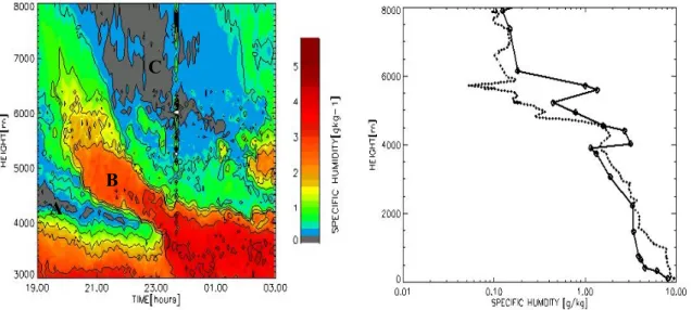
The time evolution of the water vapor mixing ratio, measured 30 h later by the ISAC RMR LIDAR, is reported in Fig. 1 and plotted as a succession of 15-min averaged

(10)

ACPD

4, 8327–8355, 2004

profiles; vertical smoothing is applied above 6000 m, with the effect of reducing the vertical resolution from 75 m to 525 m.

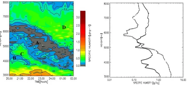
The water vapor exhibits a high variability during the measurement period and sev-eral layers are clearly noticeable. In particular, two distinct dry laminae are measured between 08:00 p.m. on 7 November and 02:00 a.m. the following day. The larger layer 5

(∼500 m thick, indicated by A in Fig. 1) in the middle-troposphere descends during the measurement from 6km to 4km in altitude with an apparent average fall speed of ∼250 m/h. The corresponding mixing ratio is less than 0.05 g/kg, a value definitely close to the limit of sensitivity of the ground based Raman system. This concentration indicates clear dehydration, up to one order of magnitude, compared to the average 10

concentration measured at these heights. Conversely, the upper layer between 6000– 8500 m (D), is variable throughout the measurement and exhibits typical tropospheric values of mixing ratio (∼0.5 g/kg). The second thin and dry tongue, with a water vapor concentration close to 0.1 g/kg, moves downward between 4 and 3.5 km (B), narrow-ing with time and disappearnarrow-ing after 11:00 p.m. Finally, a moist structure, embedded 15

between the A and B dry layers, is measured at 4 km (C) during the first 2 h of the observation.

Figure 1 also reports the humidity profiles from the high-resolution radiosoundings in Milano-LINATE, at 06:00 p.m. on 7 November and 00:00 a.m. the following day. A dry layer with a mixing ratio of ∼0.04 g/kg (and relative humidity reaching ∼2%) is observed 20

at ∼490 hPa (5800 m) at 06:00 p.m. The following soundings show that the layer moves downward with a behavior similar to that observed by LIDAR. The 00:00 a.m. profile shows, in agreement with LIDAR measurements, the presence of the moist substruc-tures at 5 km, embedded between the two dry layers. Nevertheless the water vapor structures measured by LIDAR and radiosounding appear to be temporally shifted, 25

consistent with the eastward displacement of the PV streamer.

LIDAR data measured the following night (between 8 and 9 November, not reported) show a residual dehydration of the troposphere above 6 km, while the evidence of laminar structures has vanished.

(11)

ACPD

4, 8327–8355, 2004

EGU

CETs are calculated backward from the LIDAR site, between 07:00 p.m. on 7 Novem-ber and 02:00 a.m. the following day, in order to cover the whole time and vertical range of the observations.

Results show that different ensembles of trajectories, converging in the Alps area, can be identified based on their geographical origins, water vapor and PV evolution. A 5

good match is found in altitude between the heights of trajectories and the observed atmospheric layers, characterized by different water vapor concentration. Trajectory clusters ending at the average altitude and time of the observed layers are selected and identified with the notation given if Fig. 1. The average values of altitude, PV, water vapor and geographical position are reported in Table 1 for the 72 h prior to the 10

LIDAR measurement, holding the longitude at 8.5◦E and the latitude ranging between 45◦–47◦N. The main features of each cluster are reported below:

A: Trajectories ending at an average altitude of 6400 m at 08:00 p.m., where the main dry layer is measured by LIDAR. These descend from an height ranging between 10 km and 11 km above the Hudson bay (Northern Canada); 72 h before the observations, the 15

average PV is 3.6 pvu and the specific humidity is 0.02 g/kg.

B: Trajectories ending in a range centered at 3.6 km in altitude at 20:00 UT, also characterized by high PV values (2.5 PV units) and low specific humidity (0.03 g/kg); these parcels originated from Greenland, descend from an altitude of 8500 m, 84 h before the measurements.

20

C: Trajectories ending between 4–5 km, are composed of two different groups con-verging in the observations area. The first group ascends from the lowermost tropo-sphere (2–3 km a.s.l.) and the geographical origin is above 60◦N latitude. The second group travels constantly south of 60◦N, in a range of heights between 5 km and 6 km.

D: Finally parcels corresponding to the moister layer above 7 km ascend from ∼6 km 25

and their water vapor content decrease along the path due to condensation effects. Based on this lagrangian analysis, the two dry layers detected by LIDAR appear to be generated by downward motion from UT-LS (Upper Troposphere-Lower Strato-sphere) region. This is highlighted by the signature in water vapor and PV, according

(12)

ACPD

4, 8327–8355, 2004

to the PV values (1.5–2.0 pvu) indicated in literature (e.g. Appenzeller et al., 1996) as representative of the dynamical tropopause.

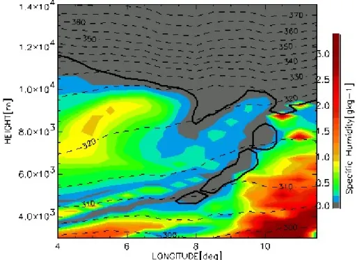
Figure 2 reports the water vapor vertical distribution obtained by LTR as a function of the longitude, at the latitude 46◦N, on 7 November at 15:00 UT, when the folding structure appears more evident. The whole structure moves eastward with time. Two 5

folds are clearly reproduced on PV and water vapor in agreement with the findings of Liniger and Davies (2003). Moreover, dry thin laminae, not evident in the reconstructed PV field, originate from the main streamer. The LTR is consistent with the LIDAR measurement (carried out at 8.5◦E) and in qualitative agreement with the observed water vapor layering: the LTR water vapor at the LIDAR coordinate clearly exhibits 10

two different dry layers originating from the upper tropospheric folding. Moreover, the LTR indicates a progressive descent of the main dry layer consistent in altitude and apparent vertical speed with the observed one.

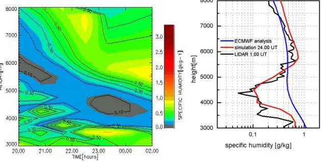
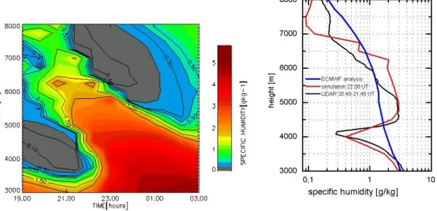
In order to compare the simulations and the observations on a quantitative basis, Fig. 3 reports the water vapor time evolution simulated by the LTR, simultaneously to 15

the LIDAR observations. The LTR water vapor shows the presence of the observed structures, in agreement with altitude, time, and water vapor concentration. The back-trajectory analysis confirms that LIDAR sampled the dry remnants of the PV streamer and that the moist “sandwiched” layer is composed of air originating from the lowermost maritime troposphere.

20

In the first part of simulation, below 5 km, a noisy distribution is obtained due the dispersion of trajectories ending at the corresponding altitude range.

Figure 3 also reports the direct comparison of the simultaneous vertical profile of water vapor (LIDAR, LTR and ECMWF) between 00:00 and 01:00 UT. The LTR profile is in good quantitative agreement with the measured one in the 4000–6000 m dry layer, 25

while the ECMWF profile does not show any evidence of dehydration in the 3000– 5000 m layer. The simulated water vapor is higher than the observed concentration in the driest part of the layer at 4800 m. In fact, the limited vertical resolution of the LTR (250 m) could inhibit the detailed reconstruction of the thinner observed layers.

(13)

ACPD

4, 8327–8355, 2004

EGU

5. 28 September 1999 case study

A PV anomaly above Europe, extending southward from the Scandinavian region, char-acterized the synoptic condition for about 24 h before LIDAR measurements were car-ried out in the night between 28 and 29 September 1999. The PV streamer centered on the Alpine region at 12:00 a.m. on 28 September and extending southward to 44◦N, 5

moved eastward with an horizontal velocity of about 30 km/h. At 06:00 p.m. the same day, the core of PV anomaly has completely passed over Northern Italy and was lo-cated above Eastern Europe (as seen in the isentropic PV map, not reported).

The LIDAR measurements are reported in Fig. 4. Consistent with the synoptic con-dition, at the beginning of the measurement (between 06.30 p.m. and 11:30 p.m.) a 10

dry layer (A) with values close to 0.09–0.1 g/kg is observed, moving downward from 5000 m to 4000 m. Its thickness decreases during the first four hours and it disappears afterwards. The Milano-Linate radiosounding, launched at 06:00 p.m., also exhibits the evidence of a dry layer at 500 hPa, with a mixing ratio of 0.07–0.09 g/kg (a relative humidity of 2–3%). The midnight radiosounding, only available at mandatory levels for 15

this day, shows an increase in the minimum relative humidity of 10% and values for the mixing ratio up to 0.4 g/kg.

In this case the disappearance of the dry layer can be explained by the synoptic evolution of the streamer, also leading to a transition from dry to moist conditions in the lowermost part of the troposphere.

20

The water vapor content inside this dry layer is definitely lower than the surrounding air; nevertheless, the observed concentration is greater than what would be expected in the lower stratosphere region.

An abrupt change in the condition is observed after 11:00 p.m. with a dramatic in-crease in water vapor concentration in the 3000–4000 m layer, from ∼0.1 g/kg to 4– 25

5 g/kg (B). Finally, a dry layer (C), descending from 8000 to 6000 m, is characterized by water vapor concentrations typical of upper-tropospheric conditions (0.2–0.3 g/kg).

(14)

ACPD

4, 8327–8355, 2004

used to identify the origin of the different layers. Three different CETs are identified. The average values of altitude, PV, specific humidity, potential temperature and latitude are reported in table 2 for the 48 h prior to the LIDAR measurement.

The main features are reported below:

A: Trajectories ending between 4250 m and 4750 m, at 08:00 p.m. experience a 5

downward transport from an altitude of 8000–10 000 m to arrive in the Alpine area they originated above an area between Iceland and Britain Islands. The mean PV values decrease along the trajectory from 3.5 PVU (PV Units) to 1 PVU. Conversely, the water vapor mixing ratio increases from 0.04 g/kg to 0.6 g/kg.

B: Trajectories ending in the same altitude as group A, but at 00:00 UT on 29 Septem-10

ber, exhibit the opposite characteristics. These originated in the Atlantic region, uplift from lower troposphere(∼2000 m) up to the middle troposphere (between 3000 and 7000 m height). The ending altitude of this cluster matches the position of the moist layer observed in the LIDAR data and progressively decreases with time in the following simulations.

15

C: Finally, the trajectories corresponding to the third dry layer, ending at 00:00 UT in the altitude range of 6.7 km–7.2 km, also originated from the upper troposphere but at a lower latitude. They appear to conserve upper tropospheric features (water vapor concentration and PV) and do not show evidences of a stratospheric origin.

The properties shown by the different groups of trajectories appear well related with 20

the distribution of water vapor measured by LIDAR at the corresponding heights and times.

In this case the PV appears more conserved along the trajectory, with respect to the case of 7 November; this is explained with the shorter life-time of the observed streamer.

25

Figure 5 reports the water vapor vertical distribution from LTR with the same char-acteristics as in Fig. 2. A dry and high PV streamer extends between 6◦E and 12◦E, descending at a height of 3500 m. The event is followed by moist air transport, with an indication of ascent in the moister layer at a height of 8000 m between 5◦E and 8◦E.

(15)

ACPD

4, 8327–8355, 2004

EGU

The LTR support the hypothesis that dehydration in the first part of LIDAR observa-tions is related to the intrusion event. In fact the dry layer (A) appears to be associated with the streamer at 4500 m and the substantial increase in water vapor is related to differential advection of moist air.

Figure 6 reports the water vapor time evolution simulated by the LTR as in Fig. 3. 5

The values of Potential Vorticity given by the simulation at the time of measurements, not shown, describe the exact correspondence between low water vapor concentration and maximum PV values (1.5–2.0 pvu) for the lowermost layer, that appears as the lower tip of the principal fold passing over the LIDAR site.

Vice versa the second dry layer on measurements and simulations in the range of 10

6–8 km shows values that are not representative of the stratosphere, suggesting that it is of a completely tropospheric origin.

6. Discussion and conclusions

The analysis of two LIDAR observations during the MAP 1999 campaign indicated the presence of dry layers penetrating deeply in the lowermost free troposphere. These 15

small scale structures (300 m–1 km) observed by Raman LIDAR are related to the pres-ence of upper tropospheric PV streamers and identified as filaments of air intruding from the lowermost stratosphere. The measurements were taken during the final stage of these events and the different layers detected by LIDAR cannot be observed in the conventional ECMWF meteorological analysis due to their coarse resolution. A 20

Lagrangian technique based on the principle of Reverse Domain Filling is used to sim-ulate the measured field resolving most of the observed layering.

The simulated field also allowed a direct comparison of the water vapor content and potential vorticity values inside the dry layers. The occurrence of a simultaneous low water vapor concentration and maximum Potential Vorticity inside the same layers, 25

along with the time-history of the corresponding back-trajectories confirms an origin from the lowermost stratosphere for these dry structures. For the 7 November case,

(16)

ACPD

4, 8327–8355, 2004

the occurrence of two distinct descending dry tongues is well identified and related to a double folding, also confirmed by the reconstructed Lagrangian PV field.

Following their temporal evolution, the dry filaments have been observed to narrow and penetrate deeply in the troposphere (the lowermost detected down to ∼3.5 km). Moreover the dry layers are interleaved by moister air. This feature appears consis-5

tent with that shown in the analysis of the same event at a previous stage (Liniger and Davies, 2003) simulated by analogous technique but not supported by the observa-tional evidence.

The values of mixing ratio measured inside the dry layers have been compared with those provided by ECMWF at the origin of the air parcels trajectory. The two layers 10

detected at the lower altitude (3–5 km), in both the two cases studied, appear char-acterized by values higher than those expected in the lower stratosphere, suggesting the occurrence of a progressive dilution of the air penetrating down through the tropo-sphere. Furthermore, simulations indicates that such layers are an extreme filamenta-tion of the fold, where strong mixing is expected (Browell et al., 1987). In addifilamenta-tion, the 15

behavior of chemical and dynamical parameters along the trajectory shows a loss of PV and an increase in water vapor along the 48–96 h paths.

This appears in agreement with that found in previous observational studies of ozone filaments persisting in the free troposphere (Vaughan et al., 2000; Bertin et al., 2001), that also indicates different behavior in the dissipation of chemical and dynamical trac-20

ers.

Lower values of mixing ratio are, instead, measured inside the upper dry layer on the 7 November case (∼0.05 g/kg). The comparison of these values with those at the origin of the trajectory, by ECMWF analysis, (∼0.03 g/kg), seems to indicate a less evident effect of dilution. Moreover, the LTR fields suggest a different behavior in the evolution 25

of UT-LS water vapor and Potential Vorticity along the trajectories: low concentration of water vapor appears to be better conserved than positive PV anomalies.

The orographic effect due to the interaction with the Alpine ridge could play a role in the streamer evolution. In fact, the Canadian MC2 limited area model (Benoit et al.,

(17)

ACPD

4, 8327–8355, 2004

EGU

1997) simulations (not reported and available athttp://www.map.ethz.ch) indicate that the PV layers originating from the tropopause folding are dissipated above the relief before the measurements.

Acknowledgements. P. D’Aulerio was supported by a PhD grant from the University of L’Aquila.

The author wishes to acknowledge ECMWF for providing the meteorological analyses and the 5

European Science Foundation for supporting the ACPD special issue. The authors wish to thank A. Buzzi for fruitful discussions.

References

Ancellet, G., Pelon, J., Beekmann, M., Papayannis, A., and Megie, G.: Ground-Based lidar studies of ozone exchanges between the stratosphere and the troposphere, J. Geophys. 10

Res., 96, 22 401–22 421, 1991.

Appenzeller, C. and Davies, H. C.: Structure of stratospheric intrusion into the troposphere, Nature, 358, 570–572, 1992.

Appenzeller, C., Davies, H. C., and Norton, W. A.: Fragmentation of stratospheric intrusions, J. Geophys. Res., 101, 1435–1456, 1996.

15

Benoit, R., Desgagn ´e, M., Pellerin, P., Pellerin, S., Desjardins, S., and Chartier, Y.: The Cana-dian MC2: a semi-Lagrangian, semi-implicit wide-band atmospheric model suited for fine-scale process studies and simulation. Mon. Weather. Rev., 125, 2382–2415, 1997.

Bertin, F., Campistron, B., Caccia, J. L, and Wilson, R.: Mixing processes in a tropopause folding observed by a network of ST radar and lidar, Ann. Geophys., 19, 953–963, 2001, 20

SRef-ID: 1432-0576/ag/2001-19-953.

Bithell, M., Vaughan, G., and Gray, L. J.: Persistence of stratospheric ozone layers in the troposphere, Atmos. Envir., 34, 2563–2570, 2000.

Bougeault, P., Binder, P., Buzzi, A., Dirks, R., Houze, R., Kuettner, J., Smith, R. B., Steinacker, R., and Volkert, H.: The MAP Special Observing Period, Bull. Amer. Meteor. Soc., 82, 433– 25

462, 2002.

Browell, E. V., Danielsen, E. F., Ismail, S., Gregory, G. L., and Bleck, S. M.: Tropopause fold structure determinated from airborn lidar and in situ measurements, J. Geophys. Res., 92, 2112–2120, 1987.

(18)

ACPD

4, 8327–8355, 2004

Buzzi, A., D’Isidoro, M., and Davolio, S.: A case study of an orographic cyclone south of the Alps during the MAP-SOP Q. J. R. Meteorol. Soc., 129, 1795–1818, 2003.

Congeduti, F., Medaglia, C. M., D’Aulerio, P., Fierli, F., Casadio, S., Baldetti, P., and Belardinelli, F.: A powerful trasportable Rayleigh-Mie-Raman LIDAR System, International Laser Radar Conference, edited by: Bissonette, L., Roy, G., Vall ´ee, G., Defence R&D, Quebec, Canada, 5

2002.

Cox, B. D., Bithell, M., and Gray, L. J.: A general circulation model study of a tropopause folding event at middle latitudes, Q.J.R. Meteorol. Soc., 121, 883–910, 1995.

Danielsen, E. F.: Stratospheric-Tropospheric Exchange bases based upon radioactivity, ozone and Potential Vorticity, J. Atmos. Sci., 25, 502–518, 1968.

10

Dragani, R., Redaelli, G., Visconti, G., Mariotti, A., Rudakov, V., MacKenzie, A. R., and Ste-fanutti, L.: High-Resolution Stratospheric Tracer Field Reconstructed with Lagrangian Tech-niques: A Comparative Analysis of Predictive Skill, J. Atmos. Sci., 59, 1943–1958, 2002. Eisele, H., Scheel, H. E., Sladkovic, R., and Trickl, T.: High Resolution lidar measurements of

stratosphere-troposphere exchange, J. Atmos. Sci., 56, 319–330, 1999. 15

Forster, C. and Wirth, V.: Radiative decay of an idealized stratospheric filaments in the tropopo-sphere, J. Geophys. Res., 105, 10 169–10 184, 2000.

Gray, L. J., Bithell, M., and Cox, B. D.: The role of specific humidity fields in the diagnosis of stratosphere troposphere exchange, Geophys. Res. Lett., 21, 2103–2106, 1994.

Hoinka, K. P., Richard, E., Poberaj, G., Busen, R., Caccia, J.-L., Fix, A., and Mannstein, H.: 20

Analysis of a potential vorticity streamer crossing the Alps during MAP IOP-15 on 6 Novem-ber 1999, Q. J. R. Meteorol. Soc., 129, 609–632, 2003.

Holton, J., Haynes, P. H., McIntyre, M. E., Douglass, A. R., Rood, R. B., and Pfister, L.: Stratosphere-Troposphere Exchange, Rev. Geophys., 33, 403–439, 1995.

Knudsen, B. M. and Carver, G. D.: Accuracy of the isentropic trajectories calculated for the 25

EASOE campaign, Geophys. Res. Lett., 21, 1199–1202, 1994.

Langfort, A. O. and Reid, S. J.: Dissipation and mixing of a small-scale stratospheric intrusion in the upper troposphere, J. Geophys. Res., 103, 31 265–31 276, 1998.

Liniger, M. and Davies, H. C.: Sub-Structure of a MAP streamer, Q. J. R. Meteorol. Soc., 129, 633–651, 2003.

30

Manney, G. L., Bird, J. C., Donovan, D. P., Duck, T. J., Whiteway, J. A., Pal, S. R., and Carswell, A. I.: Modeling ozone laminae in ground-based Artic wintertime observations using trajectory calculations and satellite data, J. Geophys. Res., 103, 5797–5814, 1998.

(19)

ACPD

4, 8327–8355, 2004

EGU

Massacand, A. C., Wernli, H., and Davies, H. C.: Heavy precipitation on the Alpine South side: An upper-level precursor, Geophys. Res. Lett., 25, 1435–1438, 1998.

Methven, J., Arnold, S. R., O’Connor, F. M., Barjat, H., Dewey, K., Kent, J., and Brough, N.: Estimating photochemically produced ozone throughout a domain using flight data and a Lagrangian model, J. Geophys. Res., 108 (D9), 4271, doi:10.1029/2002JD002955, 2003. 5

Newell, R. E., Thouret, V., Cho, J. Y. N., Stoller, P., Marenco, A., and Smit, H. G.: Ubiquity of quasi horizontal layers in the troposphere, Nature, 398, 316–319, 1999.

Orsolini, Y. J., Manney, G. L, Engel, A., Ovarlez, J., Claud, C., and Coy, L.: Layering in strato-spheric profiles of long-lived trace species: Ballon-borne observations and modeling, J. Geo-phys. Res., 103, 5815–5825, 1998.

10

Pierrehumbert, R. T.: Lateral Mixing ratio as a source of subtropical tropospheric water vapor, Geophys. Res. Lett., 25, 151–154, 1998.

Ravetta, F. and Ancellet, G.: Identification of dynamical processes at the tropopause during the decay of a cut-off low using high resolution airborne lidar measurements, Mon. Wea. Rev., 128, 3252–3267, 2000.

15

Shapiro, M. A.: Turbulent mixing within tropopause folds as mechanism for the exchange of chemical constituents between the stratosphere and troposphere, J. Atmos. Sci., 37, 994– 1004, 1980.

SPARC Assessment of Upper Tropospheric and Stratospheric Water Vapour, edited by: Kley, D., Russell III, J. M., and Phillips, C., WMO/TD-No. 1043, SPARC Report No. 2, 2000. 20

Stohl, A.: Computation, accuracy and application of trajectories-a review and bibliography, Atmos. Envir., 32, 947–966, 1998.

Stohl, A., Bonasoni, P., Cristofanelli, P., Collins, W., Feichter, J., Frank, A., Forster, C., Gera-sopoulos, E., Gaggeler, H., James, P., Kentarchos, T., Kreipl, S., Kromp-Kolb, H., Kruger, B., Land, C., Meloen, J., Papayannis, A., Priller, A., Seibert, P., Sprenger, M., Roelofs, G. J., 25

Scheel, E., Schnabel, C., Siegmund, P., Tobler, L., Trickl, T., Wernli, H., Wirth, V., Zanis, P., and Zerefos, C.: Stratosphere-troposphere exchange – a review, and what we have learned from STACCATO, J. Geophys. Res., 108, D12, 8516, 2003.

Sutton, R. T., Maclean, H., Swinbank, R., O’Neill, A., and Taylor, F. W.: High resolution strato-spheric tracer fields estimated from satellite observations using Lagrangian trajectory calcu-30

lations, J. Atmos. Sci., 51, 2995–3005, 1994.

Vaughan, G. and Worthington, R. M.: Break-up of a stratospheric streamer observed by MST radar, Q.J.R. Meteorol. Soc., 126, 1751–1769, 2000.

(20)

ACPD

4, 8327–8355, 2004

Vaughan, G., Price, J. D., and Howells, A.: Transport into the troposphere in a tropopause fold, Q.J.R. Meteorol. Soc., 120, 1085–1103, 1994.

Wernli, H. and Davies, H. C.: A lagrangian based analysis of extra tropical cyclones I: The method and some applications, Q.J.R. Meteorol. Soc., 123, 467–489, 1997.

Whiteman, D. N., Melfi, S. H., and Ferrare, R. A.: Raman lidar system for the measurement of 5

(21)

ACPD

4, 8327–8355, 2004

EGU

Table 1. Time history for the groups of trajectories ending at 8.5◦E (45–47◦N) in different ranges of altitude. The table includes mean values and standard deviations of height, PV, specific humidity, potential temperature and latitude, every 12 h.

Time [h] Alt [m] PV [p.v.u.] Q [g/kg] θ [K] LAT [deg] GROUP A: 6250 m–6750 m t=0→20:00 UT 0 6531±208 0.35±0.08 0.24±0.02 315.6±0.5 45.6 −12 7551±141 0.28±0.08 0.22±0.07 316.4±0.6 57.9 −24 7378±228 0.40±0.10 0.10±0.03 316.4±0.5 55.2 −36 7695±267 1.10±0.20 0.06±0.02 316.7±0.3 45.1 −48 7536±427 1.10±0.30 0.05±0.02 318.4±0.6 38.6 −60 9007±480 1.30±0.20 0.03±0.001 318.9±0.8 42.0 −72 10 116±128 3.60±0.60 0.0212±0.0005 321.0±1.0 51.8 GROUP B: 3500 m–3750 m t=0→20:00 UT 0 3625±136 0.90±0.20 1.16±0.05 301.5±1.7 46.0 −12 4368±312 0.81±0.05 0.75±0.19 302.2±1.9 50.7 −24 5407±335 0.90±0.20 0.28±0.11 302.8±1.7 58.4 −36 5162±393 1.10±0.20 0.29±0.12 304.1±1.3 55.1 −48 4803±132 1.30±0.10 0.19±0.04 305.1±1.0 47.3 −60 4926±65 1.60±0.09 0.069±0.008 307.1±1.2 55.4 −72 7302±420 1.70±0.30 0.040±0.006 309.2±0.5 67.0

(22)

ACPD

4, 8327–8355, 2004

Table 1. Continued.

Time [h] Alt [m] PV [p.v.u.] Q [g/kg] θ [K] LAT [deg] GROUP C1: 4250 m–5500 m t=0→20:00 UT 0 4875±410 0.74±0.11 0.46±0.16 309.0±2.2 45.4 −12 5682±368 1.07±0.15 0.24±0.07 309.8±2.3 54.0 −24 6073±356 0.45±0.38 0.22±0.08 312.2±2.1 61.5 −36 6901±890 0.27±0.16 0.32±0.17 312.7±2.4 65.5 −48 7203±1200 0.30±0.47 0.45±0.48 313.0±3.2 65.5 −60 4219±944 0.40±0.10 2.65±0.97 307.5±3.0 58.9 −72 2863±753 0.53±0.33 4.25±1.69 304.5±3.7 52.6 GROUP C2: 4250 m–5500 m t=0→20:00 UT 0 5071±313 0.72±0.18 0.28±0.04 310.0±1.5 46.2 −12 5984±256 0.78±0.09 0.25±0.05 311.1±1.4 56.5 −24 5618±268 0.61±0.05 0.24±0.04 312.7±1.2 59.2 −36 5008±226 0.58±0.04 0.21±0.04 312.9±1.2 54.0 −48 5210±320 0.58±0.03 0.21±0.03 313.5±1.2 46.6 −60 5522±258 0.58±0.08 0.15±0.07 314.1±1.3 40.0 −72 5834±372 0.78±0.22 0.15±0.14 315.3±1.6 36.9

(23)

ACPD

4, 8327–8355, 2004

EGU

Table 1. Continued.

Time [h] Alt [m] PV [p.v.u.] Q [g/kg] θ [K] LAT [deg] GROUP D: 7500 m–8000 m t=0→23:00 UT 0 7750±211 0.08±0.04 0.25±0.02 319.4±0.7 46.0 −12 8437±160 0.20±0.04 0.27±0.03 320.2±0.8 58.4 −24 7186±224 0.40±0.13 0.71±0.19 319.4±1.4 52.9 −36 6142±430 0.52±0.19 1.12±0.57 315.8±1.1 45.3 −48 5756±387 0.27±0.06 1.03±0.65 316.3±0.9 40.5 −60 5414±529 0.26±0.05 0.80±0.61 317.1±0.5 36.6 −72 5348±465 0.27±0.09 0.68±0.66 318.4±0.3 34.1

(24)

ACPD

4, 8327–8355, 2004

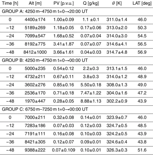
Table 2. As Table 1 for trajectories ending on 28 September at 20:00 and on 29 September at 00:00 UT.

Time [h] Alt [m] PV [p.v.u.] Q [g/kg] θ [K] LAT [deg] GROUP A: 4250 m–4750 m t=0→20:00 UT 0 4400±174 1.00±0.09 1.1 ±0.1 311.0±1.4 46.0 −12 5189±269 1.18±0.05 0.17±0.06 313.0±2.0 50.3 −24 7099±547 1.68±0.52 0.07±0.04 314.0±3.0 54.5 −36 8192±775 3.41±1.87 0.07±0.07 314.6±4.1 56.5 −48 8412±1000 3.66±1.61 0.04±0.03 314.7±4.8 56.9 GROUP B: 4250 m–4750 m t=0→00:00 UT 0 5000±235 0.54±0.12 2.2±0.3 313.1±1.5 46.0 −12 4732±211 0.67±0.11 3.8±0.3 314.0±1.2 48.9 −24 3602±276 0.85±0.16 5.50±0.18 308.0±1.3 49.0 −36 2536±170 0.71±0.18 7.47±1.22 304.0±1.6 47.2 −48 1970±447 0.28±0.05 8.88±1.13 302.2±0.9 43.9 GROUP C: 6750 m–7250 m t=0→00:00 UT 0 7000±211 0.32±0.08 0.14±0.01 323.9±0.7 46.0 −12 7283±186 0.07±0.03 0.12±0.03 324.7±0.5 48.5 −24 7191±111 0.16±0.08 0.10±0.03 324.2±0.5 43.9 −36 8421±305 0.12±0.07 0.09±0.01 324.6±0.4 43.8 −48 9388±222 0.07±0.109 0.10±0.01 326.3±0.3 51.6

(25)

ACPD

4, 8327–8355, 2004

EGU

21

Figure 1. Time evolution of water vapor vertical profiles measured by LIDAR from the 7th of November, 1999 at 20.00 UT until 8th of November at 2.00 UT. The color code corresponds to the specific humidity. On the right specific humidity profiles measured in Milano Linate at 18.00 (dotted line) and 00.00 (bold line) are shown.

A C

D

B

Fig. 1. Time evolution of water vapor vertical profiles measured by LIDAR from 7 November 1999 at 20:00 UT until 8 November at 02:00 UT. The color code corresponds to the specific humidity. On the right specific humidity profiles measured in Milano Linate at 18:00 (dotted line) and 00:00 UT (bold line) are shown.

(26)

ACPD

4, 8327–8355, 2004

Fig. 2. W-E oriented cross section along 46◦N showing the residual tropopause fold on 7 November at 15:00 UT. Color code corresponds to specific humidity, the black continuous line corresponds to 1.5 PVU (as obtained by LTR) and the dotted lines indicate potential tempera-ture levels (every 5 K). The LIDAR site is based at 8.5◦E at the center of x-axis.

(27)

ACPD

4, 8327–8355, 2004

EGU

23 Figure 3. Water vapor time evolution as simulated by the LTR in the interval 20.00-2.00 UT

for November 7

th

(left). On the right comparison of water vapor vertical profiles from 1hour

integrated LIDAR (black line), LTR simulation (red line) and ECMWF analysis (blue line) is

shown.

Fig. 3. Water vapor time evolution as simulated by the LTR in the interval 20:00–02:00 UT for 7 November (left). On the right comparison of water vapor vertical profiles from 1hour integrated LIDAR (black line), LTR simulation (red line) and ECMWF analysis (blue line) is shown.

(28)

ACPD

4, 8327–8355, 2004

EGU

Figure 4. Time evolution of water vapor vertical profiles measured by LIDAR from the 28 of October, 1999 at 19.00 UT until 29 of September at 3.00 UT. The color code corresponds to the specific humidity . On the right specific humidity profiles measured in Milano Linate at 18.00 (dotted line) and 00.00 (bold line) are shown.

A

B C

Fig. 4. Time evolution of water vapor vertical profiles measured by LIDAR from 28 October 1999 at 19:00 UT until 29 September at 03:00 UT. The color code corresponds to the specific humidity. On the right specific humidity profiles measured in Milano Linate at 18:00 (dotted line) and 00:00 UT (bold line) are shown.

(29)

ACPD

4, 8327–8355, 2004

EGU

(30)

ACPD

4, 8327–8355, 2004

EGU

Figure 6. Water vapor time evolution as simulated by the LTR in the interval 19.00 UT-3.00 UT for September 28 (left). On the right comparison of water vapor vertical profiles from 1hour integrated LIDAR (black line), LTR simulation (red line) and ECMWF analysis (blue line) is shown.

Fig. 6. Water vapor time evolution as simulated by the LTR in the interval 19:00 UT–03:00 UT for 28 September (left). On the right comparison of water vapor vertical profiles from 1hour integrated LIDAR (black line), LTR simulation (red line) and ECMWF analysis (blue line) is shown.