HAL Id: inria-00132988
https://hal.inria.fr/inria-00132988v8
Submitted on 18 Feb 2008
HAL is a multi-disciplinary open access
archive for the deposit and dissemination of
sci-L’archive ouverte pluridisciplinaire HAL, est
destinée au dépôt et à la diffusion de documents
guards
Menelaos Karavelas, Elias Tsigaridas
To cite this version:
Menelaos Karavelas, Elias Tsigaridas. Guarding curvilinear art galleries with vertex or point guards.
[Research Report] RR-6132, INRIA. 2007. �inria-00132988v8�
a p p o r t
d e r e c h e r c h e
Thème SYM
Guarding curvilinear art galleries with vertex or
point guards
Menelaos I. Karavelas — Elias P. Tsigaridas
N° 6132
Menelaos I. Karavelas
∗ †, Elias P. Tsigaridas
‡ §Thème SYM — Systèmes symboliques Projet VEGAS
Rapport de recherche n° 6132 — February 2007 — 39 pages
Abstract: One of the earliest and most well known problems in computational geometry is the so-called art gallery problem. The goal is to compute the minimum possible number guards placed on the vertices of a simple polygon in such a way that they cover the interior of the polygon. We consider the problem of guarding an art gallery which is modeled as a polygon with curvilinear walls. Our main focus is on polygons the edges of which are convex arcs pointing towards the exterior or interior of the polygon (but not both), named piecewise-convex and piecewise-concave polygons. We prove that, in the case of piecewise-convex polygons, if we only allow vertex guards,⌊4n
7⌋ − 1
guards are sometimes necessary, and⌊2n
3⌋ guards are always sufficient. Moreover, an O(n log n)
time and O(n) space algorithm is described that produces a vertex guarding set of size at most ⌊2n 3 ⌋.
When we allow point guards the afore-mentioned lower bound drops down to⌊n
2⌋. In the special
case of monotone piecewise-convex polygons we can show that⌊n
2⌋ + 1 vertex or ⌊ n
2⌋ point guards
are always sufficient and sometimes necessary. In the case of piecewise-concave polygons, we show that2n − 4 point guards are always sufficient and sometimes necessary, whereas it might not be
possible to guard such polygons by vertex guards. We conclude with bounds for other types of curvilinear polygons and future work.
Key-words: art gallery, curvilinear polygons, vertex guards, point guards, piecewise-convex
poly-gons, piecewise-concave polygons
This work is partially supported by the european project ACS (Algorithms for Complex Shapes, IST FET Open 006413) and ARC ARCADIA (http://www.loria.fr/∼petitjea/Arcadia/)
∗University of Crete, Department of Applied Mathematics, GR-714 09 Heraklion, Greece
†Foundation for Research and Technology - Hellas, Institute of Applied and Computational Mathematics P.O. Box 1385,
GR-711 10 Heraklion, Greece
‡LORIA-INRIA Lorraine, Nancy, FRANCE
ou de point
Résumé : Un des plus anciens et plus célèbres problèmes en géométrie algorithmique est le
prob-lème dit de galerie d’art qui consiste à calculer le nombre minimal des gardians qui sont nécessaires afin de couvrir l’intérieur d’un polygone simple s’ils sont placés sur ses sommets.
Dans cet article, nous considérons le problème de garde d’une galerie d’art qui est modélisée par un polygone avec des murs courbés. En particulier, nous considérons des polygones dont les bords sont des arcs convexes qui se dirigent vers l’extérieur ou l’intérieur du polygone (mais pas les deux au même temps), appelés polygones par morceaux convexes ou concaves respectivement. Nous montrons que, dans le cas de polygones par morceaux convexes, si nous permettons seulement des gardians de sommets, alors⌊4n
7⌋−1 gardians sont parfois nécessaires, et ⌊ 2n
3 ⌋ gardians sont toujours
suffisants. D’ailleurs, nous décrivons un algorithme, O(n log n) en temps et O(n) en espace, qui
produit l’ensemble des sommets de garde de taille au plus⌊2n
3⌋. Dans le cas particulier de polygones
monotones et par morceaux convexes nous pouvons montrer que⌊n
2⌋ + 1 gardians de sommets ou
⌊n
2⌋ gardians de points sont toujours suffisants et parfois nécessaires.
Dans le cas des polygones par morceaux concaves, nous prouvons que2n − 4 gardians de points
sont toujours suffisantes et parfois nécessaires, tandis qu’il ne peut être possible de garder de tels polygones par des gardians de sommets. Nous concluons avec des limites pour d’autres types de polygones courbés et perspectives pour le futur.
Mots-clés : galerie d’art; polygones courbés, gardians de sommet, gardians de point, polygones par
1
Introduction
Consider a simple polygon P with n vertices. How many points with omnidirectional visibility are required in order to see every point in the interior of P ? This problem, known as the art gallery problem has been one of the earliest problems in Computational Geometry. Applications areas include robotics [21, 36], motion planning [24, 28], computer vision and pattern recognition [32, 37, 2, 33], graphics [26, 7], CAD/CAM [4, 15] and wireless networks [16]. In the late 1980’s to mid 1990’s interest moved from linear polygonal objects to curvilinear objects [35, 9, 11, 10] — see also the paper by Dobkin and Souvaine [13] that extends linear polygon algorithms to curvilinear polygons, as well as the recent book by Boissonnat and Teillaud [3] for a collection of results on non-linear computational geometry beyond art gallery related problems. In this context this paper addresses the classical art gallery problem for various classes of polygonal regions the edges of which are arcs of curves. To the best of our knowledge this is the first time that the art gallery problem is considered in this context.
The first results on the art gallery problem or its variations date back to the 1970’s. Chvátal [8] was the first to prove that a simple polygon with n vertices can be always guarded with⌊n
3⌋ vertices;
this bound is tight in the worst case. The proof by Chvátal was quite tedious and Fisk [18] gave a much simpler proof by means of triangulating the polygon and coloring its vertices using three colors in such a way so that every triangle in the triangulation of the polygon does not contain two vertices of the same color. The algorithm proposed by Fisk runs in O(T (n) + n) time, where T (n) is the
time to triangulate a simple polygon. Following Chazelle’s linear-time algorithm for triangulating a simple polygon [5, 6], the algorithm proposed by Fisk runs in O(n) time. Lee and Lin [22] showed
that computing the minimum number of vertex guards for a simple polygon is NP-hard, which was extended to point guards by Aggarwal [1]. Soon afterwards other types of polygons were considered. Kahn, Klawe and Kleitman [19] showed that orthogonal polygons of size n, i.e., polygons with axes-aligned edges, can be guarded with⌊n
4⌋ vertex guards, which is also a lower bound. Several O(n)
algorithms have been proposed for this variation of the problem, notably by Sack [30], who gave the first such algorithm, and later on by Lubiw [25]. Edelsbrunner, O’Rourke and Welzl [14] gave a linear time algorithm for guarding orthogonal polygons with⌊n
4⌋ point guards.
Beside simple polygons and simple orthogonal polygons, polygons with holes, and orthogonal polygons with holes have been investigated. As far as the type of guards is concerned, edge guards and mobile guards have been considered. An edge guard is an edge of the polygon, and a point is visible from it if it is visible from at least one point on the edge; mobile guards are essentially either edges of the polygon, or diagonals of the polygon. Other types of guarding problems have also been studied in the literature, notably, the fortress problem (guard the exterior of the polygon against enemy raids) and the prison yard problem (guard both the interior and the exterior of the polygon which represents a prison: prisoners must be guarded in the interior of the prison and should not be allowed to escape out of the prison). For a detailed discussion of these variations and the corresponding results the interested reader should refer to the book by O’Rourke [29], the survey paper by Shermer [31] and the book chapter by Urrutia [34].
In this paper we consider the original problem, that is the problem of guarding a simple polygon. We are primarily interested in the case of vertex guards, although results about point guards are also
described. In our case, polygons are not required to have linear edges. On the contrary we consider polygons that have smooth curvilinear edges. Clearly, these problems are NP-hard, since they are direct generalizations of the corresponding original art gallery problems. In the most general setting where we impose no restriction on the type of edges of the polygon, it is very easy to see that there exist curvilinear polygons that cannot be guarded with vertex guards, or require an infinite number of point guards (see Fig. 23(b)). Restricting the edges of the polygon to be locally convex curves, pointing towards the exterior of the polygon (i.e., the polygon is a locally convex set, except possibly at the vertices) we can construct polygons that require a minimum of n vertex or point guards, where
n is the number of vertices of the polygon (see Fig. 23(a)); in fact such polygons can always be
guarded with their n vertices. The main focus of this paper is the class of polygons that are either locally convex or locally concave (except possibly at the vertices), the edges of which are convex arcs; we call such polygons piecewise-convex and piecewise-concave polygons, respectively.
For the first class of polygons we show that it is always possible to guard them with⌊2n 3 ⌋
ver-tex guards, where n is the number of polygon vertices. On the other hand we describe families of piecewise-convex polygons that require a minimum of⌊4n
7⌋ − 1 vertex guards and ⌊ n
2⌋ point guards.
Aside from the combinatorial complexity type of results, we describe an O(n log n) time and O(n)
space algorithm which, given a piecewise-convex polygon, computes a guarding set of size at most
⌊2n
3⌋. Our algorithm should be viewed as a generalization of Fisk’s algorithm [18]; in fact, when
ap-plied to polygons with linear edges, it produces a guarding set of size at most⌊n
3⌋. For the purposes
of our complexity analysis and results, we assume, throughout the paper, that the curvilinear edges of our polygons are arcs of algebraic curves of constant degree; as a result all predicates required by the algorithms described in this paper take O(1) time in the Real RAM computation model. The central
idea for both obtaining the upper bound as well as for designing our algorithm is to approximate the piecewise-convex polygon by a linear polygon (a polygon with line segments as edges). Additional auxiliary vertices are added on the boundary of the curvilinear polygon in order to achieve this. The resulting linear polygon has the same topology as the original polygon and captures the essentials of the geometry of the piecewise-convex polygon; for obvious reasons we term this linear polygon the polygonal approximation. Once the polygonal approximation has been constructed, we compute a guarding set for it by applying a slight modification of Fisk’s algorithm [18]. The guarding set just computed for the polygonal approximation turns out to be a guarding set for the original curvilinear polygon. The final step of both the proof and our algorithm consists in mapping the guarding set of the polygonal approximation to another vertex guarding set consisting of vertices of the original polygon only.
If we further restrict ourselves to monotone piecewise-convex polygons, i.e., piecewise-convex polygons that have the property that there exists a line L, such that any line L⊥perpendicular to L intersects the polygon at most twice, we can show that⌊n
2⌋+1 vertex or ⌊n2⌋ point guards are always
sufficient and sometimes necessary. Such a line L can be computed in O(n) time (cf. [13]). Given L, it is very easy to compute a vertex guarding set of size⌊n
2⌋+1, or a point guarding set of size ⌊n2⌋:
the problem of computing such a guarding set essentially reduces to merging two sorted arrays, thus taking O(n) time and O(n) space. This result should be contrasted against the case of monotone
linear polygons where the corresponding upper and lower bound on the number of vertex or point guards required to guard the polygon matches that of general (i.e., not necessarily monotone) linear
polygons. In other words, monotonicity seems to play a crucial role in the case of piecewise-convex polygons, which is not the case for linear polygons.
For the second class of polygons, i.e., the class of piecewise-concave polygons, vertex guards may not be sufficient in order to guard the interior of the polygon (see Fig. 22(a)). We thus turn our attention to point guards, and we show that2n − 4 point guards are always sufficient and
some-times necessary. Our method for showing the sufficiency result is similar to the technique used to illuminate sets of disjoint convex objects on the plane [17]. Given a piecewise-concave polygon P , we construct a new locally concave polygon Q, contained inside P , and such that the tangencies between edges of Q are maximized. The problem of guarding P then reduces to the problem of guarding Q, which essentially consists of a number of faces with pairwise disjoint interiors. The faces of Q require, each, two point guards in order to be guarded, and are in 1–1 correspondence with the triangles of an appropriately defined triangulation graphT (R) of a polygon R with n
ver-tices. Thus the number point guards required to guard P is at most two times the number of faces of
T (R), i.e., 2n − 4.
The rest of the paper is structured as follows. In Section 2 we introduce some notation and provide various definitions. In Section 3 we present our algorithm for computing a guarding set, of size⌊2n
3 ⌋, for a piecewise-convex polygon with n vertices. Section 3 is further subdivided into five
subsections. In Subsection 3.1 we define the polygonal approximation of our curvilinear polygon and prove some geometric and combinatorial properties. In Subsection 3.2 we show how to construct a, properly chosen, constrained triangulation of the polygonal approximation. In Subsection 3.3 we describe how to compute the guarding set for the original curvilinear polygon from the guarding set of the polygonal approximation due to Fisk’s algorithm and prove the upper bound on the cardinality of the guarding set. In Subsection 3.4 we show how to compute the guarding set in O(n log n) time
and O(n) space. Finally, in Subsection 3.5 is devoted to the presentation of the family of polygons
that attains the lower bound of ⌊4n
7⌋ − 1 vertex guards. The special case of guarding monotone
piecewise-convex polygons is discussed in Section 4. We show that⌊n
2⌋ + 1 vertex (or ⌊ n 2⌋ point)
guards are always necessary and sometimes sufficient, and present an O(n) time and O(n) space
algorithm for computing such a guarding set. In Section 5 we present our results for piecewise-concave polygons, namely, that2n − 4 point guards are always necessary and sometimes sufficient
for this class of polygons. Section 6 contains further results. More precisely, we present bounds for locally convex polygons, monotone locally convex polygons and general polygons. The final section of the paper, Section 7, summarizes our results and discusses open problems.
2
Definitions
Curvilinear arcs. Let S be a sequence of points v1, . . . , vn and E a set of curvilinear arcs
a1, . . . , an, such that ai has as endpoints the points vi and vi+11. We will assume that the arcs
aiand aj, i6= j, do not intersect, except when j = i − 1 or j = i + 1, in which case they intersect
only at the points vi and vi+1, respectively . We define a curvilinear polygon P to be the closed
region delimited by the arcs ai. The points viare called the vertices of P . An arc aiis a convex arc
(a) (b) (c)
(d) (e) (f)
Figure 1: Different types of curvilinear polygons: (a) a linear polygon, (b) a convex polygon, (c) a piecewise-convex polygon, (d) a locally convex polygon, (e) a piecewise-concave polygon and (f) a general polygon.
if every line on the plane intersects aiat either at most two points or along a linear segment. If q is a
point in the interior of ai, an ε-neighborhood nε(q) of q is defined to be the intersection of aiwith a
disk centered at q with radius ε. An arc aiis a locally convex arc if for every point q in the interior of
ai, there exists an εqsuch that for every0 < ε ≤ εq, the ε-neighborhood of q lies entirely in one of
the two halfspaces defined by the line ℓ tangent to aiat q; note that if ℓ is not uniquely defined, then
the containment-in-halfspace property mentioned just above has to hold for any such line ℓ. Finally, note that a convex arc is also a locally convex arc.
Our definition does not really require that the arcs ai are smooth. In fact the arcs ai can be
polylines, in which case the results presented in this paper are still valid. What might be different, however, is our complexity analyses, since we have assumed that the ai’s have constant complexity.
In the remainder of this paper, and unless otherwise stated, we will assume that the arcs ai are
G1-continuous and have constant complexity.
Curvilinear polygons. A polygon P is a linear polygon if its edges are line segments (see Fig. 1(a)). A polygon P consisting of curvilinear arcs as edges is called a convex polygon if every line on the plane intersects its boundary at either at most two points or along a line segment (see Fig. 1(b)). A polygon is called a piecewise-convex polygon, if every arc is a convex arc and for every point q in the interior of an arc aiof the polygon, the interior of the polygon is locally on the same side as the
arc aiwith respect to the line tangent to aiat q (see Fig. 1(c)). A polygon is called a locally convex
polygon if the boundary of the polygon is a locally convex curve, except possibly at its vertices (see Fig. 1(d)). Note that a convex polygon is a piecewise-convex polygon and that a piecewise-convex
polygon is also a locally convex polygon. A polygon P is called a piecewise-concave polygon, if every arc of P is convex and for every point q in the interior of a non-linear arc ai, the interior of P
lies locally on both sides of the line tangent to aiat q (see Fig. 1(e)). Finally, a polygon is said to
be a general polygon if we impose no restrictions on the type of its edges (see Fig. 1(f)). We will use the term curvilinear polygon to refer to a polygon the edges of which are either line or curve segments.
Guards and guarding sets. In our setting, a guard or point guard is a point in the interior or on the boundary of a curvilinear polygon P . A guard of P that is also a vertex of P is called a vertex guard. We say that a curvilinear polygon P is guarded by a set G of guards if every point in P is visible from at least one point in G. The set G that has this property is called a guarding set for P . A guarding set that consists solely of vertices of P is called a vertex guarding set.
3
Piecewise-convex polygons
In this section we present an algorithm which, given a piecewise-convex polygon P of size n, it computes a vertex guarding set G of size⌊2n3⌋. The basic steps of the algorithm are as follows:
1. Compute the polygonal approximation ˜P of P .
2. Compute a constrained triangulationT ( ˜P) of ˜P .
3. Compute a guarding set GP˜for ˜P , by coloring the vertices ofT ( ˜P) using three colors.
4. Compute a guarding set GP for P from the guarding set GP˜.
3.1
Polygonalization of a piecewise-convex polygon
Let aibe a convex arc with endpoints vi and vi+1. We call the convex region ri delimited by ai
and the line segment vivi+1a room. A room is called degenerate if the arc aiis a line segment. A
line segment pq, where p, q ∈ ai is called a chord, and the region delimited by the chord pq and
ai is called a sector. The chord of a room ri is defined to be the line segment vivi+1 connecting
the endpoints of the corresponding arc ai. A degenerate sector is a sector with empty interior. We
distinguish between two types of rooms (see Fig. 2):
1. empty rooms: these are non-degenerate rooms that do not contain any vertex of P in the interior of rior in the interior of the chord vivi+1.
2. non-empty rooms: these are non-degenerate rooms that contain at least one vertex of P in the interior of rior in the interior of the chord vivi+1.
In order to polygonalize P we are going to add new vertices in the interior of non-linear convex arcs. To distinguish between the two types of vertices, the n vertices of P will be called original vertices, whereas the additional vertices will be called auxiliary vertices.
More specifically, for each empty room riwe add a vertex wi,1(anywhere) in the interior of the
r′ ne r′ e r′′ ne r′′ e
Figure 2: The two types of rooms in a piecewise-convex polygon: r′e and r′′e are empty rooms, whereas rne′ and r′′neare non-empty rooms.
v1 v2 v3 v4 v5 v6 v7 m5 a3 a5 r3 r5 w3,1 w5,1 w5,2
Figure 3: The auxiliary vertices (white points) for rooms r3 (empty) and r5 (non-empty). w3,1
is a point in the interior of a3. m5 is the midpoint of v5 and v6, whereas w5,1 and w5,2 are the
intersections of the lines m5v2 and m5v1 with the arc a5, respectively. In this example R5 =
{v1, v2, v7}, whereas C5∗= {v1, v2}.
interior of the chord vivi+1of ri, and Ribe the set of vertices of P that are contained in the interior
of rior belong to Xi(by assumption Ri6= ∅). If Ri6= Xi, let Cibe the set of vertices on the convex
hull of the vertex set(Ri\ Xi) ∪ {vi, vi+1}; if Ri = Xi, let Ci = Xi∪ {vi, vi+1}. Finally, let
C∗
i = Ci\ {vi, vi+1}. Clearly, viand vi+1belong to the set Ciand, furthermore, Ci∗6= ∅.
Let mi be the midpoint of vivi+1and ℓ⊥i (p) the line perpendicular to vivi+1passing through a
point p. If Ci∗6= Xi, then, for each vk ∈ Ci∗, let wi,jk,1 ≤ jk ≤ |C ∗
v1 v2 v3 v4 v5 v6 v7 w1,1 w2,1 w3,1 w5,1 w5,2 (a) v1 v2 v3 v4 v5 v6 v7 w1,1 w2,1 w3,1 w5,1 w5,2 (b)
Figure 4: (a) The polygonal approximation ˜P , shown in gray, of the piecewise-convex polygon P
with vertices vi, i= 1, . . . , 7. (b) The constrained triangulation T ( ˜P) of ˜P . The dark gray triangles
are the constrained triangles. The polygonal region v5w5,1w5,2v6v1v2v5is a crescent. The triangles
w5,1v2v5and v1w5,2v6are boundary crescent triangles. The triangle v2w5,2v1is an upper crescent
triangle, whereas the triangle v2w5,1w5,2is a lower crescent triangle.
of the line mivkwith the arc ai; if Ci∗ = Xi, then, for each vk ∈ Ci∗, let wi,jk,1 ≤ jk ≤ |C ∗ i|, be
the (unique) intersection of the line ℓ⊥i (vk) with the arc ai.
Now consider the sequence ˜S of the original vertices of P augmented by the auxiliary vertices
added to empty and non-empty rooms; the order of the vertices in ˜S is the order in which we
en-counter them as we traverse the boundary of P in the en-counterclockwise order. The linear polygon defined by the sequence ˜S of vertices is denoted by ˜P (see Fig. 4(a)). It is easy to show that: Lemma 1 The linear polygon ˜P is a simple polygon.
Proof. It suffices show that the line segments replacing the curvilinear segments of P do not intersect other edges of P or ˜P .
Let ri be an empty room, and let wi,1 be the point added in the interior of ai. The interior
of the line segments viwi,1 and wi,1vi+1 lie in the interior of ri. Since P is a piecewise-convex
polygon, and ri is an empty room, no edge of P could potentially intersect viwi,1 or wi,1vi+1.
Hence replacing aiby the polyline viwi,1vi+1gives us a new piecewise-convex polygon.
Let ri be a non-empty room. Let wi,1, . . . , wi,Ki be the points added on ai, where Ki is the
cardinality of Ci∗. By construction, every point wi,k is visible from wi,k+1, k= 1, . . . Ki− 1, and
every point wi,kis visible from wi,k−1, k= 2, . . . Ki. Moreover, wi,1is visible from viand wi,Ki
lie in the interior of ri and do not intersect any arc in P . Hence, substituting ai by the polyline
viwi,1. . . wi,Kivi+1gives us a new piecewise-convex polygon.
As a result, the linear polygon ˜P is a simple polygon. 2
We call the linear polygon ˜P , defined by ˜S, the straight-line polygonal approximation of P , or
simply the polygonal approximation of P . An obvious result for ˜P is the following:
Corollary 2 If P is a piecewise-convex polygon the polygonal approximation ˜P of P is a linear
polygon that is contained inside P .
We end this section by proving a tight upper bound on the size of the polygonal approximation of a piecewise-convex polygon. We start by stating and proving an intermediate result, namely that the sets Ci∗are pairwise disjoint.
Lemma 3 Let i, j, with1 ≤ i < j ≤ n. Then C∗
i ∩ Cj∗= ∅.
Proof. If one of the rooms riand rjis a degenerate or an empty room, the result is obvious.
Consider two non-empty rooms ri and rj. For simplicity of presentation we assume that Ri 6=
Xiand Rj6= Xj; the proof easily carries on to the case Ri = Xior Rj= Xj.
Suppose that there exists a vertex u ∈ P that is contained in C∗
i ∩ Cj∗. Let vi, vi+1, and
vj, vj+1 be the endpoints of the arcs ai and aj, and mi, mj the midpoints of the chords vivi+1,
vjvj+1, respectively. Let uibe the intersection of the line miu with the convex arc aiand ujbe the
intersection of the line mju with the convex arc aj, respectively. Consider the following cases.
vj, vj+1 6∈ Ri, vi, vi+1 6∈ Rj. This is the easy case (see Fig. 5). Since u∈ Ci∗∩ Cj∗ we have
that ri∩ rj 6= ∅. Moreover, it is either the case that aj intersects the chord vivi+1 or ai
intersects the chord vjvj+1. Without loss of generality we can assume that aj intersects the
chord vivi+1. In this case the boundary of ri∩ rjthat lies in the interior of riis a subarc of
aj. But then the segment uuihas to intersect aj, which contradicts the fact that u∈ Ci∗.
ai aj vi vi+1 vj vj+1 u ui mi
ai aj vi vi+1 vj vj+1 u ui mi (a) ai aj vi vi+1 vj vj+1 u ui mi (b) ai aj vi vi+1 vj v′ j vj+1 v′ j+1 u ui mi (c)
Figure 6: Proof of Lemma 3. The case vj, vj+1 ∈ Ri. (a) the chord vjvj+1intersects the interior
of uuiand u is contained inside the triangle vivi+1vj. (b) the chord vjvj+1intersects the interior of
uuiand u is contained inside the convex quadrilateral vivi+1vjvj+1. (c) the chord vjvj+1intersects
uuiat u.
vj, vj+1 ∈ Ri. Since u belongs to Ci∗, the line segment uuicannot contain any vertices of P and
it cannot intersect any edge of P (since otherwise u would not belong to Ci∗). For this reason, and since u belongs to Cj∗, uui has to intersect the chord of rj. We distinguish between the
following two cases (see Fig. 6):
1. The chord vjvj+1intersects the interior of uui. Depending on whether the supporting
line of vjvj+1intersects the chord vivi+1of rior not, u will be either contained in the
interior of one of the triangles vivi+1vj and vivi+1vj+1(this happens if the supporting
line of vjvj+1 intersects vivi+1 — see Fig. 6(a)), or inside the convex quadrilateral
vivi+1vjvj+1(this happens if the supporting line of vjvj+1does not intersect vivi+1—
see Fig. 6(b)). In either case, u is in the interior of a convex polygon, the vertices of which are in Ri∪ {vi, vi+1}, and, thus, it cannot belong to Ci∗, hence a contradiction.
2. The chord vjvj+1 intersects uui at u. We can assume without loss of generality that
vi+1, vjare to the right and vi, vj+1to the left of the oriented line uiu (see Fig. 6(c)).
Notice that both vjand vj+1have to belong to Ci∗, since otherwise u would not belong to
Ci∗. Let vj′ and vj+1′ be the intersections of the lines mivjand mivj+1with ai. Consider
the path π from u to vi on the boundary ∂P of P , that does not contain the edge aj.
π has to intersect either the interior of the line segment vjv′j or the interior of the line
segment vj+1vj+1′ ; either case yields a contradiction with the fact that both vjand vj+1
belong to Ci∗.
vi, vi+1 ∈ Rj. This case is symmetric to the previous one.
|{vj, vj+1} ∩ Ri| = 1. Without loss of generality we may assume that vj ∈ Riand vj+16∈ Ri.
ai aj vi vi+1 vj vj+1 u ui mi (a) ai aj vi vi+1 vj vj+1 v′ i v′ j u ui mi (b) ai aj vi vi+1 vj vj+1 v′ i+1 v′ j+1 u mi mj (c)
Figure 7: Proof of Lemma 3. The case|{vj, vj+1} ∩ Ri| = 1. (a) the chord vjvj+1intersects the
chord vivi+1and vjvj+1intersects the interior of vivi+1. (b) the chord vjvj+1intersects the chord
vivi+1and vjvj+1intersects vivi+1at vi. (c) the chord vjvj+1intersects ai.
1. The chord vjvj+1intersects the chord vivi+1. If vjvj+1intersects the interior of vivi+1
(see Fig. 7(a)), then u has to lie in the interior of the triangle vivi+1vj, which contradicts
the fact that u∈ C∗ i.
Suppose now that vjvj+1 intersects one of the endpoints of vivi+1, and let us assume
that this endpoint is vi(see Fig. 7(b)). u has to lie in the interior of vivj, since otherwise
it would have been in the interior of the triangle vivi+1vj, which contradicts the fact that
u∈ C∗
i. Moreover, vi(resp., vj) has to belong to Rj(resp., Ri), since otherwise u6∈ Cj∗
(resp., u 6∈ C∗
i). Let vj′ be the intersection of mivj with ai and v′ibe the intersection
with aj of the line perpendicular to vjvj+1at vi. Consider the paths π1and π2on ∂P
from u to vi+1and vj+1, respectively. One of these two paths has to intersect either the
interior of the line segment vivi′or the interior of line segment vjvj′; either case yields a
contradiction with the fact that vibelongs to Cj∗and vjbelongs to Ci∗.
2. The chord vjvj+1intersects the edge ai. In this case we also have that either vi ∈ Rj
or vi+1 ∈ Rj, but not both. Without loss of generality we may assume that vi+1 ∈ Rj
(see Fig. 7(c)). Since u belongs to both Ci∗ and Cj∗, it has to lie on the line segment
vi+1vj+1. Moreover, vj+1(resp., vi+1) has to belong to Ci∗(resp., Cj∗), since otherwise
u would not belong to C∗
i (resp., Cj∗). Let vi+1′ and vj+1′ be the intersections of the lines
mjvi+1and mivj+1with the arcs ajand ai, respectively. Consider the paths π1and π2
on ∂P from u to viand vj, respectively. One of these two paths has to intersect either
the interior of the line segment vi+1vi+1′ or the interior of the line segment vj+1v′j+1. In
the former case, we get a contradiction with the fact that vi+1belongs to Cj∗; in the latter
case we get a contradiction with the fact that vj+1belongs to Ci∗.
|{vi, vi+1} ∩ Rj| = 1. This case is symmetric to the previous one. 2
An immediate consequence of Lemma 3 is the following corollary that gives us a tight bound on the size of the polygonal approximation ˜P of P .
m1 v1 v2 v3 v4 v5 v6 vn−3 vn−2 vn−1 vn
Figure 8: A piecewise-convex polygon P of size n (solid curve), the polygonal approximation ˜P of
which consists of3n − 3 vertices (dashed polyline).
Corollary 4 If n is the size of a piecewise-convex polygon P , the size of its polygonal approximation ˜
P is at most3n. This bound is tight (up to a constant).
Proof. Let aibe a convex arc of P , and let ribe the corresponding room. If aiis an empty room, then
˜
P contains one auxiliary vertex due to ai. Hence ˜P contains at most n auxiliary vertices attributed to
empty rooms in P . If aiis a non-empty room, then ˜P contains|Ci∗| auxiliary vertices due to ai. By
Lemma 3 the sets Ci∗, i= 1, . . . , n are pairwise disjoint, which implies thatPn
i=1|Ci∗| ≤ |P | = n.
Therefore ˜P contains the n vertices of P , contains at most n vertices due to empty rooms in P and
at most n vertices due to non-empty rooms in P . We thus conclude that the size of ˜P is at most3n.
The upper bound of the paragraph above is tight up to a constant. Consider the piecewise-convex polygon P of Fig. 8. It consists of n− 1 empty rooms and one non-empty room r1, such that
|C∗
1| = n − 2. It is easy to see that | ˜P| = 3n − 3. 2
3.2
Triangulating the polygonal approximation
Let P be a piecewise-convex polygon and ˜P is its polygonal approximation. We are going to
con-struct a constrained triangulation of ˜P , i.e., we are going to triangulate ˜P , while enforcing some
triangles to be part of this triangulation. Let Pα = ˜P\ P be the set of auxiliary vertices in ˜P . The
main idea behind the way this particular triangulation is constructed is to enforce that:
1. all triangles ofT ( ˜P), that contain a vertex in Pα, also contain at least one vertex of P , i.e.,
no triangles contain only auxiliary vertices,
2. every vertex in Pαbelongs to at least one triangle inT ( ˜P) the other two vertices of which are
both vertices of P , and
3. the triangles ofT ( ˜P) that contain vertices of ˜P can be guarded by vertices of P .
These properties are going to be exploited in Step 4 of the algorithm presented in Section 3. More precisely, we are going to enforce the way the triangles ofT ( ˜P) are created in the
triangulate parts of ˜P . The remaining untriangulated parts of ˜P consist of one of more disjoint
poly-gons, which can then be triangulated by means of any O(n log n) polygon triangulation algorithm.
In other words, the triangulation of ˜P that we want to construct is a constrained triangulation, in the
sense that we pre-specify some of the edges of the triangulation. In fact, as we will see below we pre-specify triangles, rather than edges, which are going to be referred to as constrained triangles.
Let us proceed to define the constrained triangles inT ( ˜P). If ri is an empty room, and wi,1is
the point added on ai, add the edges vivi+1, viwi,1and wi,1vi+1, thus formulating the constrained
triangle viwi,1vi+1 (see Fig. 4(b)). If ri is a non-empty room,{c1, . . . , cKi} the vertices in C ∗ i,
Ki= |Ci∗|, and {wi,1, . . . , wi,Ki} the vertices added on ai, add the following edges, if they do not
already exist:
1. ck, ck+1, k= 1, . . . , Ki− 1; vic1; cKivi+1;
2. ciwi,k, k= 1, . . . , Ki;
3. ciwi,k+1, k= 1, . . . , Ki− 1;
4. wi,k, wi,k+1, k= 1, . . . , Ki− 1; viwi,1; wi,Kivi+1.
These edges formulate 2Ki constrained triangles, namely, ckck+1wi,k+1, k = 1, . . . , Ki − 1,
ckwi,kwi,k+1, k = 1, . . . , Ki − 1, vic1wi,1and vi+1cKiwi,Ki. We call the polygonal region
de-limited by these triangles a crescent. The triangles vic1wi,1and vi+1cKiwi,Ki are called boundary
crescent triangles, the triangles ckck+1wi,k+1, k= 1, . . . , Ki−1 are called upper crescent triangles
and the triangles ckwi,kwi,k+1, k= 1, . . . , Ki− 1 are called lower crescent triangles.
Note that almost all points in Pαbelong to exactly one triangle the other two points of which are in P ; the only exception are the points wi,Ki which belong to exactly two such triangles.
As we have already mentioned, having created the constrained triangles mentioned above, there may exist additional possibly disjoint polygonal non-triangulated regions of ˜P . The
triangula-tion procedure continues by triangulating these additriangula-tional polygonal non-triangulated regions; any
O(n log n) polygon triangulation algorithm may be used.
3.3
Computing a guarding set for the original polygon
To compute a guarding set for P we will perform the following two steps: 1. Compute a guarding set GP˜for ˜P .
2. From the guarding set GP˜ for ˜P compute a guarding set GP for P of size at most⌊2n3 ⌋,
consisting of vertices of P only.
Assume that we have colored the vertices of ˜P with three colors, so that every triangle inT ( ˜P)
does not contain two vertices of the same color. This can be easily done by the standard three-coloring algorithm for linear polygons presented in [27, 18]. Let red, green and blue be the three colors, and let KA be the set of vertices of red color,ΠAbe the set of vertices of green color and
MAbe the set of vertices of blue color in a subset A of ˜P . Clearly, all three sets KP˜,ΠP˜ and MP˜
are guarding sets for ˜P . In fact, they are also guarding sets for P , as the following theorem suggests
v1 v2 v3 v4 v5 v6 v7 w1,1 w2,1 w3,1 w5,1 w5,2
Figure 9: The three guarding sets for ˜P , are also guarding sets for P , as Theorem 5 suggests.
Theorem 5 Each one of the sets KP˜,ΠP˜and MP˜is a guarding set for P .
Proof. Let GP˜be one of KP˜,ΠP˜and MP˜. By construction, GP˜ guards all triangles inT ( ˜P). To
show that GP˜ is a guarding set for P , it suffices to show that GP˜ also guards the non-degenerate
sectors defined by the edges of ˜P and the corresponding convex subarcs of P .
Let sibe a non-degenerate sector associated with the convex arc ai. We consider the following
two cases:
1. The room riis an empty room. Then siis adjacent to the triangle viwi,1vi+1ofT ( ˜P). Note
that since aiis a convex arc, all three points vi, vi+1and wi,1guard si. Since one of them has
to be in GP˜, we conclude that GP˜guards si.
2. The room riis a non-empty room. Then si is adjacent to either a boundary crescent triangle
or a lower crescent triangle inT ( ˜P) . Let T be this triangle, and let x, y and z be its vertices.
Since aiis a convex arc, all three x, y and z guard si. Therefore, since one of the three vertices
x, y and z is in GP˜, we conclude that GP˜guards si.
Therefore every non-degenerate sector in Pαis guarded by at least one vertex in GP˜, which implies
that GP˜is a guarding set for P . 2
Let as now assume, without loss of generality that, among KP,ΠPand MP, KPhas the smallest
cardinality and thatΠPhas the second smallest cardinality, i.e.,|KP| ≤ |ΠP| ≤ |MP|. We are going
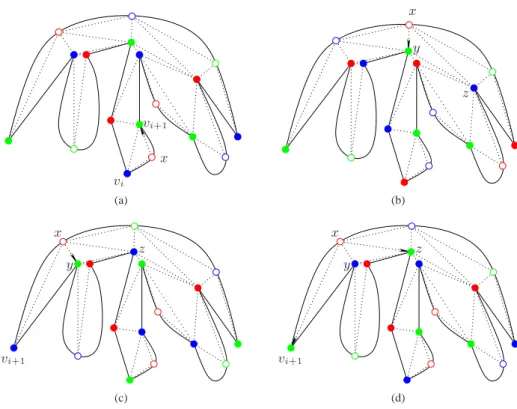
to define a mapping f from KPαto the power set2ΠP ofΠP. Intuitively, f maps a vertex x in KPα
to all the neighboring vertices of x inT ( ˜P) that belong to ΠP. We are going to give a more precise
1. x is an auxiliary vertex added to an empty room ri (see Fig. 10(a)). Then x is one of the
vertices of the constrained triangle vivi+1x contained inside ri. One of vi, vi+1 must be a
vertex inΠP, say vi+1. Then we set f(x) = {vi+1}.
2. x is an auxiliary vertex added to a non-empty room ri. Consider the following subcases:
(a) x is not the last auxiliary vertex on ai, as we walk along aiin the counterclockwise sense
(see Fig. 10(b)). Then x is incident to a single triangle inT ( ˜P) the other two vertices of
which are vertices in P . Let y and z be these other two vertices. One of y and z has to be a green vertex, say y. Then we set f(x) = {y}.
(b) x is the last auxiliary vertex on aias we walk along ai in the counterclockwise sense
(see Figs. 10(c) and 10(d)). Then x is incident to a boundary crescent triangle and an upper crescent triangle. Let xvi+1y be the boundary crescent triangle and xyz the upper
crescent triangle. Clearly, all three vertices vi+1, y and z are vertices of P . If y ∈ ΠP
(this is the case in Fig. 10(c)), then we set f(x) = {y}. Otherwise (this is the case in Fig.
10(d)), both vi+1and z have to be green vertices, in which case we set f(x) = {vi+1, z}.
Now define the set GP = KP∪
³ S
x∈KP αf(x)
´
. We claim that GP is a guarding set for P .
Lemma 6 The set GP = KP ∪
³ S
x∈KP αf(x)
´
is a guarding set for P .
Proof. Let us consider the triangulationT ( ˜P) of ˜P . The regions in Pα are sectors defined by
a curvilinear arc, which is a subarc of an edge of P and the corresponding chord connecting the endpoints of this subarc. Let us consider the set of triangles inT ( ˜P) and the set S(P ) of sectors in Pα. To show that GP is a guarding set for P , it suffices show that every triangle inT ( ˜P) and every
sector inS(P ) is guarded by at least one vertex in GP.
If T is a triangle inT ( ˜P) that is defined over vertices of P , one of its vertices is colored red and
belongs to KP ⊆ GP. Hence, T is guarded.
Consider now a triangle T that is defined inside an empty room ri. If the auxiliary vertex of T
is not red, then one of the two endpoints of aihas to be red, and thus it belongs to GP. Hence both
T and the two sectors adjacent to it in riare guarded. If the auxiliary vertex is red, then one of the
other two vertices of T is green and belongs to GP; again, T is guarded.
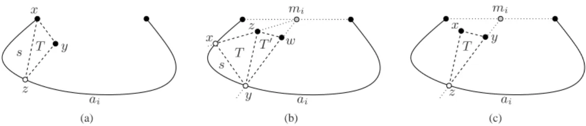
Suppose now that T is a boundary crescent triangle, and let s be the sector adjacent to it (consult Fig. 11(a)). Let x be the endpoint of aicontained in T , y be the second point of T that belongs to P
and z the point in Pα. Note that all three vertices guard the sector s. If x (resp., y) is a red vertex it
will also be a vertex in GP. Hence, in this case both T and s are guarded by x (resp., y). If z is the
red vertex in T , either x or y has to be a green vertex. Hence either x or y will be in GP, and thus
again both T and s will be guarded.
If T is a lower crescent triangle, let s be the sector adjacent to it (consult Fig. 11(b)). Let x, y be the endpoints of the chord of s on ai and let z be the point of P in T . Let us also assume we
encounter x and y in that order as we walk along aiin the counterclockwise sense, which implies
x vi vi+1 (a) x y z (b) x y z vi+1 (c) x y z vi+1 (d)
Figure 10: The three cases in the definition of the mapping f . Case (a): x is a auxiliary vertex in an empty room. Case (b): x is an auxiliary vertex in a non-empty room and is not the last auxiliary vertex added on the curvilinear arc. Cases (c) and (d): x is the last auxiliary vertex added on the curvilinear arc of a non-empty room (in (c) only one of its neighbors in P is green, whereas in (d) two of its neighbors in P are green).
incident to the edge yz, and let w be the third vertex of T′, beyond y and z. It is interesting to note that all four vertices x, y, z and w guard T , T′ and s. Moreover, x and w have to be of the same color. In order to show that T and s are guarded by GP, it suffices to show that one of x, y, z and w
belongs to GP. Consider the following cases:
1. z is a red vertex. Since z∈ KP, we get that z∈ GP.
2. x is a red vertex. But then w is also a red vertex. Since w∈ KP, we conclude that w belongs
to GP as well.
3. y is a red vertex. Then either z is a green vertex or both x and w are green vertices. If z is a green vertex, then{z} ⊆ f (y), which implies that z ∈ GP. If z is a blue vertex, then both x
x y z s T ai (a) x y z w s T T′ ai mi (b) x y z T ai mi (c)
Figure 11: Three of the five cases in the proof of Lemma 6: (a) the triangle T is a boundary crescent triangle; (b) the triangle T is a lower crescent triangle; (c) the triangle T is an upper crescent triangle.
Finally, consider the case that T is an upper crescent triangle, let x and y be the vertices of P in
T and let z be the vertex of T in Pα(consult Fig. 11(c)). Let us also assume that z is the intersection
of the line ymi with ai. To show that T is guarded by GP, it suffices to show that one of x and y
belongs to GP. Consider the following cases:
1. x is red vertex. Since x∈ KPwe have that x∈ GP.
2. y is red vertex. Since y ∈ KP we have that y∈ GP.
3. z is a red vertex. If x is a green vertex, then{x} ⊆ f (z). Hence x ∈ GP. If x is blue vertex,
then y has to be a green vertex, and{y} ⊆ f (z). Therefore, y ∈ GP. 2
Since f(x) ⊆ ΠP for every x in KPαwe get thatS
x∈KP αf(x) ⊆ ΠP. But this, in turn implies
that GP ⊆ KP∪ ΠP. Since KP andΠPare the two sets of smallest cardinality among KP,ΠP and
MP, we can easily verify that|KP| + |ΠP| ≤ ⌊2n3⌋. Hence, |GP| ≤ |KP| + |ΠP| ≤ ⌊2n3⌋, which
yields the following theorem.
Theorem 7 Let P be a piecewise-convex polygon with n≥ 2 vertices. P can be guarded with at
most⌊2n
3⌋ vertex guards.
We close this subsection by making two remarks:
Remark 1 The bound on the size of the vertex guarding set in Theorem 7 is tight: our algorithm will produce a vertex guarding set of size exactly⌊2n3⌋when applied to the piecewise-convex polygon of Fig. 8 or the crescent-like piecewise-convex polygon of Fig. 15.
Remark 2 When the input to our algorithm is a linear polygon all rooms are degenerate; conse-quently, no auxiliary vertices are created, and the guarding set computed corresponds to the set of colored vertices of smallest cardinality, hence producing a vertex guarding set of size at most
⌊n
3⌋. In that respect, it can be considered as a generalization of Fisk’s algorithm [18] to the class of
3.4
Time and space complexity
In this section we will show how to compute a vertex guarding set GP, of size at most⌊2n3⌋, for P ,
in O(n log n) time and O(n) space. The algorithm presented at the beginning of this section consists
of four phases:
1. The computation of the polygonal approximation ˜P of P .
2. The computation of the constrained triangulationT ( ˜P) of ˜P .
3. The computation of a guarding set GP˜for ˜P .
4. The computation of a guarding set GP for P from the guarding set GP˜.
Step 2 of the algorithm presented above can be done in O(T (n)) time and O(n) space, where T(n) is the time complexity of any O(n log n) polygon triangulation algorithm: we need linear time
and space to create the constrained triangles ofT ( ˜P), whereas the subpolygons created after the
introduction of the constrained triangles may be triangulated in O(T (n)) time and linear space.
Step 3 of the algorithm takes also linear time and space with respect to the size of the polygon
˜
P . By Corollary 4,| ˜P| ≤ 3n, which implies that the guarding set GP˜ can be computed in O(n)
time and space.
Step 4 also requires O(n) time. Computing GP from GP˜ requires determining for each vertex
v of KPα all the vertices ofΠP adjacent to it. This takes time proportional to the degree deg(v)
of v inT ( ˜P), i.e., a total ofP
v∈KP αdeg(v) = O(| ˜P|) = O(n) time. The space requirements for
performing Step 4 is O(n).
To complete our time and space complexity analysis, we need to show how to compute the polygonal approximation ˜P of P in O(n log n) time and linear space. In order to compute the
polygonal approximation ˜P or P , it suffices to compute for each room ri the set of vertices Ci∗.
If Ci∗ = ∅, then ri is empty, otherwise we have the set of vertices we wanted. From Ci∗ we can
compute the points wi,kand the linear polygon ˜P in O(n) time and space.
The underlying idea is to split P into y-monotone piecewise-convex subpolygons. For each room riwithin each such y-monotone subpolygon, corresponding to a convex arc aiwith endpoints
viand vi+1, we will then compute the corresponding set Ci∗. This will be done by first computing
a subset Si of the set Ri of the points inside the room ri, such that Si ⊇ Ci∗, and then apply an
optimal time and space convex hull algorithm to the set Si∪ {vi, vi+1} in order to compute Ci, and
subsequently from that Ci∗. In the discussion that follows, we assume that for each convex arc aiof
P we associate a set Si, which is initialized to be the empty set. The sets Siwill be progressively
filled with vertices of P , so that in the end they fulfill the containment property mentioned above. Splitting P into y-monotone piecewise-convex subpolygons can be done in two steps:
1. First we need to split each convex arc ai into y-monotone pieces. Let P′ be the
piecewise-convex polygon we get by introducing the y-extremal points for each ai. Since each aican
yield up to three y-monotone convex pieces, we conclude that|P′| ≤ 3n. Obviously splitting
the convex arcs aiinto y-monotone pieces takes O(n) time and space. A vertex added to split
Q1 Q2 Q3 Q4 Q5 Q6 Q7 Q8 Q9 Q10
Figure 12: Decomposition of a piecewise-convex polygon into ten y-monotone subpolygons. The white points are added extremal vertices that have been added in order to split non-y-monotone arcs to y-monotone pieces. The bridges are shown as dashed segments.
2. Second, we need to apply the standard algorithm for computing y-monotone subpolygons out of a linear polygon to P′(cf. [23] or [12]). The algorithm in [23] (or [12]) is valid not only for line segments, but also for piecewise-convex polygons consisting of y-monotone arcs (such as
P′). Since|P′| ≤ 3n, we conclude that computing the y-monotone subpolygons of P′ takes
O(n log n) time and requires O(n) space.
Note that a non-split arc of P belongs to exactly one y-monotone subpolygon. y-monotone pieces of a split arc of P may belong to at most three y-monotone subpolygons (see Fig. 12).
At the beginning of our algorithm we associate to each arc aiof P a set of vertices Si, which is
initialized to the empty set. Suppose now that we have a y-monotone polygon Q. The edges of Q are either convex arcs of P , or pieces of convex arcs of P , or line segments between mutually visible vertices of P , added in order to form the y-monotone subpolygons of P ; we call these line segments bridges (see Fig. 12). For each non-bridge edge eiof Q, we want to compute the set Ci∗. This can be
done by sweeping Q in the negative y-direction (i.e., by moving the sweep line from+∞ to −∞).
The events of the sweep correspond to the y coordinates of the vertices of Q, which are all known before-hand and can be put in a decreasing sorted list. The first event of the sweep corresponds to the top-most vertex of Q: since Q consists of y-monotone convex arcs, the y-maximal point of Q is necessarily a vertex. The last event of the sweep corresponds to the bottom-most vertex of Q, which is also the y-minimal point of Q. We distinguish between four different types of events:
1. the first event: corresponds to the top-most vertex of Q, 2. the last event: corresponds to the bottom-most vertex of Q,
3. a left event: corresponds to a vertex of the left y-monotone chain of Q, and 4. a right event: corresponds to a vertex of the right y-monotone chain of Q.
Our sweep algorithm proceeds as follows. Let ℓ be the sweep line parallel to the x-axis at some y. For each y in between the y-maximal and y-minimal values of Q, ℓ intersects Q at two points which belong to either a left edge el (i.e., an edge on the left y-monotone chain of Q) or is a left vertex
vl(i.e., a vertex on the left y-monotone chain of Q), and either a right edge er(i.e., an arc on the
right y-monotone chain of Q) or a right vertex vr (i.e., a vertex on the right y-monotone chain of
Q). We are going to associate the current left edge elat position y to a point set SLand the current
right edge at position y to a point set SR. If the edge el(resp., er) is a non-bridge edge, the set SL
(resp., SR) will contain vertices of Q that are inside the room of the convex arc of P corresponding
el(resp., er).
When the y-maximal vertex vmax is encountered, i.e., during the first event, we initialize SL
and SR to be the empty set. When a left event is encountered due a vertex v, let el,upbe the left
edge above v and el,downbe the left edge below v and let erbe the current right edge (i.e., the right
edge at the y-position of v). If el,upis an non-bridge edge, and aiis the corresponding convex arc
of P , we augment the set Siby the vertices in SL. Then, irrespectively of whether or not el,upis
a bridge edge, we re-initialize SL to be the empty set. Finally, if eris a non-bridge edge, and ak
is the corresponding convex arc in P , we check if v is inside the room rk or lies in the interior of
the chord of rk; if this is the case we add v to SR. When a right event is encountered our sweep
algorithm behaves symmetrically. If the right event is due to a vertex v, let er,upbe right edge of Q
above v and er,downbe the right edge of Q below v and let elbe the current left edge of Q. If el,up
is a non-bridge edge, and ai is the corresponding convex arc of P , we augment Si by the vertices
in SR. Then, irrespectively of whether or not er,upis a bridge edge or not, we re-initialize SRto be
the empty set. Finally, If elis a non-bridge edge, and akis the corresponding convex arc of P , we
check if v is inside the room rkor lies in the interior of the chord of rk; if this is the case we add v
to SL. When the last event is encountered due to the y-minimal vertex vmin, let eland erbe the left
and right edges of Q above vmin, respectively. If elis a non-bridge edge, let aibe the corresponding
convex arc in P . In this case we simply augment Siby the vertices in SL. Symmetrically, if eris
a non-bridge edge, let ajbe the corresponding convex arc in P . In this case we simply augment Sj
by the vertices in SR.
We claim that our sweep-line algorithm computes a set Sisuch that Si⊇ Ci∗. To prove this we
need the following intermediate result:
Lemma 8 Given a non-empty room riof P , with aithe corresponding convex arc, the vertices of the
set Ci∗belong to the y-monotone subpolygons of P′computed via the algorithm in [23] (or [12]), which either contain the entire arc aior y-monotone pieces of ai.
Proof. Let ribe a non-empty room, aithe corresponding convex arc and let u be a vertex of P in Ci∗
that is not a vertex of any of the y-monotone subpolygons of P′(computed by the algorithm in [23] or [12]) that contain either the entire arc aior y-monotone pieces of ai. Let vmax(resp., vmin) be the
vertex of P of maximum (resp., minimum) y-coordinate in Ci (ties are broken lexicographically).
vi vi+1 ai ℓu ℓ+ ℓ− u u′ u+ u− w+ s (a) vi vi+1 ai ℓu ℓ+ ℓ− u u′ u+ u− w+ w− s (b) vi vi+1 ai ℓu u u′ w+ w− v′ max (c) Figure 13: Proof of Lemma 8. (a) The case u∈ C∗
i \ {vmin, vmax}, with w+ ∈ s. (b) The case
u∈ C∗
i \ {vmin, vmax}, with w+, w−6∈ s. (c) The case u ≡ vmax.
1. u∈ C∗
i \ {vmin, vmax}. In this case u will be a vertex in either the left y-monotone chain of
Cior a vertex in the right y-monotone chain of Ci. Without loss of generality we can assume
that u is a vertex in the right y-monotone chain of Ci(see Figs. 13(a) and 13(b)). Let u′be the
intersection of ℓuwith ai. Let Q (resp., Q′) be the y-monotone subpolygon of P′that contains
u (resp., u′); by our assumption Q6= Q′. Finally, let u
+(resp., u−) be the vertex of Ciabove
(resp., below) u in the right y-monotone chain of Ci.
The line segment uu′ cannot intersect any edges of P , since this would contradict the fact that u ∈ C∗
i. Similarly, uu′ cannot contain any vertices of P′: if v is a vertex of P in the
interior of uu′, u would be inside the triangle vu+u−, which contradicts the fact that u∈ Ci∗,
whereas if v is a vertex of P′\ P in the interior of uu′, P would not be locally convex at
v, a contradiction with the fact that P is a piecewise-convex polygon. As a result, and since Q6= Q′, there exists a bridge edge e intersecting uu′. Let w
+, w−be the two endpoints of e
in P′, where w+lies above the line ℓuand w−lies below the line ℓu. In fact neither w+nor
w− can be a vertex in P′\ P , since the algorithm in [23] (or [12]) will connect a vertex in
P′\ P inside a room rk with either the y-maximal or the y-minimal vertex of Ck only. Let
ℓ+(resp., ℓ−) be the line passing through the vertices u and u+(resp., u and u−). Finally, let
s be the sector delimited by the lines ℓ+, ℓ− and ai. Now, if w+lies inside s, then u will be
inside the triangle w+u+u−(see Fig. 13(a)). Analogously, if w−lies inside s, then u will be
inside the triangle w−u+u−. In both cases we get a contradiction with the fact that u∈ Ci∗.
If neither w+ nor w− lie inside s, then both w+ and w− have to be vertices inside ri, and
moreover u will lie inside the convex quadrilateral w+u+u−w−; again this contradicts the
fact that u∈ C∗
i (see Fig. 13(b)).
2. u ≡ vmax. By the maximality of the y-coordinate of u in Ci, we have that the y-coordinate
of u is larger than or equal to the y-coordinates of both vi and vi+1. Therefore, the line ℓu
intersects the arc ai exactly twice, and, moreover, ai has a y-maximal vertex of P′ \ P in
ai that lies to the right of u, and let Q (resp., Q′) be the y-monotone subpolygon of P′ that
contains u (resp., u′). By assumption Q6= Q′, which implies that there exists a bridge edge e
intersecting the line segment uu′. Notice, that, as in the case u∈ C∗
i \ {vmin, vmax}, the line
segment uu′ cannot intersect any edges of P , or cannot contain any vertex v of P′\ P ; the
former would contradict the fact that u∈ C∗
i, whereas as the latter would contradict the fact
that P is piecewise-convex. Furthermore, uu′ cannot contain vertices of P since this would contradict the maximality of the y-coordinate of u in Ci.
Let w+and w−be the endpoints of e above and below ℓu, respectively. Notice that e cannot
have vmax′ as endpoint, since the only bridge edge that has v′maxas endpoint is the bridge edge
vmax′ u. But then w+must be a vertex of P lying inside ri; this contradicts the maximality of
the y-coordinate of u among the vertices in Ci.
3. u≡ vmin. This case is entirely symmetric to the case u≡ vmax. 2
An immediate corollary of the above lemma is the following:
Corollary 9 For each convex arc aiof P , the set Si computed by the sweep algorithm described
above is a superset of the set Ci∗.
Let us now analyze the time and space complexity of Step 1 of the algorithm sketched at the beginning of this subsection. Computing the polygonal approximation ˜P of P requires subdividing P into y-monotone subpolygons. This subdivision takes O(n log n) time and O(n) space. Once we
have the subdivision of P into y-monotone subpolygons we need to compute the sets Sifor each
convex arc ai of P . The sets Si can be implemented as red-black trees. Inserting an element in
some Sitakes O(log n) time. During the course of our algorithm we perform only insertions on the
Si’s. A vertex v of P is inserted at most deg(v) times in some Si, where deg(v) is the degree of
v in the y-monotone decomposition of P . Since the sum of the degrees of the vertices of P in the y-monotone decomposition of P is O(n), we conclude that the total size of the Si’s is O(n) and
that we perform O(n) insertions on the Si’s. Therefore we need O(n log n) time and O(n) space
to compute the Si’s. Finally, sincePni=1|Si| = O(n), the sets Ci∗can also be computed in total
O(n log n) time and O(n) space. The analysis above thus yields the following:
Theorem 10 Let P be a piecewise-convex polygon with n≥ 2 vertices. We can compute a guarding
set for P of size at most⌊2n3⌋ in O(n log n) time and O(n) space.
3.5
The lower bound construction
In this section we are going to present a piecewise-convex polygon which requires a minimum of
⌊4n
7⌋ − 1 vertex guards in order to be guarded.
Let us first consider the windmill-like piecewise-convex polygon W with seven vertices of Fig. 14(a), a detail of which is shown in Fig. 14(b). The double ear defined by the vertices v3, v4 and
v5and the convex arcs a3 and a4is constructed in such a way so that neither v3nor v5can guard
v4v5 (resp., v3v4) twice. Note that both a3and a4 intersect the line mv4 only at v4, where m is
the midpoint of the line segment v3v5. The double ear defined by the vertices v5, v6and v7and the
convex arcs a5and a6is constructed in an analogous way. Moreover, the vertices v1, v2, v4and v6
are placed in such a way so that they do not (collectively) guard the interior of the triangle v3v5v7
(for example the lengths of the edges v1v7and v2v3are considered to be big enough, so that v2does
not see too much of the triangle v3v5v7). As a result of this construction, W cannot be guarded by
two vertex guards, but can be guarded with three. There are actually only five possible guarding triplets:{v3, v4, v6}, {v3, v5, v6}, {v3, v5, v7}, {v4, v5, v7} and {v4, v6, v7}. Any guarding set that
contains either v1 or v2 has cardinality at least four. The vertices v1and v2will be referred to as
base vertices.
Consider now the crescent-like polygon C with n vertices of Fig. 15. The vertices of C are in strictly convex position. This fact has the following implication: if vi, vi+1, vi+2and vi+3are four
consecutive vertices of C, and u is the point of intersection of the lines vivi+1and vi+2vi+3, then
the triangle vi+1uvi+2is guarded if and only if either vi+1or vi+2is in the guarding set of C. As a
result, it is easy to see that C cannot be guarded with less than⌊n
2⌋ vertices, since in this case there
will be at least one edge both endpoints of which would not be in the guarding set for C.
In order to construct the piecewise-convex polygon that gives us the lower bound mentioned at the beginning of this section, we are going to merge several copies of W with C. More precisely, consider the piecewise-convex polygon P of Fig. 16 with n= 7k vertices. It consists of copies of
the polygon W merged with C at every other linear edge of C, through the base points of the W ’s. In order to guard any of the windmill-like subpolygons, we need at least three vertices per such polygon, none which can be a base point. This gives a total of3k vertices. On the other hand, in
order to guard the crescent-like part of P we need at least k− 1 guards among the base points. To
v1 v2 v3 v4 v5 v6 v7 (a) v3 v4 v5 m a3 a4 (b)
Figure 14: The windmill-like piecewise-convex polygon W that requires at least three vertex guards in order to be guarded. The only triplets of guards that guard W are{v3, v4, v6}, {v3, v5, v6},
vi
vi+1
vi+2 vi+3
u
Figure 15: The crescent-like piecewise-convex polygon C, that requires a guarding set of at least
⌊n
2⌋ vertex guards.
Figure 16: The lower bound construction.
see that, notice that there are k− 1 linear segments connecting base points; if we were to use less
than k− 1 guards, we would have at least one such line segment e, both endpoints of which would
not participate in the guarding set of G. But then, as in the case of C, there would be a triangle, adjacent to e, which would not be guarded. Therefore, in order to guard P we need a minimum of
Theorem 11 There exists a family of piecewise-convex polygons with n vertices any vertex guarding
set of which has cardinality at least⌊4n 7 ⌋ − 1.
4
Monotone piecewise-convex polygons
In this section we focus on the subclass of piecewise-convex polygons that are monotone. Let us recall the definition of monotone polygons from Section 1: a curvilinear polygon P is called monotone if there exists a line L such that any line L⊥ perpendicular to L intersects P at most twice.
In the case of linear polygons monotonicity does not yield better bounds on the worst case num-ber of point or vertex guards needed in order to guard the polygon. In both cases, monotone or possi-bly non-monotone linear polygons,⌊n
3⌋ point or vertex guards are always sufficient and sometimes
necessary. In the context of piecewise-convex polygons the situation is different. Unlike general (i.e., not necessarily monotone) piecewise-convex polygons, which require at least⌊4n
7 ⌋ − 1 vertex
guards and can always be guarded with⌊2n
3 ⌋ vertex guards, monotone piecewise-convex polygons
can always be guarded with⌊n
2⌋ + 1 vertex or ⌊ n
2⌋ point guards. These bounds are tight, since there
exist monotone piecewise-convex polygons that require that many vertex (see Figs. 18 and 19) or point guards (see Fig. 20). This section is devoted to the presentation of these tight bounds.
Vertex guards. Let us consider a monotone piecewise-convex polygon P , and let us assume without loss of generality that P is monotone with respect to the x-axis (see also Fig. 17). Let uj,
1 ≤ j ≤ n, be the j-th vertex of P when considered in the list of vertices sorted with respect to their x-coordinate (ties are broken lexicographically). Let also u0 (resp., un+1) be the left-most (resp.,
right-most) point of P . Let ℓj,0 ≤ j ≤ n + 1 be the vertical line passing through the point uj of
P , and letL = {ℓ0, ℓ1, ℓ2, . . . , ℓn+1} be the collection of these lines. An immediate consequence of
the fact that P is monotone and piecewise-convex is the following corollary:
Corollary 12 The collection of lines L decomposes the interior of P into at most n + 1 convex
regions κj, j= 0, . . . , n, that are free of vertices or edges of P .
In addition to the fact that the region κj,1 ≤ j ≤ n − 1, is convex, κjhas on its boundary both
vertices ujand uj+1. This immediately implies that both ujand uj+1see the entire region κj. As
far as κ0and κnare concerned, they have u1and unon their boundary, respectively. As a result, u1
sees κ0, whereas un sees κn. Hence, in order to guard P it suffices to take every other vertex uj,
starting from u1, plus un(if not already taken). The set G= {u2m−1,1 ≤ m ≤ ⌊n2⌋} ∪ {un} is,
thus, a vertex guarding set for P of size⌊n 2⌋ + 1.
A line L with respect to which P is monotone can be computed in O(n) time if it exists [13].
Given L, we can compute the vertex guarding set G for P in O(n) time and O(n) space: project the
vertices of P on L and merge the two sorted (with respect to their ordering on L) lists of vertices in the upper and lower chain of P ; then report every other vertex in the merged sorted list starting from the first vertex, plus the last vertex of P , if it has not already been reported.
The polygons M1and M2yielding the lower bound are shown in Figs. 18 and 19. M1has an odd
u0 u ′ 2 u10 v1 v2 v3 v4 v5 v6 v7 v8 v9
Figure 17: A monotone piecewise-convex polygon P with n= 9 vertices and its vertical
decompo-sition into four-sided convex slabs. The points u0and u10are the left-most and right-most points of
P ; u′
2is the projection of u2 ≡ v9, along ℓ2, on the opposite chain of P . P can be either guarded
with: (1)⌊n
2⌋ + 1 = 5 vertices, namely the vertex set {u1, u3, u5, u7, u9} ≡ {v1, v8, v3, v7, v6}, or
⌊n
2⌋ = 4 points, namely the point set {u ′
2, u4, u6, u8} ≡ {u′2, v2, v4, v5}.
Figure 18: A monotone piecewise-convex polygon M1with an odd number of vertices that requires
⌊n
2⌋ + 1 vertex guards in order to be guarded: the shaded regions require that at least one of the two
endpoints of the bottom-most edge of the polygon to be in the guarding set.
guarding set for M1(resp., M2). Let us first consider M1(see Fig. 18). Notice that each prong of
M1is fully guarded by either of its two endpoints; the other vertices of M1can only partially guard
the prongs that they are not adjacent to. Moreover, the shaded regions of M1can only be guarded
by u1or un. Suppose, now, we can guard M1with less than⌊n2⌋ + 1 vertex guards. Then either two
consecutive vertices ui and ui+1 of M1,1 ≤ i ≤ n − 1, will not belong to G1, or u1and un will
not belong to G1. In the former case, the prong that has uiand ui+1as endpoints is only partially
guarded by the vertices in G1, a contradiction. In the latter case, the shaded regions of M1are not