Length-of-day and space-geodetic determination of the Earth's variable gravity field

HAL Id: hal-00176445

https://hal.archives-ouvertes.fr/hal-00176445

HAL is a multi-disciplinary open access

archive for the deposit and dissemination of sci-entific research documents, whether they are pub-lished or not. The documents may come from teaching and research institutions in France or abroad, or from public or private research centers.

L’archive ouverte pluridisciplinaire HAL, est destinée au dépôt et à la diffusion de documents scientifiques de niveau recherche, publiés ou non, émanant des établissements d’enseignement et de recherche français ou étrangers, des laboratoires publics ou privés.

Earth’s variable gravity field

G. Bourda

To cite this version:

G. Bourda. Length-of-day and space-geodetic determination of the Earth’s variable gravity field. Journal of Geodesy, Springer Verlag, 2008, 82 (4-5), pp.295-305. �10.1007/S00190-007-0180-Y�. �hal-00176445�

G. Bourda

Length-of-day and space-geodetic determination of the Earth’s

variable gravity field

Received: 17/02/2007 / Accepted: 27/07/2007

Abstract The temporal variations of the Earth’s gravity field,

nowadays routinely determined from Satellite Laser Rang-ing (SLR) and GRACE, are related to changes in the Earth’s rotation rate through the Earth’s inertia tensor. We study this connection from actual data by comparing the traditional length-of-day (LOD) measurements provided by the Interna-tional Earth Rotation and reference systems Service (IERS) to the variations of the degree-2 and order-0 Stokes coeffi-cient of the gravity field determined from fitting the orbits of the LAGEOS 1 and 2 satellites since 1985. The two se-ries show a good correlation (0.62) and similar annual and semi-annual signals, indicating that the gravity-field-derived LOD is valuable. Our analysis also provides evidence for ad-ditional signals common to both series, especially at a period near 120 days, which could be due to hydrological effects.

Keywords Earth rotation · length-of-day · gravity field · C20· satellite laser ranging · LAGEOS

1 Introduction

Studies of the Earth’s rotation are aimed at modeling its vari-ations as precisely as possible, on the basis of geodetic mea-surements and geophysical models. Offsets with respect to a uniform rotation around a fixed axis or an analytical model are described by the Earth’s Orientation Parameters (EOPs). These parameters consist of the polar motion coordinates, the celestial pole offsets and the Earth’s rotation rate.

The Length-of-day (LOD) is used to characterize the vari-ability of the Earth’s rotation rate. The LOD variations are due to gravitational effects from external bodies (i.e., luni-solar tides; Defraigne and Smith 1999), but also originate from geophysical deformations occuring in various layers

G. Bourda

Centre National de Recherche Scientifique (CNRS), Observatoire Aquitain des Sciences de l’Univers (OASU), Unit´e Mixte de Recherche 5804, Universit´e Bordeaux 1, 33270 Floirac, France

E-mail: geraldine.bourda@obs.u-bordeaux1.fr

of the Earth (i.e., atmosphere, oceans, hydrosphere, mantle, core; Barnes et al. 1983; Gross et al. 2004).

Each of the geophysical contributions to the LOD varia-tions is traditionally divided into (i) a motion term, and (ii) a

massterm (Barnes et al. 1983; Eubanks 1993). This comes from the Euler-Liouville equations for the angular momen-tum conservation (Munk and McDonald 1960). For exam-ple, the atmosphere acts on the LOD variations through the effect of the winds (motion term) and the effect of the at-mospheric pressure onto the crust (mass term). The motion contribution to the LOD variations may be modeled from the data gathered by the Special Bureau for the Atmosphere (SBA) and the Special Bureau for the Oceans (SBO), de-pending on the Global Geophysical Fluid Center (GGFC) from the International Earth Rotation and reference systems Service (IERS).

The mass contribution is due to dynamical processes in the Earth system that affect the mass distribution (it is equiv-alent to gravitational effects). The Earth’s mass distribution, described by the inertia tensor, also acts directly on the Earth’s gravity field, therefore implying a relationship be-tween the LOD and gravity field variations (Lambeck 1988; Chao 1994; Gross 2001).

The purpose of the study presented here is the investi-gation of this relationship by comparison of standard LOD measurements with gravity field data, in order to determine if the latter could be useful to supplement classical LOD es-timates. The motivation also originates in the requirement to prepare for the ambitious project GGOS (Global Geode-tic Observing System) of the IAG (International Association of Geodesy), which ultimate goal is a consistent and inte-grated treatment of the three pillars of geodesy (Rummel et al. 2005): (1) the geometry and deformation of the Earth’s surface, (2) the Earth’s rotation and orientation, and (3) the Earth’s gravity field and its temporal variations.

LOD data used in geodesy, geophysics or astronomy come from the combination of the results from various geode-tic observation techniques. Very Long Baseline Interferome-try (VLBI) is the primary technique, which permits determi-nation of all the EOPs (Schuh and Schmitz-H¨ubsch 2000;

Schl¨uter and Behrend 2007). Global Positionning System (GPS) and Satellite Laser Ranging (SLR) allow to obtain po-lar motion coordinates and LOD (Lichten at al. 1992; Tapley et al. 1985), while Doppler Orbitography by Radioposition-ing Integrated on Satellite (DORIS) and Lunar Laser Rang-ing (LLR) may be selectively used for such determinations (Gambis 2006; Dickey and Williams 1983).

Gravity field data, represented in the form of Stokes co-efficients, are nowadays routinely obtained by precise or-bitography of geodetic satellites (for example based on SLR measurements; Nerem et al. 1993; Tapley et al. 1993; Bian-cale et al. 2000) or dedicated space gravimetric missions like CHAMP (CHAllenging Minisatellite Payload; Reigber et al. 2002) or GRACE (Gravity Recovery And Climate Experi-ment; Reigber et al. 2005).

Several studies have already investigated (i) the long-term variation (Yoder et al. 1983; Rubincam 1984; Cheng et al. 1997; Cox and Chao 2002; Dickey et al. 2002) and (ii) the seasonal variations (Chao and Au 1991; Chao and Eanes 1995; Chao and Gross 1987; Gegout and Cazenave 1993; Cheng and Tapley 1999) of the Stokes coefficients, especially the degree-2 and order-0 coefficient C20, which characterizes the gravitational oblateness of the Earth.

Variations of the gravity field have also been investigated by using EOP data (Chen et al. 2000; Chen and Wilson 2003; Chen et al. 2005). Bourda (2004, 2005) and Yan et al. (2006) instead derived LOD and polar motion from temporal series of the C20, C21and S21Stokes coefficients.

This study is focused on the LOD parameter. For this purpose, we compare the LOD series derived from the C20 variations (hereafter referred to as geodetic data) to the stan-dard LOD series derived mainly from VLBI, GPS and SLR (hereafter referred to as astrometric data). These two types of data are not entirely equivalent: (1) the astrometric data are relative to the crust of the Earth, whereas the geodetic

data are relative to the entire Earth measured from space (Chao 2005); (2) the astrometric data are sensitive to all geophysical processes inducing variations of the LOD (i.e., the mass and motion terms), whereas the geodetic data are only sensitive to gravitational effects into the Earth system (i.e., the mass terms). These differences will be accounted for when comparing the two LOD series.

In the following, we first detail the equations linking the LOD and the C20Stokes coefficient (Lambeck 1988; Gross 2001; Chen et al. 2005). Then, we present the data used for our study and the processing to determine the corresponding LOD variations. The standard LOD data used for compar-ison come from the IERS and results from a combination of mainly VLBI, GPS and SLR measurements. The grav-ity field data were obtained by the GRGS/CNES (Groupe de Recherche de G´eod´esie Spatiale/Centre National d’Etudes Spatiales, Toulouse, France) on the basis of SLR orbitogra-phy (LAGEOS I and II gravity field data). We could have used GRACE data, but the C20 Stokes coefficient series de-rived from GRACE measurements are known to show a long-term drift and are thus less accurate than those from SLR

(personal communication from Lemoine 2004). In addition, SLR data cover a much longer period than GRACE data (20 years for SLR against 5 years for GRACE), which is more interesting for comparison of LOD measurements.

We compare the LOD mass terms obtained from both se-ries by determining the correlation coefficient between the two series and by estimating annual and semi-annual signals with a Fourier analysis. We also investigate the intraseasonal terms that remain in each of the series after this Fourier anal-ysis. Finally, we discuss the consistency of the results and draw further prospects about using gravity field data to sup-plement current LOD measurements.

2 Theory

2.1 Earth’s tensor of inertia

The Earth’s tensor of inertia I, characterizing the mass dis-tribution in the Earth system (i.e., solid Earth, atmosphere, oceans, hydrosphere), is defined in the terrestrial frame (Oxyz) by: I(t) =   I11 I12I13 I12 I22I23 I13 I23I33  (t) (1) with: I11= % y % z(y 2_{+ z}2_{) dM} I12= − % x % yxydM I22= % x % z (x2+ z2) dM I23= − % y % z yzdM (2) I33= % x % y (x2_{+ y}2_{) dM I} 13= − % x % z xzdM where M is the mass of the Earth.

In practice, the Earth is not only considered as an el-lipsoid of rotation but also as a deformable body. For this reason, its tensor of inertia is not diagonal. Then, I may be written as: I(t) =   A 0 0 0 B 0 0 0 C  +   c11c12 c13 c12c22 c23 c13c23 c33  (t) (3)

where A, B and C are the mean principal moments of iner-tia (representing the part of the tensor that is constant with time) and ci j (for i, j = 1, 2, 3) are the products of inertia

(representing the shift to the mean ellipsoidal solid Earth) such that each of the ci j/C is very small.

2.2 Earth’s Gravity Field

The Earth’s gravity field U(r, ! , " ) is traditionally developed into spherical harmonics (Kaula 1966):

U(r, ! , " ) =GM r +#

$

$

where r is the geocentric distance, ! is the geocentric lati-tude and " is the longilati-tude of the determination point; G is the gravitational constant and Re is the mean equatorial

ra-dius of the Earth. Cnmand Snm are the Stokes coefficients,

defined by: Cnm Snm ( =(2 − %0m) MRen (n − m)! (n + m)! % M

rnPnm(sin ! )) cosm"_{sin m"}

(

dM

(5) where(r, ! , " ) are the coordinates of the mass element dM in the terrestrial reference frame(Oxyz), Pnm(sin ! ) are the

Legendre polynomials (Lambeck 1988), and %0m= 1 if m = 0 or %0m_{= 0 if m "= 0. We can notice that in practice, the} nor-malized Stokes coefficients ¯Cnmand ¯Snmare generally used

(Lambeck 1988).

In order to take into account the yielding of the solid Earth as the surface mass is redistributed, a loading coeffi-cient(1 + k#

n) is generally applied into the right hand side

of Eq. (5) (see Chen et al. 2005), then C20 may be further expressed as: C20 = (1 + k2#) 1 2 MRe2 % M r2(3 sin2 ! − 1) dM = (1 + k2#) 1 2 MRe2 % M *3z2 − r2+ dM = (1 + k2#) 1 2 MRe2 % M *2z2 − x2− y2+ dM (6) where k#_{2= −0.301 is the load Love number of degree 2} (Farrel 1972). Finally, after introducing in Eq. (6) the com-ponents of the inertia tensor defined in Eq. (2), one obtains:

C20 = (1 + k2#) 1 2 MRe2[−I 33+ (I11+ I22− I33)] = (1 + k2#) 1 MRe2 , I11+ I22 2 − I33 -, (7)

which relates the C20Stokes coefficient to the inertia tensor.

2.3 Relation between C20variations and the inertia tensor On the basis of Eq. (7), the inertia tensor component I33can be related to the degree-2 and order-0 Stokes coefficient C20 by (Lambeck 1988; Gross 2001): I33(t) =I11+ I22 2 (t) − M Re 2 C20(t) 1+ k# 2 (8) Using the trace of the inertia tensor Tr(I) = I11+ I22+ I33 (i.e., the sum of its diagonal elements), Eq. (8) can be further expressed as: I33(t) =1 3Tr(I)(t) − 2 3 M Re 2C20(t) 1+ k# 2 (9)

Then, from Eq. (3), the product of inertia c33 (i.e., I33− C) can be written: c33(t) =1 3& Tr(I) − 2 3M R 2 e &C20(t) 1+ k# 2 (10) where & Tr(I) is the change in the trace of the Earth’s iner-tia tensor following mass redistribution, and &C20(t) is the corresponding shift in the Stokes coefficient C20.

2.4 Link between LOD and gravity field through the inertia tensor

Assuming that the instantaneous Earth’s rotation vector is given by: −→' = ('1, '2, '3)T _{= ( (m1, m2, 1 + m3)}T_{, where}

( is the nominal mean angular velocity of the Earth and (m1, m2, m3) are small variations with respect to constant ro-tation, the changes & LOD in the length-of-day with respect to the mean length-of-day LODmean can be written

(Lam-beck 1988): −& LOD(t)

LODmean

= m3(t) (11)

where LODmean= 86400 seconds.

The expression for m3 may then be obtained from the Liouville equations, which characterize the rotation of a non rigid Earth, based on the angular momentum conservation (Munk and McDonald 1960):

m3(t) = − 1 Cm( .h3(t) + (1 + k# 2) ( c33(t) / (12) where Cm is the third principal moment of inertia of the

Earth’s mantle, h3 is the axial relative angular momentum of the Earth (corresponding to the motion term) and k#₂ c33 accounts for loading effects in the inertial part of m3 (i.e., in the mass term of m3; see Barnes et al. 1983). In Eq. (12), the effects of external bodies (Sun and Moon) are not con-sidered, because nowadays they are modeled very properly (McCarthy and Petit 2004).

Combining Eqs. (11) and (12), we further obtain: & LOD(t) LODmean = (1 + k#2) c33(t) Cm + h3(t) Cm( (13) Finally, on the basis of Eqs. (10) and (13), we can link & LOD with the C20Stokes coefficient variations through:

& LOD(t) LODmean = − 2 3 Cm M R2e&C20(t) + h3(t) Cm( (14) where it is assumed that & Tr(I) = 0, i.e., the trace of the inertia tensor is constant with time.

This assumption (i.e., & Tr(I) = 0) is true in the case of a closed system (i.e., with no mass loss) such that comprising the entire Earth (solid earth + oceans + atmosphere + hydro-sphere) (see Rochester and Smylie 1974). This was verified

1965 1970 1975 1980 1985 1990 1995 2000 2005 Years -2 -1 0 1 2 3 4 5 V al ue s (m s) IERS C04

Fig. 1 Observed & LOD data (with respect to LODmean= 86400

sec-onds) from the IERS-C04 series.

by Chen et al. (2005), who calculated & Tr(I) from models of atmospheric pressure and terrestrial water storage loads. They conclude that typical annual &C20 variability due to & Tr(I) change is about 10−13, less than 0.1 % of the vari-ations measured by SLR. Neglecting & Tr(I) in Eq. (14) is therefore a reasonable assumption.

3 Data and Processing

3.1 Length-of-day astrometric data

The LOD series used in this study as the basis for the ob-served & LOD is the IERS-C04 series (Gambis 2004), which covers the period 1962-2006 (see http://hpiers.obspm.fr/eop-pc, Fig. 1). As noted above, these measurements refer not only to mass gravitational effects but also to motions into the Earth system.

In order to compare these astrometric data with those obtained from gravity field variations, it is therefore neces-sary to remove the following contributions from the data: (i) zonal tides, (ii) atmospheric winds, and (iii) oceanic cur-rents. Figure 2 summarizes the successive steps to extract the mass term & LODastro from the original IERS-C04

se-ries. The models removed are listed in Table 1 and described in further detail below.

3.1.1 Zonal tide variations

The zonal tidal model removed from the IERS-C04& LOD series is the IERS Conventions 2003 model (Defraigne and Smith 1999). This model covers the period 1962–2006 and the corresponding LOD variations are plotted in Fig. 3.

&LOD astro & zonal winds LOD IERS C04 &LOD Zonal Tides &LOD oceanic currents &LOD Models removed Observed Data

Filters and New sampling

Fig. 2 Diagram explaining the derivation of the astrometric & LOD

mass term-series (i.e., & LODastro) from the original & LOD IERS-C04

data. 1965 1970 1975 1980 1985 1990 1995 2000 2005 Years -1.5 -1 -0.5 0 0.5 1 1.5 V al ue s (m s)

Zonal Tides model (IERS Conventions 2003)

Fig. 3 Zonal tides contribution to & LOD (with respect to LODmean=

86400 seconds) as published in the IERS Conventions 2003 model (McCarthy and Petit 2004; Defraigne and Smith 1999).

3.1.2 Atmospheric Angular Momentum (AAM)

The motion part of the atmospheric& LOD contribution (zonal winds) is defined by:

& LODwinds(t) LODmean

=h3 winds(t)

Cm(

(15) For our study, it has been calculated from the NCEP (Na-tional Centers for Environmental Prediction) reanalysis AAM products for the period 1962–2006 (Fig. 4). These data, in their original form (i.e., as published by the SBA), have a six-hour sampling, but for our analysis we used the series made available by the IERS, which has a 24-hour sampling.

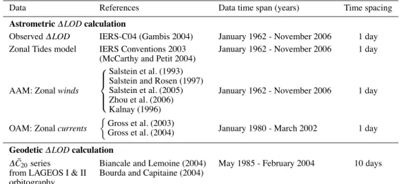
Table 1 Temporal series used in this study for: (1) the astrometric & LOD calculation, and (2) the gravity field C20derived geodetic & LOD (AAM

means Atmospheric Angular Momentum; OAM means Oceanic Angular Momentum).

Data References Data time span (years) Time spacing

Astrometric& LOD calculation

Observed & LOD IERS-C04 (Gambis 2004) January 1962 - November 2006 1 day

Zonal Tides model IERS Conventions 2003 January 1962 - November 2006 1 day

(McCarthy and Petit 2004)

AAM: Zonal winds        Salstein et al. (1993) Salstein and Rosen (1997) Salstein et al. (2005) Zhou et al. (2006) Kalnay (1996)

January 1962 - November 2006 1 day

OAM: Zonal currents ) Gross et al. (2003)

Gross et al. (2004) January 1980 - March 2002 1 day

Geodetic& LOD calculation

& ¯C20series Biancale and Lemoine (2004) May 1985 - February 2004 10 days

from LAGEOS I & II Bourda and Capitaine (2004) orbitography 1965 1970 1975 1980 1985 1990 1995 2000 2005 Years 1 1.5 2 2.5 3 3.5 4 V al ue s (m s)

AAM zonal winds

Fig. 4 Atmospheric angular momentum motion contribution (i.e.,

zonal winds) to& LOD (with respect to LODmean= 86400 seconds).

3.1.3 Oceanic Angular Momentum (OAM)

The motion part of the oceanic & LOD contribution (zonal currents) is defined by:

& LODcurrents(t) LODmean

=h3 currents(t)

Cm(

(16) This effect has been calculated based on OAM products from the SBO (Gross et al. 2003, 2004) for the period 1980–2002 (http://euler.jpl.nasa.gov/sbo/sbo data.html, Fig. 5).

3.1.4 Long-period terms

After removing the zonal tide, AAM and OAM contribu-tions from the original IERS-C04 & LOD series, long-period

1980 1985 1990 1995 2000 Years -0.08 -0.06 -0.04 -0.02 0 0.02 0.04 0.06 0.08 V al ue s (m s)

OAM zonal currents

Fig. 5 Oceanic angular momentum motion contribution (i.e., zonal

currents) to & LOD (with respect to LODmean= 86400 seconds).

terms (i.e., periods of 10 years or more in Fig. 1) still remain into the resulting series. These are due to coupling between the core and the mantle. As pointed out above, such

astro-metric& LOD data are referred to the Earth’s crust, whereas

geodetic& LOD data are referred to the global Earth system. These long-period terms are thus not expected to appear into the gravity-field-derived LOD data. This is the reason why we subtracted these long-period terms from the

astromet-ric& LOD data in an additional processing step. A Vondrak (1977) filter with a half-width period of 1200 days was used for this purpose (this half-width period was aimed at remov-ing the signal with a period longer than 7 years but keepremov-ing intact the seasonal signal).

Finally, in order to compare this series with the

geode-tic & LOD series described in Sect. 3.2 below, we also fil-tered the high-frequency terms and sampled the data

ev-ery 10 days. In order to remove all the periodic terms less than 20 days (i.e., corresponding to the Nyquist period for a 10-day sampling), a Vondrak filter was applied with a half-width period of 50 days. The astrometric & LOD series thus obtained is denoted as & LODastro.

3.2 Gravity field data

Table 1 provides the characteristics of the gravitational data used to derive the geodetic & LOD mass term on the basis of Eq. (14). These data consist of a series of ¯C20fully normal-ized Stokes coefficient estimates (C20=√5 ¯C20) obtained by the GRGS/CNES from fitting the orbits of the LAGEOS I & II satellites over the period 1985-2004 with the software GINS (G´eod´esie par Int´egrations Num´eriques Simultan´ees). GINS is a multi-technique software, that has been devel-oped for about 30 years by the GRGS/CNES in Toulouse (France), initially for analyzing SLR data, and extended at later stages for analysis of GPS, DORIS, LLR and VLBI data (see for example Coulot et al. 2007). Based on such data, GINS is able to fit the orbit of a satellite around the Earth or another body of the solar system and estimate geo-physical parameters (e.g., gravity field coefficients; Biancale et al. 2000; Reigber et al. 2004).

In our case, LAGEOS I and II orbits were derived by fit-ting the SLR observations with orbital models comprising the equations of motion and surface pressure atmospheric forcing. In this calculation, the fully normalized degree-2 and order-0 Stokes coefficient ¯C20 of the gravity field was estimated every 10 days (along with the rest of the degree-2 gravity field coefficients), permitting the determination of the total variations & ¯C20of this coefficient.

As depicted in Fig. 6, the contributions due to solid Earth tides, atmospheric pressure and oceanic tides were further removed from the & ¯C20series (and from the other degree-2 Stokes coefficients) for a more precise gravity field determi-nation by the GRGS. These were calculated based on models for the geopotential from the IERS Conventions 1996 (Mc-Carthy 1996) and using the equations for the ¯C20variations given in Bourda and Capitaine (2004).

The & ¯C20 series delivered by the GRGS/CNES (here-after referred to as ¯C20residualseries) is then free from these geophysical effects. Comparing the gravity-field-derived LOD variations with the astrometric & LOD data requires, however, adding back the ¯C20variations due to atmospheric pressure (see & ¯C20from atmospheric pressure in Fig. 6, re-moved by the GRGS during the determination of the grav-ity field; see also Bourda and Capitaine 2004) to this resid-ual series, because atmospheric mass terms are still included into the & LODastro data. The resulting series (i.e., that

in-cluding residual effects and atmospheric pressure variations) is plotted in Fig. 7 along with the original & ¯C20 total varia-tions (in which the predominant effect comes from the solid Earth tides).

&C total variations (equivalent to observed data)20

solid Earth tides

Models removed during processing by the GRGS/CNES

&C₂₀ &

atm. pressure

C₂₀ &

oceanic tides C₂₀

&LOD geod domain

LOD

&Tr(I)=0 hypothesis

domain Gravity residuals

&C_{20 Data delivered by}

&C₂₀ atm. pressure model added back

**

** the GRGS/CNES

Fig. 6 Diagram explaining the calculation of the geodetic & LOD mass

term-series (& LODgeod) from the original & ¯C20data (** means that the

same atmospheric pressure model for & ¯C20is used during both steps).

1985 1990 1995 2000 Years -1e-09 -5e-10 0 5e-10 1e-09 V al ue s (ra d)

Normalized C20: (residuals + atmospheric pressure) effects Normalized C20: complete variations

Fig. 7 GRGS series from LAGEOS I and II orbitography for the ¯C20

variations. The dashed line plots the & ¯C20total variations, while the

full line plots only the residual effects and atmospheric pressure varia-tions.

From the residual and atmospheric pressure & ¯C20 data, one can now derive the corresponding LOD variations on the basis of Eq. (14). For this calculation, the fundamental constants listed in Table 2 have been used. In an additional processing step, as already done in the case of the

astro-metric& LOD mass term-series (to subtract the core-mantle effects), we applied a Vondrak filter with a half-width pe-riod of 1200 days. This process was aimed at removing the long-period terms (i.e., longer than 10 years), in order to get homogeneous signal for comparing both & LOD mass term-series. The geodetic & LOD mass term-series obtained at this

Table 2 Fundamental constants used for the calculation of & LODgeod

(McCarthy and Petit 2004; Barnes et al. 1983).

Parameter Value

Constant of gravitation G 6.673_{× 10}−11

m3_kg−1_s−1

Geocentric gravitational GM 3.986004418× 1014

constant m3_s−1

Mass of the Earth M=GM

G 5.9736 × 10

24_kg

Equatorial radius of the Earth Re 6378136.6 m

Nominal mean angular ( 7.292115_{× 10}−5

velocity of the Earth rad s−1

Mean length-of-day LODmean 86400 s

Principal moment of inertia Cm 7.0400× 1037

of the Earth’s mantle kg m2

Degree-2 loading Love number k#

2 −0.30

final stage (denoted as & LODgeod) will be the basis for

com-paring with the astrometric & LOD mass term-series in the next section.

3.3 Comparisons between & LODastroand & LODgeod

Figure 8 shows the comparison between the astrometric and

geodetic& LOD mass term-series, & LODastroand & LODgeod,

calculated in Sections 3.1 and 3.2, respectively. The atmo-spheric, oceanic and hydrological mass terms for the LOD variations are still included in these series. The standard de-viation of the data (60 µs for & LODastro and 44 µs for

& LODgeod) indicates the magnitude of the corresponding

LOD variations. The correlation coefficient between the two series is 0.62.

Because of the filtering applied during the data process-ing, the periodic signals that are still present in these series are between 115 and 480 days. In order to extract the annual and semi-annual signals, a Fourier analysis was conducted on both series, the results of which are shown in Fig. 9. Af-ter this analysis, the annual and semi-annual signals were further fitted using:

f(t) = A cos(' t + ! ) (17)

where A is the amplitude of the periodic signal, '= 2)/T is the frequency of the signal (T being the period) and ! is the phase. Table 3 and Figure 10 summarize the results of these adjustments for & LODastroand & LODgeod.

Finally, these estimated annual and semi-annual signals were removed from the corresponding & LOD series and the Fourier spectra for the residual series were determined again (see Fig. 11). After this operation, the standard deviation of the residuals is 42 µs for & LODastroand 24 µs for & LODgeod,

and the correlation between the two series is 0.64.

1985 1990 1995 2000 Years -0.2 -0.1 0 0.1 0.2 V al ue s (m s)

& LOD astro (* = 60 µs) & LOD geod (* = 44 µs)

Fig. 8 Astrometric and geodetic & LOD mass term-series with

indica-tion of their standard deviaindica-tion * in µs. The correlaindica-tion between the two series is 0.62. 0 1 2 3 4 Frequency (cycles/year) 0 0.005 0.01 0.015 0.02 0.025 0.03 H al f-A m pl it ude (m s)

& LOD astro & LOD geod

Fig. 9 Fourier spectra of the astrometric and geodetic & LOD mass

term-series.

Table 3 Seasonal terms estimated from the astrometric and geodetic

& LOD mass term-series.

& LODastro & LODgeod

Period Amplitude Phase Amplitude Phase

ms ms

Annual 0.031 124◦ _{0.044 123}◦

Semi-annual 0.051 146◦ 0.029 209◦

4 Discussion

As noted above, the goal of our study was to compare the LOD variations determined from standard astrometric mea-surements (as VLBI, GPS, SLR) with those derived from the gravity field variations (see also Yan et al. 2006). To this

1985 1990 1995 2000 Years -0.2 -0.1 0 0.1 0.2 V al ue s (m s)

& LOD astro

& LOD astro: Seasonal estimate

1985 1990 1995 2000 Years -0.2 -0.1 0 0.1 0.2 V al ue s (m s)

& LOD geod

& LOD geod: Seasonal estimate

Fig. 10 The & LODastro series (upper panel) and the & LODgeod

se-ries (lower panel) with the estimated annual and semi-annual seasonal terms superimposed.

aim, we used LAGEOS I and II SLR gravity field data. Con-versely, EOP data have already been used to obtain tempo-ral series of the C20Stokes coefficient, in particular to study long-wavelength gravitational variations independently of SLR measurements or geophysical modeling (Chen et al. 2000; Chen and Wilson 2003; Chen et al. 2005).

Our analysis in Fig. 8 shows a significant correlation (0.62) between the derived astrometric and geodetic & LOD mass term-series, therefore demonstrating the validity of the gravity-field-derived LOD. This is also confirmed when com-paring the power spectra for the two series (Fig. 9) and the estimated seasonal signals (annual and semi-annual periods) in Table 3 and Fig. 10, although these show some differences in amplitude.

On one hand, such differences originate because non-identical tidal models were used in the calculations of & LODastroand & LODgeodin Sects. 3.1 and 3.2. We verified

1985 1990 1995 2000 Years -0.15 -0.1 -0.05 0 0.05 0.1 0.15 V al ue s (m s)

& LOD astro: non-seasonal terms & LOD geod: non-seasonal terms

0 1 2 3 4 Frequency (cycles/year) 0 0.002 0.004 0.006 0.008 0.01 H al f-A m pl it ude s (m s)

& LOD astro: non-seasonal terms & LOD geod: non-seasonal terms

Fig. 11 Upper panel: the & LODastroand the & LODgeodseries without

the seasonal terms (annual and semi-annual periods); Lower panel: the corresponding Fourier spectra.

this assumption by recalculating & LODgeod from the total

variations of & ¯C20 (see Fig. 6) with the same tidal model as that used for& LODastro removed from the original data.

This test showed closer agreement on the amplitudes of & LODastroand & LODgeodcompared to Table 3.

On the other hand, during the processing of & LODastro,

we removed the atmospheric wind effects from the classi-cal LOD measurements, whereas this is the major contribu-tion to the LOD variacontribu-tions (i.e., about 90 % of & LOD). This involves that small errors in removing the wind contribu-tion can produce large errors in comparing & LODastrowith

& LODgeod. Furthermore, the wind atmospheric angular

mo-mentum data used during the calculations are based on mod-els with unknown error bars. These might be constrained us-ing our comparison between& LODastroand & LODgeod.

After removing the seasonal terms on the basis of the model from Eq. (17) and Table 3 (see Fig. 11), the correla-tion between the two series is still similar (0.64 instead of

0.62). This indicates that there is additional signal common to & LODastro and & LODgeod besides that contained in the

seasonal terms. This is confirmed when comparing the two spectra (Fig. 11), which show similar behaviour at several periods, although the signal is roughly at the precision level of the LOD data (i.e., 5–10 µs). The most important corre-lation is found near the period of 120 days (i.e.,( 3 cycles per year) and the corresponding signal has an amplitude of 8–10 µs (see Fig. 11).

To further investigate this four-month signal, it would be interesting to do a comparison with an hydrology-derived LOD mass term-series, like the LaD (Land Dynamics model) hydrological model (Milly and Shmakin 2002). Chen and Wilson (2003) already initiated such a study, by comparing the &C20series derived from LDAS (Land Data Assimilat-ing System; Fan et al. 2003) hydrological model (from the NCEP Climate Prediction Center) and from SLR data. They revealed interesting correlations at interannual and intrasea-sonal time-scales, along with Bourda (2004) including one signal near the period 120 days similar to that found in our analysis.

5 Conclusion

The work presented here was aimed at underlying the pos-sibility of using gravity field data to determine LOD vari-ations. This was envisioned because of the relationship ex-isting between the LOD and the gravity field (through the inertia tensor). As a result, gravity field measurements could become a new source of data for determining the EOP, inde-pendent of the current space-geodetic data.

In order to investigate this relationship, we compared two types of data: (i) the standard LOD series derived by the IERS from a combination of space-geodetic techniques results (primarily VLBI, GPS and SLR), and (ii) the grav-ity field variations obtained by the GRGS/CNES from the orbitography of the LAGEOS I and II satellites and repre-sented by a series of the degree-2 and order-0 Stokes coeffi-cient C20.

From this study, it is found that the geodetic LOD mass term variations derived from &C20show a good correlation with those observed in the standard astrometric LOD data. The seasonal terms (annual and semi-annual periods) are similar and there is also additional signal (intraseasonal sig-nal) at a level < 10 µs common to the spectra of the two series. This demonstrates that the gravity-field-derived LOD is very valuable and could be a useful supplement to current LOD determinations.

The remaining differences between the LOD mass term variations from classical measurements and gravity field data might be also a good way to quantify the errors nowadays re-maining unknown in the atmospheric wind angular momen-tum data.

An interesting specific signal is found in both & LOD mass term-series at a period of about 120 days. This signal is

suspected to be caused by hydrological effects and we plan to investigate it further by using recent geophysical models. Comparing the polar motion coordinates with the C21 and

S21 gravity field Stokes coefficients variations on the basis of SLR and GRACE measurements (Lemoine et al. 2007) would also be worthwhile to further constrain polar motion estimates (Bourda 2005; Chen and Wilson 2005).

Ultimately, the goal of all such studies is a better under-standing of the Earth’s global dynamics, including couplings into the Earth system, e.g. between hydrological effects and Earth rotation parameters, or core-mantle couplings. As noted previously, this work is also important in the framework of the GGOS project of the IAG to unify the Earth’s geometry, gravity field and dynamics.

Acknowledgements The author thanks Nicole Capitaine for

propos-ing this work on the relationships between EOP and gravity field vari-ations, and the GRGS/CNES team for providing the LAGEOS grav-ity field data used in this study. The author is grateful to the CNES (Centre National d’Etudes Spatiales, France) for the post-doctoral po-sition granted at Bordeaux Observatory. The author acknowledges also the Advisory Board of the Descartes-Nutations prize for the six-month fellowship at the Institute of Geodesy and Geophysics (Technical Uni-versity of Vienna) in 2005 to pursue this study. Finally, the author is grateful to Patrick Charlot for critically reading an earlier version of this manuscript.

References

Barnes R, Hide R, White A, Wilson C (1983) Atmospheric angular momentum fluctuations, length-of-day changes and polar motion. Proc R Soc Lond A 387(1792): 31–73

Biancale R, Balmino G, Lemoine J-M, Marty J-C, Moynot B, Barlier F, Exertier P, Laurain O, Gegout P, Schwintzer P, Reigber Ch, Bode A, Konig R, Massmann F-H, Raimondo J-C, Schmidt R, Zhu SY (2000) A New Global Earth’s Gravity Field Model from Satellite Orbit Perturbations: GRIM5-S1. Geophys Res Lett 27(22): 3611– 3614 DOI: 10.1029/2000GL011721

Biancale R, Lemoine J-M (2004) Private communication about the C20

data from LAGEOS I and II orbitography

Bourda G, Capitaine N (2004) Precession, Nutation, and space geode-tic determination of the Earth’s variable gravity field. A&A 428: 691–702 DOI: 10.1051/0004-6361:20041533

Bourda G (2004) Earth rotation and gravity field variations: Study and contribution of the missions CHAMP and GRACE. PhD Thesis, Paris Observatory, France - http://tel.archives-ouvertes.fr/documents/archives0/00/00/82/86/index fr.html Bourda G (2005) Length of day and polar motion, with respect to

tem-poral variations of the Earth gravity field. In: Casoli F, Contini T, Hameury J and Pagani L (eds) EdP-Sciences, Conference Series, pp 115–116

Chao B, Gross R (1987) Changes in the Earth’s rotation and low-degree gravitational field induced by earthquakes. Geophys J Roy Astron Soc 91: 569–596

Chao B, Au A (1991) Temporal variation of the Earth’s low-degree zonal gravitational field caused by atmospheric mass re-distribution - 1980-1988. J Geophys Res 96(B4): 6577–6582 DOI: 10.1029/91JB00041

Chao B (1994) The Geoid and Earth Rotation. In: Vanicek P, Christou N (eds) The Geoid and its Geophysical Interpretation. CRC Press Boca Rathon, pp 285–298

Chao B, Eanes R (1995) Global gravitational changes due to at-mospheric mass redistribution as observed by LAGEOS nodal residual. Geophys J Int 122(3): 755–764 DOI: 10.1111/j.1365-246X.1995.tb06834.x

Chao B (2005) On inversion for mass distribution from global time-variable gravity field. Journal of Geodynamics 39(3): 223–230 DOI: 10.1016/j.jog.2004.11.001

Chen J, Wilson C, Eanes R, Tapley B (2000) A new assessment of long-wavelength gravitational variations. J Geophys Res 105(B7): 16271–16278 DOI: 10.1029/2000JB900115

Chen J, Wilson C (2003) Low degree gravitational changes from Earth rotation and geophysical models. Geophys Res Lett 30(24): 2257– 2260, DOI 10.1029/2003GL018688

Chen J, Wilson C, Tapley B (2005) Interannual variability of low-degree gravitational change, 1980-2002. Journal of Geodesy 78(9): 535–543 DOI: 10.1007/s00190-004-0417-y

Chen J, Wilson C (2005) Hydrological excitations of polar motion, 1993-2002. Geophys J Int 160(3): 833–839 DOI: 10.1111/j.1365-246X.2005.02522.x

Cheng M, Shum C, Tapley B (1997) Determination of long-term changes in the Earth’s gravity field from satellite laser ranging observations. J Geophys Res 102(B10): 22377–22390 DOI: 10.1029/97JB01740

Cheng M, Tapley B (1999) Seasonal Variations in low-degree zonal harmonics of the Earth’s gravity field from satellite laser ranging observations. J Geophys Res 104(B2): 2667–2682 DOI: 10.1029/1998JB900036

Coulot D, Berio P, Biancale R, Loyer S, Soudarin L, Gontier A-M (2007) Toward a direct combination of space-geodetic techniques at the measurement level: Methodology and main issues. J Geo-phys Res 112: B05410 DOI 10.1029/2006JB004336

Cox C, Chao B (2002) Detection of a Large-Scale Mass Redistribution in the Terrestrial System Since 1998. Science 297(5582): 831–833 DOI: 10.1126/science.1072188

Defraigne P, Smits I (1999) Length of day variations due to zonal tides for an elastic Earth in non-hydrostatic equilibrium. Geophys J Int 139(2): 563–572 DOI: 10.1046/j.1365-246x.1999.00966.x Dickey J, Williams J (1983) Earth Rotation from lunar laser ranging.

A&A Supp Ser 54: 519–540

Dickey J, Marcus S, De Viron O, Fukumori I (2002) Recent Earth Oblateness Variations: Unraveling Climate and Postglacial Re-bound Effetcs. Science 298(5600): 1975–1977 DOI: 10.1126/sci-ence.1077777

Eubanks TM (1993) Variations in the orientation of the Earth. In: Smith D, Turcotte D (eds) Contributions of space geodesy to geody-namics: Earth dynamics. Geodyn Ser 24, American Geophysical Union, Washington, pp 1–54

Fan Y, Van del Dool H, Mitchell K, Lohmann D (2003) A 51-year re-analysis of the U.S. land-surface hydrology. GEWEX News 13(2): 6–10

Farrel W (1972) Deformation of the Earth by surface loads. Rev Geo-phys Space Phys 10: 761–797

Gambis D (2004) Monitoring Earth orientation using space-geodetic techniques: state-of-the-art and prospectives. Journal of Geodesy 78: 295–303 DOI: 10.1007/s00190-004-0394-1

Gambis D (2006) DORIS and the determination of the Earth’s po-lar motion. J Geod 80(8–11): 649–656 DOI: 10.1007/s00190-006-0043-y

Gegout P, Cazenave A (1993) Temporal Variations of the Earth Gravity Field for 1985-1989 derived from LAGEOS. Geophys J Int 114(2): 347–359 DOI: 10.1111/j.1365-246X.1993.tb03923.x

Gross R (2001) Gravity, Oceanic Angular Momentum and the Earth’s Rotation. In: Gravity, Geoid and Geodynamics 2000. IAG Sym-posia 123, Sideris, Springer New-York, pp 153–158

Gross R, Fukumori I, Menemenlis D (2003) Atmospheric and Oceanic Excitation of the Earth’s Wobbles During 1980-2000. J Geophys Res 108(B8): 2370 DOI: 10.1029/2002JB002143

Gross R, Fukumori I, Menemenlis D, Gegout P (2004) At-mospheric and Oceanic Excitation of Length-of-Day Varia-tions During 1980-2000. J Geophys Res 109(B1): B01406 DOI: 10.1029/2003JB002432

Kalnay E (1996) The NCEP/NCAR 40-year reanalysis project. Bull Amer Meteor Soc 77: 437–471

Kaula W (1966) Theory of Satellite Geodesy. Blaisdell, Waltham

Lambeck K (1988) Geophysical Geodesy: The Slow Deformations of the Earth. Oxford University Press, Oxford

Lemoine J-M (2004) Private communication on the comparison be-tween SLR and GRACE gravity field variation determination Lemoine J-M, Bruinsma S, Loyer S, Biancale R, Marty J-C,

Perosanz F, Balmino G (2007) Temporal gravity field mod-els inferred from GRACE data. Advances in Space Research DOI: 10.1016/j.asr.2007.03.062

Lichten S, Marcus S, Dickey J (1992) Sub-daily resolution of Earth ro-tation variations with Global Positionning System measurements. Geophys Res Lett 19: 537–540 DOI: 10.1029/92GL00563 McCarthy D (1996) IERS Conventions 1996. IERS Technical Note 21,

Observatoire de Paris, Paris

McCarthy D, Petit G (2004) IERS Conventions 2003. IERS Technical Note 32, Frankfurt am Main: Verlag des Bundesamts fr Kartogra-phie und Geodsie, paperback, ISBN 3-89888-884-3 (print version) Milly P, Shmakin A (2002) Global Modeling of Land Water and En-ergy Balances-Part I: The Land Dynamics (LaD) Model. Journal of Hydrometeorology 3(3): 283–299 DOI: 10.1175/1525-7541 Munk W, McDonald G (1960) The rotation of the Earth. Cambridge

University Press, Cambridge

Nerem R, Chao B, Au A, Chan J, Klosko S, Pavlis N, Williamson R (1993) Temporal Variations of the Earth’s Gravitational Field from Satellite Laser Ranging to LAGEOS. Geophys Res Let 20(7): 595– 598 DOI: 10.1029/93GL00169

Reigber C, Balmino G, Schwintzer P, Biancale R, Bode A, Lemoine J-M, Koenig R, Loyer S, Neumayer H, Marty J-C, Barthelmes F, Perosanz F, Zhu S (2002) A high quality global gravity field model from CHAMP GPS tracking data and Accelerometry (EIGEN-1S). Geophys Res Lett 29(14): 1692 DOI: 10.1029/2002GL015064 Reigber C, Jochmann H, Wunsch J, Petrovic S, Schwintzer P,

Barthelmes F, Neumayer K-H, Konig R, Forste Ch, Balmino G, Biancale R, Lemoine J-M, Loyer S, Perosanz F (2004) Earth Grav-ity Field and Seasonal VariabilGrav-ity from CHAMP. In: Reigber Ch, Luhr H, Wickert J (eds) Earth Observation with CHAMP Re-sults from Three Years in Orbit. Springer, Berlin, Heidelberg, New York, pp 25–30

Reigber C, Schmidt R, Flechtner F, K ¨onig R, Meyer U, Neumayer K, Schwintzer P, Zhu S (2005) An Earth gravity field model complete to degree and order 150 from GRACE: EIGEN-GRACE02S. Jour-nal of Geodynamics 39(1): 1–10 DOI: 10.1016/j.jog.2004.07.001 Rochester M, Smylie D (1974) On changes in the trace of the Earth’s

inertia tensor. J Geophys Res 79(2): 4948–4951

Rubincam D (1984) Postglacial Rebound Observed by LAGEOS and the Effective Viscosity of the Lower Mantle. J Geophys Res 89: 1077–1087

Rummel R, Rothacher M, Beutler G (2005) Integrated Global Geodetic Observing System (IGGOS) – science rationale. Journal of Geo-dynamics 40(4–5): 357–362 DOI: 10.1016/j.jog.2005.06.003 Salstein D, Kann D, Miller A, Rosen R (1993) The Sub-bureau for

Atmospheric Angular Momentum of the International Earth Rota-tion Service: A Meteorological Data Center with Geodetic Appli-cations. Bull Amer Meteor Soc 74: 67–80

Salstein D, Rosen R (1997) Global momentum and energy signals from reanalysis systems. Preprints - 7th Conf on Climate Variations. American Meteorological Society, Boston, pp 344–348

Salstein D, Zhou Y, Chen J (2005) Revised angular momentum datasets for atmospheric angular momentum studies. European Geophysi-cal Union (EGU) Spring Meeting, Vienna

Schl¨uter W, Behrend D (2007) The International VLBI Ser-vice for Geodesy and Astrometry (IVS): current capabilities and future prospects. Journal of Geodesy 81(4–5): 379–387 DOI: 10.1007/s00190-006-0131-z

Schuh H, Schmitz-H¨ubsch H (2000) Short period Variations in Earth rotation as seen by VLBI. Surveys in Geophysics 21(5): 499–520 DOI: 10.1023/A:1006769727728

Tapley B, Schultz B, Eanes R (1985) Station coordinates, baselines, and Earth rotation from LAGEOS laser ranging - 1976–1984. J Geophys Res 90: 9235–9248

Tapley B, Schutz B, Eanes R, Ries J, Watkins M. (1993) LAGEOS Laser Ranging Contributions to Geodynamics, Geodesy, and Or-bital Dynamics. In: Smith D, Turcotte D (eds) Contributions of space geodesy to geodynamics: Earth dynamics. Geodyn Ser 24, AGU, Washington, pp 147–173

Vondrak J (1977) Problem of smoothing observational data II. Bull Astron Inst Czech 28: 84–89

Yan H, Zhong M, Zhu Y, Liu L, Cao X (2006) Nontidal oceanic contribution to length-of-day changes estimated from two ocean models during 1992–2001. J Geophys Res 111(B2): B02410 DOI: 10.1029/2004JB003538

Yoder C, Williams J, Dickey J, Shutz B, Eanes R, Tapley B (1983) Secular variation of Earth’s gravitational harmonic J2 coefficient from LAGEOS and nontidal acceleration of earth rotation. Nature 303: 757–762

Zhou Y, Salstein D, Chen J (2006) Revised atmospheric excitation function series related to Earth variable rotation under consider-ation of surface topography. J Geophys Res 111(D12): D12108 DOI: 10.1029/2005JD006608