HAL Id: hal-00328383
https://hal.archives-ouvertes.fr/hal-00328383
Submitted on 23 Mar 2005
HAL is a multi-disciplinary open access
archive for the deposit and dissemination of
sci-entific research documents, whether they are
pub-lished or not. The documents may come from
teaching and research institutions in France or
abroad, or from public or private research centers.
L’archive ouverte pluridisciplinaire HAL, est
destinée au dépôt et à la diffusion de documents
scientifiques de niveau recherche, publiés ou non,
émanant des établissements d’enseignement et de
recherche français ou étrangers, des laboratoires
publics ou privés.
applications at local and regional scales including the
effects of the future European emission regulation
(2015) for the upper Rhine valley
J.-L. Ponche, J.-F. Vinuesa
To cite this version:
J.-L. Ponche, J.-F. Vinuesa. Emission scenarios for air quality management and applications at local
and regional scales including the effects of the future European emission regulation (2015) for the
upper Rhine valley. Atmospheric Chemistry and Physics, European Geosciences Union, 2005, 5 (4),
pp.1014. �hal-00328383�
SRef-ID: 1680-7324/acp/2005-5-999 European Geosciences Union
Chemistry
and Physics
Emission scenarios for air quality management and applications at
local and regional scales including the effects of the future European
emission regulation (2015) for the upper Rhine valley
J.-L. Ponche1and J.-F. Vinuesa1,*
1Laboratoire de Physico-Chimie de l’Atmosph`ere, Centre de G´eochimie de la Surface, 1 rue Blessig, 67084 Strasbourg
Cedex, France
*now at: Saint Anthony Falls Laboratory, University of Minnesota, Minneapolis, USA
Received: 21 June 2004 – Published in Atmos. Chem. Phys. Discuss.: 23 December 2004 Revised: 28 February 2005 – Accepted: 4 March 2005 – Published: 23 March 2005
Abstract. Air quality modeling associated with emission
scenarios has become an important tool for air quality man-agement. The set-up of realistic emission scenarios requires accurate emission inventories including the whole method-ology used to calculate the emissions. This means a good description of the source characteristics including a detailed composition of the emitted fluxes. Two main approaches are used. The so-called bottom-up approach that relies on the modification of the characteristics of the sources and the top-down approach whose goal is generally to reach standard pol-lutant concentration levels. This paper is aimed at providing a general methodology for the elaboration of such emission scenarios and giving examples of applications at local and re-gional scales for air quality management. The first example concerns the impact of the installation of the urban tramway in place of the road traffic in the old centre of Strasbourg. The second example deals with the use of oxygenated and reformulated car fuels on local (Strasbourg urban area) and regional (upper Rhine valley) scales. Finally, we analyze in detail the impacts of the incoming European emission regu-lation for 2015 on the air quality of the upper Rhine valley.
1 Introduction
Since the last decade, the air quality management and cli-mate change control in industrialized countries have emerged as challenges. The improvement of the measures performed by the air quality survey networks, and the knowledge of the connection between public health and air pollution have encouraged the authorities in many countries to devise air
Correspondence to: J.-L. Ponche
(ponche@illite.u-strasbg.fr)
quality improvement strategies. Air quality at a given place and time is driven by a combination of (1) meteorological and (2) climatological conditions that can be responsible for the long-range transport of pollutant, and (3) local emissions. Several recent studies have shown that regional air pollution and climate change are strongly linked to environmental pol-icy, and the most efficient way to improve air quality is to control the emissions (Alcamo et al., 2002; Mayerhofer et al., 2002; Collins et al., 2000; Chang et al., 1998). Emis-sion abatement strategies can be settled at various scales from continental down to local scales. To optimize strategies for air quality improvement (impacts and cost efficiency), it ap-pears necessary to quantify their impacts at local or regional scales. If the background concentrations mainly depend on emissions at larger regional and continental scales (Derwent et al., 2004; Metcalfe et al., 2002), the regional and local air quality may also strongly depend on emissions at these scales, according to the climatological and geographic con-ditions (Schneider et al., 1997).
Since the reactive transport of pollutant is highly non-linear, the evaluation of emission reduction strategies re-quires the use of air quality models to perform quantitative impact studies. The emission abatement scenarios are de-rived from existing emission inventories. The comparison of the results between existing emissions and scenarios allows one to quantify the impacts of emission scenarios on the pol-lutant concentration levels and to define the most accurate emission reduction scenarios according to air quality goals and cost effectiveness.
The elaboration of realistic scenarios with significant emission changes of selected chemical species or activities needs to have both a detailed description of all activities or sources that generate emissions and the chemical
composi-tion of the emitted fluxes. Two main approaches are cur-rently used to derive emission scenarios. The first, so-called bottom-up approach, consists of the modification of the emis-sions at the most precise refined specification of the source. For instance, emission can be reduced by activities/sources, by adding/removing sources (Moussiopoulos et al., 1997; Gallardo et al., 1999) or by modifying the content of the en-ergy supplier such as car fuel characteristics (Vinuesa et al., 2003). The second approach, the top-down, consists of the determination of the emission abatements necessary to reach a given pollutant concentration level. Even if these two ap-proaches are complementary, since their primary objective is the improvement of air quality, the bottom-up approach is more useful to test technological and/or regulation changes.
The structure of the paper is as follows. In Sect. 2, we focus on emission inventories and the general method to cre-ate emission scenarios, and describe the relevant parameters of emission abatement strategies. In the following section, we briefly illustrate the method with some examples of pos-sible applications. The main example of application, i.e. the French Regional Air Quality Plan (PRQA) for the Alsace re-gion, is presented and analyzed in Sect. 4. There, the impact on photochemical air pollution on regional scale of the future European and National regulations, and the effects of sup-plementary regional abatement policy has been investigated. Finally, Sect. 5 gives a summary and presents the main con-clusions of our study.
2 Emission inventories and scenarios
2.1 Emission inventories
Considering the lack of such inventories for France in the 90’s, our general method was first based on existing lo-cal/regional Air Quality plans (Luftreinhaltplan) in Germany and Switzerland. Since the available databases to calculate emissions differ from country to country, it was necessary to develop our specific emission calculation method. We started with the transboundary region of the upper Rhine val-ley in the framework of the REKLIP project (REKLIP, 1995; Ponche et al., 1995, 2000). This method has been improved within the framework of several international and national programs as INTERREG I and II, PRIMEQUAL, French Re-gional Plan for Air Quality – PRQA of the Alsace region (Pallar`es et al., 1999c), and also in collaboration with Mo-roccan University of Casablanca (Khatami et al., 1998) to reach the form presented in Franc¸ois et al. (2004).
This general method allows building up high spatial and temporal resolution local/regional emission inventories, fa-voring all the data at the finest level available, i.e. follow-ing the bottom-up approach. All activities or sources driv-ing atmospheric emission are considered as far as data and emission factors exist or can be estimated. In case of a lack of adequate data, complementary data are collected at upper
levels (regional or even national). The emission sources are classified with respect to the nomenclatures of the European Environmental Agency in order to be compatible at the Eu-ropean level. For stationary, biogenic and natural sources, the Selected Nomenclature for Air Pollution (SNAP) at the highest existing level (more than 250 different activities and processes) is used together with the Nomenclature for Air Pollution of Fuels (NAPFUE). This approach allows a better description of the activities of the sources with the differ-ent fuel consumptions (EEA, 2002). For mobile sources, the COPERT classification (EEA, 2000) appears to be the most refined existing method for Europe and is optimized for air quality management in terms of database structure and addi-tional software management tools. Thus, the extraction, actu-alization, and modification of sources and related emissions per SNAP/NAPFUE-COPERT categories are facilitated. 2.2 Emission scenarios
To build relevant and accurate emission scenarios, two con-ditions must be satisfied. First, the description of the sources and their emissions must be sufficiently detailed and struc-tured to allow the calculation of modified emissions at the finest level. This is essential in calculating the emission changes defined in the abatement plans and obtaining real-istic and consistent emission scenarios. Second, the air qual-ity models used to quantify the impact of the scenarios must have a chemical mechanism relevant to the chemical make up of the emissions. The impact of emission abatement strate-gies is usually determined by comparing the results of such models using a base case emission (reference inventories) and emission scenarios. Thus, the models must be able to calculate significant differences for some pollutant concen-tration fields when emissions are changed from reference to scenarios. In summary, consistency between the sensitivity of the model, emission chemical speciation of the inventories and realistic scenarios are required to investigate the impacts of emission abatement strategies.
However, for emission inventories, it is essential to pre-cisely define the goals of the emission abatement strategy to build accurate emission scenarios. In particular, it is nec-essary to point out the chemical compounds or groups of compounds concerned, or any changes in the sources or cate-gories of sources (activities) which will have to be taken into account. The first step is to identify the parameters for each category of sources driving the emission levels, which can be modified according to the objectives of the study.
The emissions are generally calculated from the following equation
Ep,S,1t =Ap,1tEFp,S,1t (1)
where Ep,S,1trepresent the quantitative emission of a
chem-ical compound (pollutant) p from the source or category of source S whose activity factor Ap,1t is proportional to the
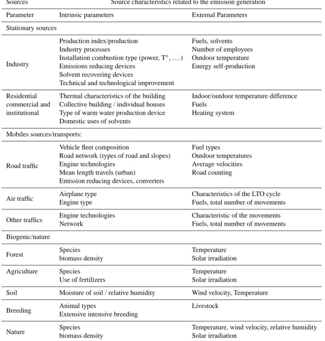
Table 1. Principal parameters involved in the emission scenario calculations.
Sources Source characteristics related to the emission generation
Parameter Intrinsic parameters External Parameters
Stationary sources
Industry
Production index/production Fuels, solvents
Industry processes Number of employees
Installation combustion type (power, T◦, . . . ) Outdoor temperature Emissions reducing devices Energy self-production Solvent recovering devices
Technical and technological improvement
Residential Thermal characteristics of the building Indoor/outdoor temperature difference commercial and Collective building / individual houses Fuels
institutional Type of warm water production device Heating system Domestic uses of solvents
Mobiles sources/transports:
Road traffic
Vehicle fleet composition Fuel types
Road network (types of road and slopes) Outdoor temperatures
Engine technologies Average velocities
Mean length travels (urban) Road counting Emission reducing devices, converters
Air traffic Airplane type Characteristics of the LTO cycle
Engine type Fuels, total number of movements
Other traffics Engine technologies Characteristic of the movements
Network Fuels, total number of movements
Biogenic/nature
Forest Species Temperature
biomass density Solar irradiation
Agriculture Species Temperature
Use of fertilizers Solar irradiation
Soil Moisture of soil / relative humidity Wind velocity, Temperature
Breeding Animal types Livestock
Extensive intensive breeding
Nature Species Temperature, wind velocity, relative humidity
biomass density Solar irradiation
factor which links the activity of the source and the emis-sion of p during 1t. In this equation, one can modify the emissions by changing the activity of the sources, the char-acteristics, the location or the emission factors of the sources. However, Eq. (1) can be more complex and can involve sev-eral parameters included in the activity or in the emission factor, which leads to various scenarios. The parameters can be grouped into two categories:
– Intrinsic parameters. They are specific to the
character-istics of the sources and the emission generation pro-cesses. These parameters are usually related with the emission factors.
– External parameters. They can change the emission
lev-els, independently of the source characteristics. These parameters are usually included in the activity factors. Table 1 gives a summary of the parameters used in emis-sion inventories which can be modified to generate different emission scenarios. One comment can be necessary to pre-cise one point concerning the transport source category: the counting (number of vehicle per unit time) for the road traffic and the number of movements for the other traffics are gener-ally considered as external parameters. Nevertheless, it can also be assumed as intrinsic ones when the counting or the number of movements for each detailed categories of mobile
Fig. 1. General method of impact assessment using emission reference and scenarios.
sources are used to elaborate emission factors of the whole fleet of mobile sources. One can notice that for several source categories, the emissions depend on meteorological param-eters such as temperature, solar radiation or wind velocity. This means that the meteorological conditions can modify the emitted fluxes of these sources. Some of them are con-trolled by meteorological parameters, such as biogenic and natural sources. These latter parameters are not considered when creating scenarios, but generally they are used to per-form sensitivity analyses of the emissions. Modifying them allows one to quantify the variability of these emissions re-lated to the environmental conditions. Thus, the dependence of the emissions on these parameters can be evaluated and the accuracy of the parameters can be defined to avoid large emission uncertainties. For instance, since the emissions of a large surface source such as a forest depend on the temper-ature, their calculation requires the knowledge of the tem-perature over the whole area concerned. As the sensitivity of this parameter (depending on the tree species constituting the forest) is important, the description of the temperature field over the area must be accurate to minimize the uncertainties on the emissions.
2.3 The main types of air quality management emission scenarios
According to the goals of the emission abatement strategy and further use of the emission scenarios, different ways of creating emission scenarios are possible. The main types can be derived from existing emissions on different time frames: yearly down to hourly. Since our main research interest deals with air quality management at the mesoscale, we will focus on middle and short term strategies. In that respect, the sce-narios are based on the following changes of the parameters previously described:
– modification of emission factors (EFp,S,1t) related to
changes of the source characteristics such as the
com-position of the fuels, technology improvements (pro-cesses, engines, reduction emission devices, etc.), en-ergy savings, the use of solvent recovery devices for anthropogenic sources, and vegetation species in forest and agriculture for biogenic sources,
– modification of the sources’ activities (Ap,1t) such as
the production, traffic volume changes, and biomass factors changes,
– changes of the intrinsic source characteristics:
pro-cesses, fuels, mobile source fleet, vegetation species,
– localization of the emission sources: break down of
activities, new source locations, land use changes (ur-ban, agriculture, forest area, water surface modifica-tions). Note that the land use changes may also have climatological impacts which can induce feedback on emissions through albedo, ground temperature, heat changes,
– modification of the time distributions of the emission
with all intrinsic parameters unchanged.
The other aspects of the creation of emission scenarios concern the purpose of the air quality management and/or the abatement strategies. First, the emission scenarios can focus on one or more particular source categories to assess the impact of emission changes for these sources. This type of scenario is very useful to quantify the impact of regula-tions on specific emission sources. Second, the construction of the scenarios can be based on regulation goals to be ap-plied in terms of concentration or emission levels. In case of emission abatement, the sources have to be modified (activ-ities, emission factors) to reach theses levels. The goal is to quantify the improvements generated by this regulation. An-other use of this method of creation is to orient a scenario to concentration or exposure levels to be reached. This can be
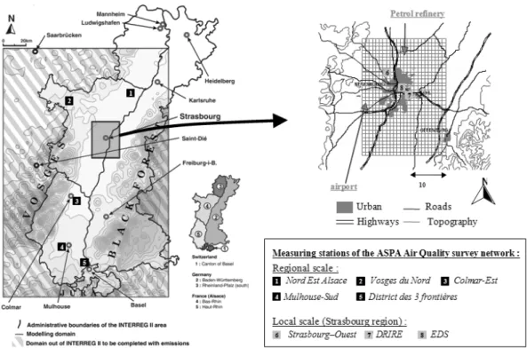
Fig. 2. Geographical location of the regional and local investigation domains.
very complex since different approaches can be used to mod-ify emission levels, the chemical composition of emissions (to decrease specific secondary pollutants) or the emission time distributions according to meteorological conditions (to favor efficient dispersion of pollutants). In this case, several scenarios have to be tested to obtain the most efficient way to reach the objectives, especially if cost effectiveness is a concern.
3 Scenarios and air quality modeling
In this section, we present two examples of applications of emission scenarios. The emission scenarios consider the change of one specific emission category and their impact on air quality at local and regional scales. Both reference case emissions and scenarios are then used as input data to the chemical mechanism of the air quality model. The last step is the comparison of the respective simulated pol-lutant concentration fields to assess the impacts of emission changes (Fig. 1). The first example concerns the impact of the installation of an urban tramway instead of the road traf-fic in the old centre of Strasbourg (Gallardo, 2000), and the second deals with the impacts of using modified car fuels (oxygenated and reformulated fuels) at local (Strasbourg ur-ban area) and regional (upper Rhine valley) scales (Vinuesa, 2000; Vinuesa et al., 2003). All the simulations use the model EUMAC Zooming Model – EZM (Moussiopoulos, 1995) composed of two independent models: a meteorologi-cal mesosmeteorologi-cale model MEMO and a reacting transport model
MARS. Different chemical mechanisms have been used to fit with the goal of each study.
3.1 Areas and period of interest
The regional domain of investigation is the whole up-per Rhine valley (Fig. 2). This area of 144 km (East– West)×216 km (North–South) regroups parts of three coun-tries: Switzerland, Germany and France. It is a densely pop-ulated (about 6.3 million inhab. and 300 inhab. km−2) and industrialized region. The Alsace region is located in the western part of the upper Rhine valley and regroups 1.71 M. inhabitants on about 8250 km2. Two main highways cross north to south this valley and draw heavy local and trans-border road traffic. The upper Rhine valley is surrounded by three mountainous chains: the Vosges (west), the Black forest (south east) and the Jura (east south). The modeling domain has been chosen to preserve the geographical and dy-namic unity of the valley. The topography allows the emer-gence of frequent temperature inversion especially under an-ticyclonic weather conditions. For several years, emission abatement strategies appeared necessary given the increase of photochemical pollution episodes. Also, this region is very sensitive to air pollution due to these meteorological and climatological conditions (Adrian and Fiedler, 1991; Schnei-der et al., 1997). Further information can be found in REK-LIP (1995, 1999), and Ponche et al. (2000).
The local domain is included in the regional one and consists of the German-French urban area of Strasbourg– Offenburg. It has been selected to allow the study of emission
Table 2. Summary of the emission inventory used for the extended urban area of Strasbourg, extracted from the hourly REKLIP emission inventory for the 16 September 1992.
Emission Sources Emissions for the 16.09.1992 in t/day
SO2 NOx VOC CO
Road and air Traffic1(Exhausts and evaporation) 2.29 33.89 24.86 112.61 Points source emissions (combustion and processes) 24.34 5.55 6.98 1.14 Area sources emissions (including other industries, residential and service sectors) 8.38 2.82 3.60 2.68
Total 35.01 42.26 35.44 116.43
1Airport contribution represents between 1–4% of the total traffic emissions for the different compounds.
Fig. 3. Impact of the road traffic change in the Centre of Strasbourg (Scenario) compared with the reference case simulation (Computed) and concentration measurements (Measured) of O3(upper left), CO (upper right), NO2(lower left) and NO (lower right) at two stations (DRIRE
and EDS) of the ASPA air quality measuring network. These two stations are located in the Centre of Strasbourg (see Fig. 2).
impacts over a typical urban area. This domain is located across the Rhine river and includes the urban community of Strasbourg (420 000 inhab.), the communities and cities (Offenburg and Kehl) of the administrative district Ortenau (90 000 inhab.) and the other communities around the admin-istrative limits to complete the square domain (44 000 inhab. for the French part and 16 000 for the German part). The area covers 24 km (East–West)×32 km (North–South) and the to-tal number of inhabitants was about 590 000 in 1995.
The results of the impact studies presented in the following are summarized from previous works dealing with the pho-tochemical pollution episodes of 15–16 September 1996 and of 9–15 May 1998. During these periods, the anticyclonic
conditions were favoring photochemical pollution, i.e. north-eastern low wind flows all over the region with temperature about 3 to 5◦C above the seasonal average. The low wind ve-locities and strong temperature inversion prevented the dis-persion of the emitted pollutants (especially issued from ur-ban area and heavy traffic sources). For example, during the May 1998 episode, these summer-like conditions led to 28 overflows of the information threshold of the ozone directive of the European Union (180 µg m−3×1 h of ozone exposi-tion) in the urban area of Strasbourg.
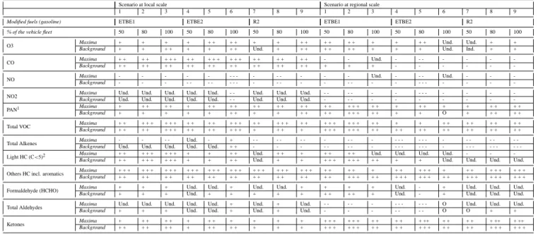
Table 3. Brief overview of the results obtained for the main chemical species at local (urban area of Strasbourg) and regional (upper Rhine valley) scales.
Scenario at local scale Scenario at regional scale
1 2 3 4 5 6 7 8 9 1 2 3 4 5 6 7 8 9
Modified fuels (gasoline) ETBE1 ETBE2 R2 ETBE1 ETBE2 R2
% of the vehicle fleet 50 80 100 50 80 100 50 80 100 50 80 100 50 80 100 50 80 100 O3 MaximaBackground ++ ++ ++ + ++ + ++ + ++ + Und.+ ++ + ++ + + ++ + + ++ + ++ ++ ++ + Und.Und. Ind.Und. ++ ++
CO MaximaBackground + ++ + + ++ + + + ++ + + ++ + + + ++ + + ++ + + + ++ + + ++ + + ++ + -+ +- +Und. -- -- - -- -- -- -
-NO MaximaBackground -- -- -- - -- -- - - - -- - - -- - -- - -- -- - -- -Und. -- - - -- - -Und. -- -- -
-NO2 MaximaBackground Und.Und. Und.Und. Und.Und. Und.Und. Und.Und. - -- - Und.Und. Und.Und. Und.Und. - -- - -- - -- -- -- - - -- -- -- - -PAN1 Maxima + + + + + + + + + + + + + + + + + + + + + + + + + + + + + + + +
Background + + + + + + + + + + + + + + + + + + + + O + + + + +
Total VOC MaximaBackground + ++ + + + ++ + + + ++ + + + ++ + + ++ + + + ++ + + ++ + + ++ + + + ++ + + ++ + + + + ++ + + + ++ + + ++ + ++ + ++ + + ++ + + ++ + + ++ +
Total Alkenes MaximaBackground -Und. -Und. - -Und. Und.Und. -Und. + ++ -- - -- - - -- -- - - -- - -- - - -- - - - - -- - - -- - - -- - - - -- - - - -Light HC (C<5)2 Maxima + + + + + + + + + + + + Und. + + + + + + + Und. Und. Und. Und. - -
-Background + + + + + + + + + + + + Und. + + + + + + + + + + + + Und. Und. Und. Und. Others HC incl. aromatics MaximaBackground + + ++ + + + ++ + + + ++ + + ++ + + + + ++ + + ++ + + + ++ + + + ++ + + + + ++ + + ++ + + + ++ + + ++ + + ++ + + + ++ + + + ++ + + ++ + + + ++ + + + + ++ + +
Formaldehyde (HCHO) MaximaBackground ++ ++ ++ Und.Und. Und.+ ++ +Und. +Und. ++ ++ + + ++ ++ Und.Und. -- ++ Und.Und. Und.Und. Und.Und.
Total Aldehydes MaximaBackground Und.+ Und.+ Und.+ Und.Und. Und.Und. ++ Und.Und. ++ Und.Und. - -- -- - -- - -- - - - -- - - OO OUnd. +Und. Und.+
Ketones Maxima + + + + + + + + + + + + + + + + + + + + + + + ++ + + + + + ++ + ++ Background + + + + + + + + + + + + + + + + + + + + + + + + + + + + + + + + + + + + +
1PAN: peroxy-acetyl-nitrate
2HC: hydrocarbons (number of carbon C<5)
Und.: Undefined impact, the spatial distribution does not allow aclear trend on the whole domain. O: no significant impact on the whole domain
+, + +, + + +: more and more positive impact s (reductions of simulated concentrations) -, - -, - - -: more and more negative impacts (increases of simulated concentrations).
3.2 Impact of local road traffic changes
In view of the building of the tramway through the old part of the city, which included the removal of all road traffic in this old centre of Strasbourg (6 km2of dense small streets), some scenarios have been elaborated to assess the future impact of this road traffic change. A high resolution emission inven-tory (1×1 km2×1 h) was established for 16 September 1992 corresponding to an ozone pollution episode (see Table 2). This inventory was created from the REKLIP hourly emis-sion inventories (Ponche et al., 1995, 2000). The road traffic from the old city centre has been displaced around the centre with the help of a rough traffic model to preserve the consis-tency of the road traffic volume. Thus, the total hourly emis-sions have not been significantly decreased; only the spatial distribution has been changed. The simulations have been performed with EZM and with the chemical mechanism KO-REM (Flassak et al., 1993). The results at two representa-tive locations of the centre of Strasbourg are summarized in Fig. 3. The simulated impact of this change is very limited and concerns only the domain where the emission reductions (road traffic) have been applied (curves “Scenario” in Fig. 3). It has led to a small increase of the ozone peak and a decrease
of NOxand CO concentrations levels. A complete
descrip-tion of this study can be found in Gallardo (2000).
3.3 Impact of local and regional emission changes due to modified car fuels
Another example to illustrate the impact study of differ-ent emission scenarios is the study performed within the framework of the French program AGRICE (Agriculture for Chemistry and Environment). This study aims at quantify-ing the possible impacts of usquantify-ing three modified car fuels: a gasoline car fuel named ETBE1 containing 15 weight % of Ethyl tertio-butyl Ether (ETBE), a reformulated gasoline (R2), and one both reformulated and containing ETBE (so called ETBE2). The use of alternative fuels has been sug-gested at the end of the eighties in order to improve urban air quality by reducing combustion-related pollution. Indeed, reformulating the fuel (modification of the chemical compo-sition of the fuel, e.g., by lowering of the aromatic fraction, and/or addition of oxygenated compounds, as here the ethyl-tertio-butyl-ether or ETBE) allows the modification of the composition of the emissions due to the road traffic. Only a brief overview is given below and all further details can be found in Vinuesa (2000) and in Vinuesa et al. (2003). The
Fig. 4. Example of quantified impacts on daily average concentrations of O3, NO2and VOC obtained for the car fuel added with 15 weight %
of ETBE (without reformulation) used by 50% and 80% of the gasoline passenger car fleet at local and regional scales, respectively. Positive negative values, respectively, corresponds to decrease – increase of concentrations compared to the simulation with the reference emission inventory.
scenarios have been created from the PRIMEQUAL and IN-TERREG II emission inventories at local scale, i.e. the Stras-bourg area, and regional scale, i.e. the upper Rhine valley, re-spectively. The existing emission inventories have been con-sidered a reference. Then, the road traffic contribution from the gasoline passenger cars has been extracted and modified to take into account different fleet car fractions using these modified fuels (30, 50, 80 and 100% at local scale).
Table 3 gives an overview of the results obtained at lo-cal and regional slo-cales. These results show that the major positive impacts (reduction of resulting concentrations) on air quality at the local scale were obtained when more than 50% of the vehicle fleet is using modified car fuels. In the urban area the road traffic contribution is much more im-portant compared to the regional scale. Thus, the impacts obtained at local and regional scales vary somewhat due to the differences in spatial distribution emissions. At local scale, the VOC (up to 20–25% for background concentra-tions, and 45% for the peak concentrations) especially the aromatic fraction, the CO (8–12% and 25%, respectively), are reduced. Lower concentration reductions are simulated for the ozone (1–3 and 3–6 %, respectively) the ketones, and the peroxy-acethyl-nitrate (PAN). On the contrary, global
negative impact trends (increase in concentrations) have been obtained for NOxand the alkenes, even if very locally, some
positive impacts are simulated. For aldehydes, there is no clear trend. At regional scales, positive impacts are obtained for the VOC, PAN and ketones similar to what is obtained at local scale and the reduction of ozone levels is still small. However for NOx, alkenes, CO and the total aldehyde group,
significant negative trends are found. This study has allowed quantifying the possible effects of these modified fuels used by different fractions of the gasoline passenger car fleet as illustrated in Fig. 4.
4 The 2015 European emission regulations applied to the upper Rhine valley
In France, since the Law on air and the rational use of en-ergy has been established in 1995, each region and major city (over 200 000 inhabitants) have to define a Regional Plan for Air Quality (PRQA) and Atmospheric Protection Plan (PPA), respectively. These regulations are generally intensifying the existing European guidelines on air quality, to reach the ob-jectives defined for the whole EEC. Within the framework of the PRQA of the Alsace region, the Regional Direction of
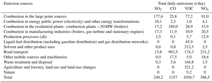
Table 4. Total daily emissions in tons per day for the 11 May 1998 for the whole INTERREG II domain.
Emission sources Total daily emissions (t/day)
SO2 CO VOC NOx
Combustion in the large point sources 177,6 25,8 77,2 91,0
Combustion in energy public power (electricity) and other energy transformations 10,1 2,5 1,0 4,1 Combustion in the residential plants: combustion plants <50 MW (boilers) 17,2 189,0 28,9 15,9 Combustion in manufacturing industries (boilers, gas turbine and stationary engines) 17,3 11,9 10,9 20,5
Production processes (all) 2,5 0,1 5,7 12,9
Liquid fuel distribution (including gasoline distribution) and gas distribution networks) 0 0 45,9 0
Solvent and other product uses 0,6 0,8 212,5 2,5
Road transport 13,8 903,5 174,3 231,2
Other mobile sources and machineries 0,9 17,5 5,0 18,6
Waste treatment and disposal 0,3 5,6 164,8 1,5
Agriculture and forestry, land use and land-use changes 0 0 321,2 0
Nature 0 0 9,2 0
Total 240,2 1157 1056,7 386,5
Research, Industry and Environment (DRIRE) of Alsace has charged our Laboratory to perform impact studies of abate-ment strategies on the upper Rhine valley. The present study has two main objectives: (1) to determine the changes in ozone and NOxlevels if the future European regulations
(re-ferring to the year 2015) would have been applied for the whole area during the photochemical episode of the 9–15 May 1998 and (2) to provide a practical example, that can be included in a PRQA, of the benefits of using air qual-ity modeling coupled with emission scenarios for air qualqual-ity management. For this purpose, emission reduction scenarios have been elaborated jointly with the “Prefecture” (which are the executive state authorities), the DRIRE (charged to check the application of the formal directives), the Centre d’Etude Technique de l’Equipement (CETE) de l’Est (charged with all questions regarding the road transport including the road management network out of the cities) and the Association de Surveillance et d’´etudes de la Pollution Atmosph´erique (ASPA) of the Alsace region which is in charge of the survey and measuring air quality network. The modified emission inventories are used as input data in simulations performed with the EZM air quality model and the results are compared with the base case modeling using the existing emission in-ventory.
4.1 The PRQA emission scenarios
The emission scenarios are based on the hourly emission in-ventories created for the period of 9–15 May 1998 (Table 4) and for the air quality modeling of this ozone episode (Pal-lar`es et al., 1999a, b). These hourly emission inventories are derived from the yearly INTERREG II emission inventories (INTERREG II, 2000; Pallar`es et al., 1999c). The INTER-REG II emission database is a 1 km×1 km emission inven-tory for the whole upper Rhine valley for the reference year
1997 and includes both anthropogenic and biogenic sources. Both time distribution functions and hourly data are used to reach the hourly resolution. As far as hourly data are avail-able, they allow us to calculate specific hourly emissions. In case of missing data, representative time function distribu-tions are created according to complementary data on the ac-tivities and behaviors of the emission sources. The emission and activity sources are classified using the European nomen-clature SNAP 97 (Selected Nomennomen-clature for Air Pollution actualized in 1997). Special attention is devoted to orient this emission database structure to spare actualization proce-dures including emission scenario generation. Two emission scenarios, both referring to the year 2015, are used. The first scenario (SC1) describes the evolution of the emissions when only the incoming European emission evolution and regula-tions are taken into account. The second (SC2) is based on the same evolution, but with additional constraint of local and regional regulations about pollutant emissions. The re-sults obtained for these new emissions inventories are sum-marized in Table 5.
In SC1, the emissions due to the fixed installation of com-bustions are issued from three sectors: industry, residential (individual housing) and service sectors. The sulphur con-tent of heating oil (0.2 wt% for the base case) has been low-ered to 0.1 wt% in all combustion processes involved in these latter sectors. Incoming improvements in heating technology are supposed to reduce the NOx emissions by 2% and the
CO emissions between 3 and 8% for some activity sectors. For chemical industrial processes, the NOxemissions are
re-duced by 5% except for cement and paper factories where the reductions reach 30% and 50%. For the point sources, the use of natural gas increases and the other fuels are re-duced by 8% in TOE (Tons Oil Equivalent). For the waste treatment sector, emissions of VOCs are reduced by a factor of 2 except for domestic waste incinerators where emission
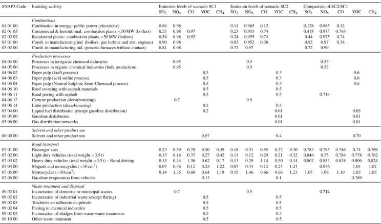
Table 5. Weighting factors per code SNAP3 level description 3) concerned by the application of the regulations for the SC1, SC2 and relative differences (in %) of SC2 compared to SC1. The emission level references are those of 1998 which correspond to 1.00. This table contains only the emitted compounds which are subject to reductions. The emission levels of the other compounds are unchanged compared to 1998.
SNAP3 Code Emitting activity Emission levels of scenario SC1 Emission levels of scenario SC2 Comparison of SC2/SC1
SO2 NOx CO VOC CH4 SO2 NOx CO VOC CH4 SO2 NOx CO VOC CH4
Combustions
01 01 00 Combustion in energy: public power (electricity) 0.86 0.98 0.11 0.965 0.12 0.128 0.985 0.12
02 01 03 Commercial & Institutional: combustion plants <50 MW (boilers) 0.55 0.98 0.97 0.23 0.955 0.74 0.418 0.975 0.763
02 02 02 Residential plants: combustion plants <50 MW (boilers) 0.54 0.98 0.92 0.24 0.955 0.74 0.44 0.975 0.74
03 01 00 Comb. in manufacturing ind. (boilers. gas turbine and stat. engines) 0.90 0.98 0.83 0.952 0.38 0.92 0.97 0.38
03 02 00 Comb. in manufacturing ind. (process furnaces without contact) 0.81 0.98 0.72 0.97 0.72 0.99
Production processes
04 04 00 Processes in inorganic chemical industries 0.95 0.5 0.53
04 05 00 Processes in organic chemical industries (bulk production) 0.95 0.5 0.53
04 06 02 Paper pulp (kraft process) 0.5 0.3 0.6
04 06 03 Paper pulp (acid sulfite process) 0.5 0.3 0.6
04 06 04 Paper pulp (Neutral Sulphite Semi-Chemical process) 0.5 0.3 0.6
04 06 10 Roof covering with asphalt materials 0.5 0.5
04 06 11 Road paving with asphalt 0.5 0.5 0.714
04 06 12 Cement production (decarbonizing) 0.7 0.5
04 06 14 Lime production (decarbonizing) 0.5 0.5
05 04 00 Liquid fuel distribution (except gasoline distribution) 0.2 0.01 0.05
05 05 00 Gasoline distribution 0.01 0.01
05 06 00 Gas distribution networks 0.01 0.01
Solvent and other product use
06 00 00 Solvent and other product use 0.57 0.4 0.70
Road transport
07 01 00 Passenger cars 0.23 0.39 0.70 0.50 0.39 0.18 0.31 0.55 0.37 0.30 0.783 0.795 0.786 0.74 0.769
07 02 00 Light duty vehicles (total weight <3.5 t) 0.13 0.16 0.37 0.27 0.42 0.11 0.12 0.29 0.21 0.32 0.846 0.75 0.784 0.778 0.762
07 03 02 Heavy duty vehicles (total weight >3.5 t) – Rural driving 0.15 0.34 1.36 0.62 0.17 0.13 0.29 1.14 0.50 0.14 0.867 0.853 0.838 0.806 0.824
07 04 00 Mopeds and motorcycles (<50 cm3) 0.07 0.46 0.12 0.23 1.22 0.07 0.44 0.12 0.24 1.24 0.956 1.04 1.02
07 05 00 Motorcycles (>50 cm3) 0.14 1.35 0.60 0.64 1.19 0.15 1.46 0.66 0.66 1.23 1.07 1.08 1.10 1.03 1.03
07 06 00 Gasoline evaporation from vehicles 0.13 0.1 0.769
Waste treatment and disposal
09 02 01 Incineration of domestic or municipal wastes 0.7 0.5 0.714
09 02 02 Incineration of industrial waste (except flaring) 0.5 0.5
09 02 03 Torch`eres en raffinerie du p´etrole 0.5 0.5
09 02 04 Flaring in chemical industries 0.5 0.5
09 02 05 Incineration of sludges from waste water treatments 0.5 0.5
09 10 00 Other waste treatment 0.5 0.5
reductions reach 30%. For the mobile sources, especially road traffic, the incoming motor technology, the reformula-tion and the decrease of the weight sulphur content of car fuels are considered by the CETE to balance the increase of the volume road traffic. The same hypothesis has been made for air, railway and fluvial traffic. Biogenic emissions are supposed to remain the same.
The SC2 scenario is based on the same European regu-lations as SC1 but includes more restricting reguregu-lations that correspond to a regional political will to reduce emissions. For all the fixed installations of combustion, all charcoal fuel types are replaced by heating oil with all fuel oils contain-ing 0.05 wt% of sulphur. Incomcontain-ing improvements in heatcontain-ing technology reach those of the point sources leading to a re-duction of NOx emission levels of 5% (compared to 2% in
SC1). For the other activity sectors involving combustion, emission reductions for SO2go from 14% to 89%, and 26%
to 88% for CO. The emissions due to the industrial processes for some specific activities are reduced to 50% for NOxand
in a range between 50% and 99% for the VOCs. For instance, the NOxemissions are reduced by 50% in chemical
indus-trial processes except for paper factories where the reduction reaches 70%, and the VOC emissions from domestic waste
incinerators are reduced by 50% (compared to 30% in SC1). For transports, the development of public transportation at local and regional scales (extension of bus and tramway net-works, increase of urban pedestrian area) and additional con-straints on personal cars at national level (increase of car fuel taxes, balancing of the diesel and gasoline prices) allow to reduce emissions from road traffic between 17% and 19% for CO, NOxand VOC compared to the SC1. For the other
traffic, this scenario considers a decrease of the diesel rail-way traffic and of fuel consumption (about 10%) leading to lower the emissions by more than 50% (56% for SO2, 57%
for NOx54% for the VOCs and 60% for CO). The air traffic
emissions are reduced by 2% per year.
4.2 Impacts of the scenarios SC1 and SC2 on regional air quality
4.2.1 Model specifications
The simulations are performed using EZM and the numeri-cal setup of the simulation is briefly summarized here. The modeling domain represents an area of 144 km×216 km with a prescribed grid of 36×54 points in the horizontal leading to a of 4 km×4 km. In the vertical direction, 35 points are
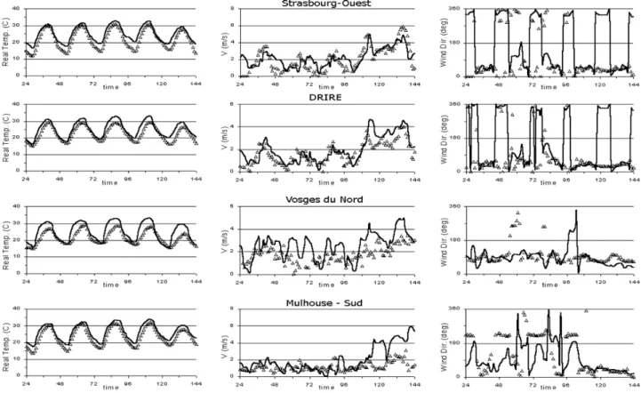
Fig. 5. Evolution of the temperature (first panel from left to right), horizontal wind intensity velocity (second panel) and direction (third panel) for a selection of the Alsacian measuring sites of the ASPA Air Quality survey network. The solid lines indicate the model results. The period represented is the 10 to 14 May 1998. “DRIRE” measuring station is located in the centre of the urban area of Strasbourg, “Strasbourg-Ouest” and “Mulhouse-Sud” are suburban measuring sites and “Vosges du Nord” is a rural one in a forested area (located 60 km North East of Strasbourg). All these locations are mentioned in Fig. 2.
used to represent 6 km. The calculations are performed for the period of 9–14 May 1998. The initialization and bound-ary conditions are determined using vertical soundings pro-vided by the ASPA for the first 1200 m and by the Deutsche Wetterdienst (DWD-Stuttgart, 100 km north-east from Stras-bourg) for the altitudes above this height. The boundary con-ditions and the background concentrations of reactants are extracted from the regional network measurements done by the ASPA-Strasbourg. Therefore, the measurements from rural stations are used to evaluate the background ozone levels (around 70 ppb). A measurement station located in the core of the valley between Strasbourg and Karlsruhe, the so-called North-East Alsace, allows to take into account the urban plume coming form Karlsruhe region (with NOx
levels around 9 ppb). Using these measurements, the ratio NMVOC/NOxis estimated at 2.5. Keeping constant, in time
and in space, the boundary conditions allow obtaining a clear analysis of the effect of the emission scenarios. In order to reduce the CPU demand, the chemical mechanism KOREM (Flassak et al., 1993) is used. This latter rather simple mech-anism has shown its ability to account for ozone formation and depletion in the atmospheric boundary layer.
4.2.2 Benchmark simulation result
In Fig. 5, the time evolutions of the temperature (first panel from left to right), horizontal wind velocity (second panel) and direction (third panel) for a selection of the Alsacian me-teorological sites are presented. The differences obtained in the temperature are mainly due the effect of averaging pro-cedures on the topography and the land-use over 4×4 km2. Nevertheless, the comparison between the measurements and the model results show a good agreement. One can notice that even the change of wind regime, i.e. from low to high geostrophic wind at the end of the week for the north part of the modeling domain, is reproduced with good accuracy. The time evolution of the ozone concentration for a selection of the Alsacian meteorological sites are presented in Fig. 6. Here also, the model results and the measurements are in a good agreement; the diurnal cycle is well reproduced even if the stations are close to or in urban areas and the horizontal resolution is 4×4 km2.
Since the pollution situation was not dramatically chang-ing from day to day, only the results obtained for a schang-ingle day of simulation, e.g. 12 May are described (see Fig. 7). During
Fig. 6. Evolution of the ozone concentrations for a selection of the Alsacian pollutant measurement sites. The solid lines indicate the model results. The period represented is the 10 to 14 May 1998. “Nord-Est Alsace” and “Vosges du Nord” stations correspond to rural and mountainous sites located 60 km north east of Strasbourg and 90 km north of Strasbourg, respectively. “Strasbourg-Ouest”, “Colmar-Est”, and “Mulhouse-Sud” correspond to semi-urban measuring stations. The measuring station “District des 3 fronti`eres” is also an semi urban one, located close to the Swiss-German- French border, south east of the domain. All theses sites are also indicated on the maps of Fig. 2.
the morning and the late afternoon, the wind flow is mainly driven by usual breeze phenomena that can be encountered in shallow valleys. Since the geostrophic wind shows low lev-els, the impacts of valley and mountain breezes are enhanced. Under such a low shear condition, the chemical transforma-tions of the pollutants take place in a convective boundary layer driven mainly by turbulence during the day. As a re-sult, the flow pattern over urban areas, such as Strasbourg or Mulhouse for instance, shows a strong turbulent structure. Nevertheless, since the shear is low, the pollutants are mainly not advected and the urban plume remains over the core of the valley.
In the early morning, ozone levels are driven by ozone de-pletion process due to NO. Therefore, the lowest ozone lev-els are found close to high NO emission sources such as ur-ban areas or heavy traffic road. Over the mountainous areas, ozone levels are still high since they are related to the
accu-mulation of the ozone produced the day before (no chemical sink in these regions). In the mid-morning, the breezes col-lapse and start to invert. As a result, the ozone produced in urban plumes transported by valley breezes enhances the ozone levels over the mountains. From this period until the late-afternoon, the production process of ozone in the whole valley becomes predominant. The combined contributions of the main city plumes allow the formation of high lev-els of ozone (more than 100 ppb or 200 µg/m3) in almost the whole domain. At sunset, since the photolytic source of ozone collapses, the ozone levels over the cities or the core of the valley decrease dramatically. Over the rural regions, and particularly the mountains, ozone accumulates leading to the formation of ozone tanks reservoirs which remain during the night.
Fig. 7. Ozone concentration fields for 12 May 1998.
4.2.3 Effects of the emission scenarios
The results on the spatial distribution of the impacts show global improvement trends for the air quality over the whole region due to lower emissions. On the right hand side of Fig. 8, the percent change of the NOx concentration field
for SC1 is presented. One can notice that this first scenario allows an important decrease of NOxlevels over the whole
domain which can reach even more than 90%. For ozone, the reductions can reach more than 10 ppb over areas where ozone levels show their maximum (see l.h.s. of Fig. 8). Nev-ertheless, one can notice some increases of ozone levels in the urban areas, in spite of the reduction of primary pollu-tants. The tropospheric ozone levels are issued from a net balance between formation and destruction processes, and the chemical compounds which generate ozone are also tak-ing part in its depletion. Formation and/or destruction de-pends in fact upon physical and chemical atmospheric con-ditions such as temperature, solar radiation, relative concen-trations of NOx, VOCs and especially NOx/VOC ratios. In
urban areas, during photochemical episodes, the emission of NOx and VOC leads to lower ozone levels with high daily
variations compared to rural areas (including mountainous areas), where higher and more constant levels can be ob-served. The destruction of ozone is more efficient in urban
Fig. 8. Effects of SC1 on the concentration fields of ozone and NOx
for 12 May 1998 at 13:00 LST. The left figure represents the differ-ence between the scenario and the referdiffer-ence case for ozone. On the right figure, the percentage of increase of the NOxconcentration
field is given. Notice that in both cases a positive/negative value accounts for an increase/decrease of concentration. The topography is represented with solid lines.
areas due to higher emissions. Then, part of the urban ozone can be transported over rural areas where its destruction is low (due to lower emission levels). These processes lead to ozone accumulation over this type of area. The effects of the reduction emission scenarios are to modify the ozone balance by decreasing the ozone destruction rather than the genera-tion over the urban areas and by lowering the ozone produc-tion and accumulaproduc-tion over the rural areas. Similar results are obtained for SC2.
For SC1, the impacts on the NOxconcentrations are much
more significant than those for ozone. A general decrease of up to 90% of NOxconcentrations is observed. This means
that the emission abatement strategy seems very efficient. SC2 allows a higher decrease up to 30% compared to SC1 on the main part of the domain. However a small increase of NOxis calculated for SC2 over the area of Karlsruhe (10–
15% as compared to SC1). This can be explained by the fact that the SC2 concerns only the Alsace region. As mentioned previously, the major effect of the large decrease of the NOx
concentrations is the decrease of ozone in rural and moun-tainous areas and the increase of the ozone concentrations in the highly urbanized area.
An alternative to evaluate the impact of emission scenar-ios on air quality is to define parameters that can be used to evaluate the concept of threshold and accumulated levels of pollutants. Studies of the impacts of ozone on agricul-tural crops and forests have resulted in the establishment of critical levels using long-term exposure measures. One of these measures is the accumulated excess ozone (Fuhrer and Achermann, 1991). This index is referred to as AOTX that represents the accumulated excess of ozone over a threshold of X ppb. In fact several AOT can be defined. In this pa-per, we focus on the AOT40, AOT55 and AOT60. These
Fig. 9. Effects of the SC1 on the AOT40, 55 and 60.
AOT represent the total cumulative amount of ozone lev-els higher then 40 ppb as an hourly average during daytime, higher than 55 ppb as an hourly average between 13 and 20 LST and higher than 60 ppb as daily maxima, respectively. These parameters are calculated for the whole period of the experiment. Figure 9 shows the effect of SC1 on such pa-rameters. Some general conclusions can be drawn from this figure. The background levels of ozone, as represented by the AOT40, are reduced by approximately 10% in the main part of the valley. The highest daily value of ozone (AOT55) and the daily maximum of ozone (AOT60) are reduced by 10 to 40% everywhere apart from the urban areas where the in-crease of the AOT55 and the AOT60 can reach 70%. These results show a global trend of improved air quality standards by applying the emission scenarios. Nevertheless, as men-tioned previously, the ozone levels and, thus the AOTs, are increasing in urban areas. Since the emission scenarios are based on the reduction of the emission of ozone precursors such as NOx, and since, in these areas, the ozone is driven by
depletion processes such as oxidation by NO, the ozone de-pletion is less efficient. On the other hand, the generation of ozone in urban plumes is lower and the AOTs are decreasing in the rural areas that constitute the main parts of the valley.
A first step to estimating the population exposure to ozone pollution is to determine the surface of the domain concerned by high levels of ozone. We determine the surface where
Table 6. Total daily surface concerned by the excedance of the European information threshold for ozone. The surfaces are given in km2.h.
Benchmark Scenario SC1 Scenario SC2
Sun. May 10 16 572 12 914 12 989 Mon. May 11 25 605 16 274 15 154 Tue. May 12 41 356 8510 7614 Wed. May 13 26 351 15 527 15 229 Thu. May 14 9854 4330 4255 Average 23 947.6 11 511.0 11 048.2
ozone levels are exceeding the hourly information thresh-old of ozone (e.g. 180 µg m−3×1 h of ozone exposition). As a result, we access a population exposure index that is ex-pressed in square kilometers – hour units. In Table 6, we present the total daily surface (area of the domain×24 h) where ozone levels are exceeding the information threshold for the ozone calculated for the reference case (where no emission scenario is used) and for the scenario SC1 and SC2. One can notice that the hourly-areas affected by the overflow of this threshold are reduced by applying emission regula-tion scenarios. In fact, for the whole polluregula-tion episode, these areas are reduced by more than 50%. The next step of this study could be to correlate these numbers with the amount of people living in such areas and the sub-grid topography. Then it will be possible to estimate the population exposure to pollution.
5 Summary and conclusion
We have illustrated the possible use of emission scenario for air quality management purpose by presenting the effect of three emission abatement strategies: the impact of the instal-lation of the urban tramway in the old centre of Strasbourg, the use of oxygenated and reformulated car fuels at local and regional scales, and the application of the future European regulations. In this latter application, which is the most re-fined, the results show global improvement trends for the air quality over the whole region due to lower emissions (be-tween 10 and 90% of general decrease for NOxand between
5 and 25% of decrease in rural and mountainous areas for ozone). Nevertheless, there are some increases in ozone lev-els (up to 30%) in the urban areas in spite of the reduction of primary pollutants. This can be explained by consider-ing that the tropospheric ozone levels are the results of a net balance between formation and destruction processes. For-mation and/or destruction depend in fact upon physical and chemical conditions of the atmosphere such as temperature, solar radiation, relative concentrations of NOx, VOCs and
and oxygenated fuels at regional scale allows a great im-provement in the VOC levels and in particular on moderately and highly reactive alkanes, aromatics, ketones and PAN for all the fuels. Some VOC trends such as the ones of alkenes and aldehydes show a dependence on the type of fuels used. For those, it seems that the oxygenated fuel blend (ETBE1) is the most appropriate fuel to be used to reduce their lev-els. Nevertheless, using both reformulation and oxygenation (ETBE2) gives poorer results than using only reformulation (R2). The impacts of using alternate fuel blends are more important at the regional scale than at the local scale but they show similar trends. This study also allowed us to show a sig-nificant increase of NOxlevels at the regional scale whereas,
at the local scale, the trend for NO is a moderate increase of concentrations and the positive impacts on NO2 in the
urban centre were balanced by the negative impacts in the surrounding areas. The simulated ozone levels are slightly lowered at regional scale and more important reductions can be noticed locally (greater than 10%).
We have shown that the possibilities of the impact stud-ies are numerous according to the comprehensive knowl-edge of the generation emission processes. Various strate-gies can be tested in air using scenarios and air quality mod-els to create emission regulations consistent with the socio-economic context. Further steps using emission scenarios to improve the results will be (1) to include long-range trans-port of pollutant and variable boundary conditions for the primary and secondary pollutant concentrations in the areas of study and (2) to apply the scenarios to typically repre-sentative days throughout the year (excluding photochemi-cal pollution episodes), and to quantify the impact of abate-ment strategies on the average pollutant background concen-trations.
Acknowledgements. The authors are grateful to the EEC and the French National authority – the “Direction R´egionale de l’Industrie, de la Recherche et de l’Environnement (DRIRE) of Alsace” and which have funded these studies and supported J.-F. Vinuesa. We thank the Regional air quality network measurement (ASPA) and the CETE de l’Est for providing data for the PRQA study. The authors thank the reviewer for his comments and suggestions which have helped to improve the quality of the paper.
Edited by: L. M. Frohn
References
Adrian, G. and Fiedler, F.: Simulation of unstationary wind and temperature fields over complex terrain and comparison with ob-servations, Beitr. Phys. Atmosph., 64, 27–48, 1991.
Alcamo, J., Mayerhofer, P., Guardans, R., van Harmelen, T., van Minnen, J., Onigkeit, J., Posch, M., and de Vries, B.: An inte-grated assessment of regional air pollution and climate change in Europe: findings of the AIR-CLIM Project, Environ Sci. and Policy, 5-4, 257–272, 2002.
Collins, W. J., Stevenson, D. S., Johnson, C. E., and Derwent, R. G.: The European regional ozone distribution and its links with the global scale for the years 1992 and 2015, Atmos. Environ., 34, 255–267, 2000.
Chang, Y.-S., Arndt, R. L., Calori, G., Carmichael, G. R., Streets, D. G., and Su, H.: Air quality impacts as a result of changes in energy use in China’s Jiangsu Province, Atmos. Environ., 32, 1383–1395, 1998.
Derwent, R. G., Stevenson, D. S., Collins, W. J., and Johnson, C. E.: Intercontinental transport and the origins of the ozone observed at surface sites in Europe, Atmos. Environ., 38-13, 1891–1901, 2004.
EEA: COPERT III Computer program to calculate emissions from road transport – Methodology and emission factors and User Manual, Technical reports No 49 and No 50, http://reports. eea.eu.int/Technical report No 49/ and http://reports.eea.eu.int/ Technical report No 50/, 2000.
EEA: EMEP-CORINAIR – Emission Inventory Guidebook – 3rd edition Technical report No 30, Published by European Envi-ronment Agency (last version: Jan. 2002), Kgs. Nytorv 6, DK-1050 Copenhagen, Denmark, http://reports.eea.eu.int/technical report 2001 3/, 2002.
Flassak, Th. and Kessler, Ch.: Development of an EURAD zoom-ing model and first preparation for the “joint EUMAC dry case” simulations, in: Photooxidants: Precursors and Products, edited by: Borell, P. M., Borell, P., Cvitas, T., and Seiler, W., 461–464, 1993.
Franc¸ois, S., Grondin, E., Fayet, S., and Ponche, J.-L.: The es-tablishment of the atmospheric emission inventories of the ES-COMPTE program, Atmos. Res., 74, 5–35, 2005.
Fuhrer, J. and Achermann, B.: Critical levels for ozone, UN-ECE Workshop Report, FAC No. 16, Swiss Federal Research Station for Agricultural Chemistry and Encironmental Hygiene, Switzer-land, 1991.
Gallardo, J. C., Khatami, A., Vinuesa, J.-F., Ponche, J.-L., and Mirabel, Ph.: Mod´elisations de la qualit´e de l’air et ´etude de sensibilit´e de la r´egion du Grand Casablanca (Maroc), Publica-tions de l’Association Internationale de Climatologie, 12, 442– 450, 1999.
Gallardo, J. C.: Etudes de la qualit´e de l’air – R´ealisation d’inventaires d’´emissions atmosph´eriques et mod´elisation de la formation de polluants photochimiques, PhD thesis, Louis Pas-teur University of Strasbourg (France), 2000.
INTERREG II: Analyse transfrontali`ere de la qualit´e de l’air dans le Rhin sup´erieur – Grenz¨ubergreifende Luftqualit¨atsanalyse am Oberrhein”, Communaut´e de travail – Arbeitgemeinschaft ASPA (Association pour la Surveillance et l’´etude de la pollution atmo-sph´erique en Alsace) UMEG (Gesellschaft f¨ur Umweltmessun-gen und UmwelterhebunUmweltmessun-gen mbH), Official document, edited by: Holler, H. W. und Verlag GmbH, Killisfeldstrasse 45, D-76227 Karlsruhe (Germany), 2000.
Khatami, A., Ponche, J.-L., Jabry, E., and Mirabel, Ph.: The Air quality management of the region of Great Casablanca (Mo-rocco), Part 1: Atmospheric emission inventory for the year 1992, The Science of the Total Environment, 209, 201–216, 1998.
Mayerhofer, P., de Vries, B., den Elzen, M., van Vuuren, D., Onigkeit, J., Posch, M., and Guardans, R.: Long-term, consis-tent scenarios of emissions, deposition, and climate change in
Europe, Environ. Sci. and Policy, 4-5, 273–305, 2002.
Metcalfe, S. E., Whyatt, J. D., Derwent, R. G., and O’Donoghue, M.: The regional distribution of ozone across the British Isles and its response to control strategies, Atmos. Environ., 36-25, 4045–4055, 2002.
Moussiopoulos, N.: The Eumac Zooming Model, a tool for local-to-regional air quality studies, Meteorolog. Atmos. Phys., 57, 115– 133, 1995.
Moussiopoulos, N., Sahm, P., Karatzas, K., Papalexiou, S., and Karagiannidis, A.: Assessing the impact of the new athens air-port to urban air quality with contemporary air pollution models, Atmos. Environ., 31, 1497–1511, 1997.
Pallar`es, C., Ponche, J.-L., Fayet, S., and Mirabel, Ph.: L’inventaire des ´emissions horaires de la r´egion de Strasbourg pour la p´eriode du 8 au 15 mai 1998, Report PRIMEQUAL, edited by: Associa-tion de Surveillance et d’´etudes de la PolluAssocia-tion atmosph´erique en Alsace (ASPA), 5 rue de Madrid, F-67309 Schiltigheim C´edex (France), 1999a.
Pallar`es, C., Mirabel, Ph., and Ponche, J.-L.: Mod´elisation d’un ´episode de pollution `a l’ozone sur l’agglom´eration de Stras-bourg pour la p´eriode du 09 au 14 mai 1998, Final report PRIMEQUAL-PREDIT, edited by: Association de Surveillance et d’´etudes de la Pollution atmosph´erique en Alsace (ASPA), 5 rue de Madrid, F-67309 Schiltigheim C´edex (France), 1999b. Pallar`es, C., Mirabel, Ph., and Ponche, J.-L.: Cadastre des
´emissions de polluants atmosph´eriques dues aux petites installa-tions de combustion pour la r´egion Alsace en 1997, Final report for the Regional Plan for Air Quality (PRQA) and INTERREG II programme (Transboundary analysis of the air Quality of the Upper Rhine Valley), edited by: Association de Surveillance et d’´etudes de la Pollution atmosph´erique en Alsace (ASPA), 5 rue de Madrid, F-67309 Schiltigheim C´edex (France), 160, 1999c.
Ponche, J.-L., Ghannouchi, R., Oudin, V., and Mirabel, Ph.: L’inventaire des ´emissions atmosph´eriques franco-allemand pour la Communaut´e Urbaine de Strasbourg et l’arrondissement de l’Ortenau (Kehl-Offenburg), The French-German atmospheric emission inventory for the urban community of Strasbourg-Ortenau ward (Kehl-Offenburg), Pollution Atmosph´erique, 148, 74–88, 1995.
Ponche, J.-L., Schneider, Ch., and Mirabel, Ph.: Methodology and results of the REKLIP atmospheric emission inventory of the up-per Rhine valley transborder region, Water, Soil and Air Pollu-tion, 124, 61–93, 2000.
PRQA: Plan R´egional de la qualit´e de l’air en Alsace – Approuv´e par arrˆet´e pr´efectoral n◦265 du d´ecembre 2000, Ed. Valbor, F-67400 Illkirch, F´evrier 2001, ISBN 2-84488-025-8, 2000. REKLIP: Atlas climatique du foss´e Rh´enan m´eridional, Vol. 1, texte
et 2 volumes cartes, ISBN 2-903297-097-5, Ed. COPRUR, F-67000 Strasbourg, 1995.
REKLIP: Qualit´e de l’Air et Climat R´egional/LuftQualit¨at und Re-gionalklima, Rapport final, Vol. 3, Schlussbericht Band 3, ISBN 2-84208-035-1, Ed. COPRUR, F-67000 Strasbourg, 1999. Schneider, Ch., Kessler, Ch., and Moussiopoulos, N.: Influence
of emission input data on ozone level predictions for the Upper Rhine valley, Atmos. Environ., 31, 3187–3205, 1997.
Vinuesa, J.-F.: Mod´elisation de la qualit´e de l’air: Impact `a l’´echelle locale et r´egionale de l’utilisation de carburants automobiles modifi´es, PhD thesis, L. Pasteur University of Strasbourg I, 2000. Vinuesa, J.-F., Mirabel, Ph., and Ponche J.-L.: Air quality effects of using reformulated and oxygenated gasoline fuel blends: Ap-plication to the Strasbourg area (F), Atmos. Environ., 37, 1757– 1774, 2003.