HAL Id: insu-01514088
https://hal-insu.archives-ouvertes.fr/insu-01514088
Submitted on 25 Apr 2017
HAL is a multi-disciplinary open access
archive for the deposit and dissemination of
sci-entific research documents, whether they are
pub-lished or not. The documents may come from
teaching and research institutions in France or
abroad, or from public or private research centers.
L’archive ouverte pluridisciplinaire HAL, est
destinée au dépôt et à la diffusion de documents
scientifiques de niveau recherche, publiés ou non,
émanant des établissements d’enseignement et de
recherche français ou étrangers, des laboratoires
publics ou privés.
geomagnetic storm as seen by the Swarm constellation
Elvira Astafyeva, Irina Zakharenkova, Patrick Alken
To cite this version:
Elvira Astafyeva, Irina Zakharenkova, Patrick Alken. Prompt penetration electric fields and the
extreme topside ionospheric response to the June 22–23, 2015 geomagnetic storm as seen by the
Swarm constellation. Earth Planets and Space, Springer/Terra Scientific Publishing Company, 2016,
68, pp.152. �10.1186/s40623-016-0526-x�. �insu-01514088�
LETTER
Prompt penetration electric fields
and the extreme topside ionospheric response
to the June 22–23, 2015 geomagnetic storm
as seen by the Swarm constellation
Elvira Astafyeva
1*, Irina Zakharenkova
1and Patrick Alken
2,3Abstract
Using data from the three Swarm satellites, we study the ionospheric response to the intense geomagnetic storm of June 22–23, 2015. With the minimum SYM-H excursion of −207 nT, this storm is so far the second strongest geo-magnetic storm in the current 24th solar cycle. A specific configuration of the Swarm satellites allowed investiga-tion of the evoluinvestiga-tion of the storm-time ionospheric alterainvestiga-tions on the day- and the nightside quasi-simultaneously. With the development of the main phase of the storm, a significant dayside increase of the vertical total electron content (VTEC) and electron density Ne was first observed at low latitudes on the dayside. From ~22 UT of 22 June to ~1 UT of 23 June, the dayside experienced a strong negative ionospheric storm, while on the nightside an extreme enhancement of the topside VTEC occurred at mid-latitudes of the northern hemisphere. Our analysis of the equato-rial electrojet variations obtained from the magnetic Swarm data indicates that the storm-time penetration electric fields were, most likely, the main driver of the observed ionospheric effects at the initial phase of the storm and at the beginning of the main phase. The dayside ionosphere first responded to the occurrence of the strong eastward equa-torial electric fields. Further, penetration of westward electric fields led to gradual but strong decrease of the plasma density on the dayside in the topside ionosphere. At this stage, the disturbance dynamo could have contributed as well. On the nightside, the observed extreme enhancement of the Ne and VTEC in the northern hemisphere (i.e., the summer hemisphere) in the topside ionosphere was most likely due to the combination of the prompt penetration electric fields, disturbance dynamo and the storm-time thermospheric circulation. From ~2.8 UT, the ionospheric measurements from the three Swarm satellites detected the beginning of the second positive storm on the dayside, which was not clearly associated with electrojet variations. We find that this second storm might be provoked by other drivers, such as an increase in the thermospheric composition.
Keywords: Swarm mission, Geomagnetic storm, Ionosphere, TEC, Electron density, Prompt penetration electric field,
EEJ/EEF, Counter electrojet, Topside ionosphere
© 2016 The Author(s). This article is distributed under the terms of the Creative Commons Attribution 4.0 International License (http://creativecommons.org/licenses/by/4.0/), which permits unrestricted use, distribution, and reproduction in any medium, provided you give appropriate credit to the original author(s) and the source, provide a link to the Creative Commons license, and indicate if changes were made.
Introduction
The European Space Agency (ESA)’s mission Swarm was successfully launched on November 22, 2013. Compris-ing three identical satellites, Alpha (A), Bravo (B) and
Charlie (C), Swarm investigates the dynamics of the Earth’s magnetic field as well as the ionospheric and ther-mospheric environment (Friis-Christensen et al. 2006,
2008; Olsen et al. 2013). Each of the three Swarm satel-lites performs high-resolution and high-precision meas-urements of the strength, direction and variation of the magnetic field, complemented with precise navigation, accelerometer, plasma and electric field measurements (Friis-Christensen et al. 2006; Olsen et al. 2013).
Open Access
*Correspondence: astafyeva@ipgp.fr
1 Institut de Physique du Globe de Paris, Paris Sorbonne Cité, Université
Paris Diderot, UMR CNRS 7154, 35-39 Rue Hélène Brion, Paris 75013, France
After more than 2 years in orbit, the Swarm constella-tion has already proven to be a successful mission applied to fundamental studies of the magnetic field variations and the ionospheric environment (e.g., Astafyeva et al.
2015b; Buchert et al. 2015; Lühr et al. 2015; Pitout et al.
2015; Zakharenkova et al. 2015, 2016).
In this paper, we use data from multiple instruments onboard the Swarm satellites to analyze ionospheric response to the second strongest geomagnetic storm of the 24th solar cycle, the storm of June 22–23, 2015. The
Swarm satellites are placed at polar orbits with
inclina-tions of 87–88°. During the June 2015 geomagnetic storm, Swarm A and C flew at a height of about 440– 460 km in the ~11 LT (ascending) and ~23 LT (descend-ing) sectors. Swarm B flew at ~520–530 km of altitude and crossed the equator at ~13 LT (ascending) and ~01 LT (descending). Such a configuration allowed us to ana-lyze both day- and nightside ionospheric behavior dur-ing this storm in the topside ionosphere, i.e., above the F2-layer ionization maximum. Additional file 1: Figure S1 shows the distribution of the ionospheric F2-layer height parameter from radio-occultation measurements by COSMIC/Formosat-3 mission during the period of interest on June 22–23, 2015. Additional file 1: Figure S1 confirms that during the June 2015 storm event, all three satellites flew in the ionospheric topside region.
In addition to the ionospheric data, the use of equato-rial electrojet measurements from the absolute scalar magnetometer onboard Swarm made it possible to bet-ter understand the possible drivers of the observed iono-spheric effects.
It is known that variations of ionospheric parameters during geomagnetic storms, commonly referred to as ionospheric storms, are very complex phenomena and not yet fully understood. The ionospheric storms occur as a result of the sudden input of magnetospheric energy into the upper atmosphere, and their further evolution is highly dependent on a large number of processes and, generally speaking, is rather difficult to predict.
Depending on the storm-derived alterations of the ionospheric parameters, the ionospheric storms can be classified into positive (i.e., increase in the electron den-sity and/or in the total electron content, TEC) and nega-tive (decrease of the Ne and/or TEC). While the neganega-tive storms are usually explained by the storm-time ther-mospheric composition changes (e.g., Fuller-Rowell et al.
1994; Prölss 1995), the positive storms remain less cer-tain. As of today, there are still debates on the main driv-ers leading to development of the positive ionospheric storms; those include: storm-time thermospheric winds (Goncharenko et al. 2007; Lu et al. 2008; Balan et al.
2010), prompt penetration electric fields (Huang et al.
2005; Tsurutani et al. 2008), disturbance dynamo electric
fields (Blanc and Richmond 1980), the increase in the neutral composition (e.g., Fuller-Rowell et al. 1994, 1996), as well as the plasmaspheric downward fluxes (Danilov
2013). Therefore, study of ionospheric effects of geomag-netic storms remains one of the most important scientific tasks.
One other unpredictable feature is the ionospheric storm-time effects in the bottom (i.e., below the ion-ospheric ionization maximum) and in the topside (i.e., above the ionization maximum) regions. It has been recently reported that during several storms the response of the F-layer and the topside ionosphere can differ and even show opposite effects than in the bot-tomside (e.g., Yizengaw et al. 2006; Pedatella et al.
2009; Astafyeva et al. 2015a), which indicates that these regions might be influenced by different drivers. How-ever, not many instruments are yet available to perform this type of research.
In this paper, we use data from the Swarm mission to provide new contributions in our understanding of iono-spheric storms in general and in the storm-time behavior of the topside ionosphere in particular.
Geomagnetic storm of June 22–23, 2015
Two coronal mass ejections (CMEs) hit the Earth at 05:45 UT and at 18:30 UT on June 22, 2015 (Fig. 1). While the first CME only caused a small ~20 nT increase in the SYM-H index, the second one was characterized by sig-nificant jumps in the solar wind speed Vsw and pressure Psw (Fig. 1a) and resulted in ~77 nT positive perturbation in the SYM-H index (Fig. 1c, red curve). With the arrival of the second CME, the Vsw suddenly increased from 450 to 700 km/s and the Psw jumped from 7 to 55 nPa. The interplanetary magnetic field (IMF) Bz component sharply turned southward and reached the minimum of −37 nT at 19:20 UT, but became positive (northward) at 19:50 UT (Fig. 1b, black curve). The IMF Bz then remained largely northward except for a short moment of time at ~21 UT, when it turned negative for ~20 min. From ~01:50 UT of June 23, 2015, the IMF Bz turned southward again and remained largely negative (−25 nT) until ~06 UT (Fig. 1b, black curve). The next long-term southward turning of the IMF Bz occurred from 08 to 12 UT. The observed periods with negative IMF Bz led to the interconnection between the IMF and the Earth’s magnetic field lines, and caused significant dropping of the geomagnetic SYM-H index down to the minimum value of −207 nT that was reached at ~4:30 UT (Fig. 1c). This makes the storm of June 22–23, 2015, the second largest in the 24th solar cycle, after the 2015 St. Patrick’s Day storm of March 17–18, 2015 (Astafyeva et al. 2015b). Variations of the auroral electrojet (AE) index show that the storm was accompanied by intensive auroral activity,
as the AE exceeded 2000 nT at 18:30–18:40 and at 20:00– 20:30 UT (Fig. 1c, gray bars).
Below we will focus our attention on the period from ~17:30 UT on 22 June to ~8:00 UT on 23 June, which includes the initial and the main phases of the storm. During this period of interest, we separate the first (shaded by light red rectangle in Fig. 1) and the second (shaded by light orange rectangle) sub-phases.
Results
We first present data of the in situ electron density (Ne) as measured directly by the Langmuir Probes, and the data of the vertical TEC (VTEC) as calculated from the data of GPS receivers onboard the Swarm A, B and C satellites (hereafter SWA, SWB and SWC). The VTEC is an integral characteristic of the electron density that is measured in TEC units, where 1 TECU = 1016 el/m2. The method of VTEC estimation from the GPS receivers onboard low-orbit satellites is described in detail in our previous works (e.g., Zakharenkova and Astafyeva 2015; Zakharenkova and Cherniak 2015). The error of VTEC estimation is ~1–1.5 TECU.
In addition to the ionospheric parameters, we ana-lyze the Swarm Level-2 product, called “the equatorial
electric field” (EEF). This parameter can be obtained from the scalar magnetic field measurements of the equatorial electrojet (EEJ) current system on the dayside by sub-tracting main, crustal, and magnetospheric field models, as well as an Sq spherical harmonic model (Alken et al.
2013, 2014). The obtained scalar residual corresponds to the magnetic signal of the EEJ, as well as small unmod-eled contributions from internal and external sources. Since the EEJ is driven by the horizontal component of the equatorial electric field, the eastward EEF can be recovered using a physics-based modeling approach, constrained by the observed EEJ signature from Swarm (Alken et al. 2013). Here, we present observations of the EEJ current signature, rather than the equatorial elec-tric fields themselves. Errors in the recovered EEJ mag-netic signature are difficult to quantify due primarily to the challenge in removing the magnetospheric and Sq sources from each satellite track, especially during storm conditions. However, the EEJ is a highly localized and recognizable feature in the magnetic residuals, and so its peak height can generally be calculated robustly even during storms, while the higher-latitude residu-als, outside a band of about ±5 degrees off the magnetic equator, could be contaminated by unmodeled magneto-spheric fields, Sq fields and possibly currents flowing in the F-region.
Figure 2 (columns b-c and e-f) shows variations of VTEC and the in situ electron density Ne as measured by the instruments onboard the SWA satellite during the initial and the main phases of the storm on June 22, 2015. The dayside (b-c) and the nightside (e-f) parts of the orbits are marked by red and blue colors, respec-tively. Before the storm commencement and at the initial phase of the storm, from 17.45 to 19.0 UT (row I of pan-els), we observe a small VTEC increase at low latitudes and middle latitudes on both day- and nightside, possi-bly in response to a moderate sub-storm and the follow-ing decrease of the SYM-H index, as shown in Fig. 1. In the Ne measurements, almost no changes are seen at the orbital height of Swarm A satellite (~460 km).
At ~19–20 UT (row II, Fig. 2), and with the develop-ment of the main phase of the storm, we observe signifi-cant VTEC and Ne enhancement on the dayside at low and mid-latitudes. One can notice the development of the equatorial ionization anomaly (EIA) crests in the day-side Ne values. No storm-time increases were observed on the nightside at 19.8–20.5 UT.
From ~21 UT (row III, Fig. 2), the dayside VTEC at low latitudes reached 30 TECU, which is almost as 2 times as much as the quiet-time values. At the same time, the in situ plasma density decreased as compared to the previous dayside profile from SWA. One can also notice an increase in the VTEC and Ne at high latitudes
Fig. 1 Variations of the interplanetary and geophysical parameters
during the intense geomagnetic storm of June 21–23, 2015: a—solar wind speed (Vsw, black) and solar wind ram pressure (Psw, red);
b—Ey component of the interplanetary electric field (IEF Ey, red) and
the Bz component of the interplanetary magnetic field (IMF Bz, black) in GSM coordinates; c—the auroral electrojet (AE) index (gray bars) and index of geomagnetic activity SYM-H (red). All data are from the OMNIWeb data services (http://omniweb.gsfc.nasa.gov), for the bow nose location, and are 5-min-averaged. The vertical gray line separates the 2 days of the storm, and the vertical dashed lines shows the time of the two CME1 and CME2 arrivals at 05:45 UT and at 18:30 UT. The
light red rectangle indicates the first sub-phase of the storm (from 18.5
to 2.5 UT), and the light orange rectangle delimits the second sub-phase of the storm (from 2.5 to ~6 UT)
in the southern hemisphere, which can be attributed to traveling ionospheric disturbances (TIDs) or to storm enhanced density (SED) occurring due to energy deposi-tion at high latitudes and the consequent heating of the high-latitude atmosphere (e.g., Prölss 1995; Foster et al.
2005; Astafyeva et al. 2015a).
On the nightside, the EIA developed at 21.4–22.1 UT. The VTEC within the crests of the EIA ~2.5 times exceeded the quiet-time levels, whereas the VTEC decreased over the magnetic dip equator. Such behav-ior indicates storm-time reinforcement of the EIA, also known as super-fountain effect (e.g., Tsurutani et al.
2008; Astafyeva 2009). In the Ne, this storm-time effect is smaller than in VTEC, but also very well pronounced. In both VTEC and Ne, we observe a hemispheric asym-metry, as the northern EIA crest is better developed than the southern one.
At ~22–23 UT (row IV, Fig. 2), the dayside VTEC sig-nificantly decreased as compared to the previous day-side passes. The in situ Ne measurements showed even stronger reduction, as the Ne went below the quiet-time values, especially at low and middle latitudes of the southern hemisphere (SH). This effect, also known as negative ionospheric storm, reinforced during the next dayside pass (row V, Fig. 2). From ~1.3 UT (row VI), both the VTEC and the Ne started to gradually increase in the SH, and at ~3–3.5 UT the VTEC and Ne increased throughout all latitudes.
On the nightside, at ~23–24 UT the storm-time effects became highly asymmetric, with a very strong increase in the northern hemisphere (NH), while in the SH almost no VTEC and Ne increase are observed (row IV). The storm-time increase was much stronger in the VTEC than in the Ne, which might be due to a signifi-cant ionospheric uplift in this local area. The VTEC value over ~460 km reached its maximum of ~18 TECU, which is almost 3 times as much as during the quiet time, and was concentrated at ~35°N (geographic latitude). Fig-ure 2 suggests that such extreme VTEC increase lasted until ~2–3 UT of the next day (row VI).
From ~3 UT, the second large dayside enhancement was observed in both VTEC and Ne data (row VII). This enhancement first occurred in the SH, but spread to the NH during the next dayside pass of the SWA (row VIII). During this positive storm, the low- and mid-latitude
VTEC more than twice exceeded the quiet-time values. At ~5.95–6.73 UT, the positive storm signatures were still seen in the SH, while in the NH and at the equato-rial region the VTEC returned to the quiet-time values and the Ne even showed small negative storm (row IX). On the nightside, the VTEC remained enhanced as com-pared to the quiet-time values, and formation of a 2 peak structure was observed at ~3.6–4.38 UT with the devel-opment of this second event (row VII). The nighttime VTEC and Ne further increased during the next SWA pass, and the nighttime EIA was well pronounced in both these parameters (row VIII). From ~6.73 UT, the night-time VTEC decreased to normal values, and so did the Ne (row IX).
The Swarm C satellite passed at the same height and time and in the same region as Swarm A, which showed identical TEC and Ne behavior as the Swarm A (Fig. 4).
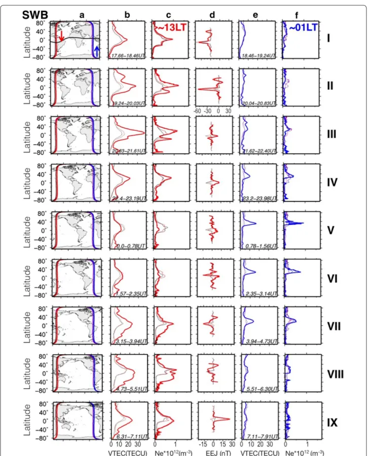
Measurements from the Swarm B satellite were very similar to Swarm A and C results but at ~530 km altitude and in the 01 and 13 LT sectors (Fig. 3). Before the storm and at the initial phase of it, we observe small positive signatures on the dayside, and no significant variations on the nightside (row I). At ~19.2–20.0 UT, the dayside pass revealed a strong VTEC and Ne enhancement at low and mid-latitudes, as well as at high latitudes in the NH (row II, Fig. 3). At 20.8–21.6 UT, the positive dayside storm-time effects further increased up to 40 TECU at low latitudes (row III). One can also notice VTEC and Ne enhancements at high latitudes of the SH, similar to the SWA observations. On the nightside, small storm-time increase in the VTEC occurred at ~21.6–22.4 UT (row III).
At ~22.4–23 UT, both the dayside VTEC and Ne decreased as compared to the previous pass (row IV). At ~23–24 UT, on the nightside, VTEC significantly increased at middle latitudes in the NH (Fig. 3, row IV). The next dayside pass showed a significant drop of the low- and mid-latitude VTEC and Ne as compared to the quiet-time values, indicating the beginning of the negative ionospheric storm at low and partly at mid-dle latitudes (row V). During the next dayside pass, the storm-time Ne value remained below the quiet-time level Ne, while the VTEC started to increase (row VI). On the nightside, strong positive storm was observed at ~0.8– 1.6 UT (row V) and persisted during the next pass at (See figure on previous page.)
Fig. 2 Results from Swarm A a (SWA) on the dayside orbit (ascending, equator crossing at ~11 LT, red curves) and on the nightside orbit
(descend-ing, ~23 LT, blue curves). The VTEC data are shown in columns b and c, the electron density Ne is shown in columns c and f. Column d shows latitu-dinal profiles of the EEJ as obtained from the magnetic data from Swarm and magnetic field models on the dayside orbits (i.e., on the ascending ones). For all parameters, the storm-time values (light thick curves) are compared with the quiet-time values for the day before (thin dark curves). The corresponding satellite trajectories for both the event day and the day before are shown in column a. The UT time of the beginning and ending of the dayside and nightside satellite trajectories is indicated in columns b and e
2.35–3.14 UT (row VI). From 3.15 UT, the dayside VTEC and Ne increased, marking the beginning of the second positive storm (row VII), similarly to the SWA and SWC results. At the same time, the nightside VTEC decreased and the Ne went down to almost undisturbed level (row VII). The next SWB dayside pass showed further increase of the dayside VTEC and Ne throughout the whole SH and exceeded the quiet-time values by 30–500 % (row VIII). From ~6.31 UT, the ionospheric enhancement started to decrease (row IX). On the nightside, from 5.5 to 7.9 UT both VTEC and Ne showed very small values and did not exceed the quiet-time levels.
Comparison of Figs. 2, 3, and 4 reveals that, despite the difference in local times and in the orbital alti-tude between the 2 satellites, the storm-time nightside VTEC increase at SWB is almost as intensive as at SWA and SWC, and reaches ~17–18 TECU. The ionospheric increase in the NH can also be seen in the in situ Ne data; however, it is much less pronounced than in the VTEC. Also, we notice that the maximum nighttime Ne increase at SWB is smaller than that in the SWA and SWC in situ data (Figs. 2, 3, 4, rows III–V). On the dayside, the magni-tude of the positive storm at SWB was slightly larger than at SWA and SWC (Figs. 2, 3, 4, rows II and III) that is, undoubtedly, due to the different local time coverage by these two satellites. The second positive storm phase on the dayside that occurred from ~2.5 to ~6 UT was also captured by all three satellites. However, the nightside response was not the same during this second event.
Column d in Figs. 2, 3, and 4 shows the EEJ magnetic data at ~11 LT (SWA and SWC) and at ~13 LT (SWB) during the main phase of the storm as compared to the quiet-time levels (light thick red lines vs dark thin red and black lines). One can see that with the development of the storm, the EEJ signatures at SWA and SWC first strongly intensified up to −78 nT (at ~19.7 UT, row II), and later, from ~21 UT, they switched from the negative in the main field direction (i.e., eastward) to the positive (i.e., westward), and intensified up to +40 nT (rows III and VI, Figs. 2, 4). At SWB satellite, the EEJ magnitude was slightly smaller, −60 nT and +25 nT, respectively; the latter is, most likely, due to the ~15–20-min time shift in the observations as well as the altitude difference between the satellites. From ~23 UT, the EEJ amplitude diminished at all satellites. Note that the EEJ dynamic behavior is similar at all three satellites, despite the differ-ence in the orbital altitude and local time.
Comparison between the ionospheric and EEJ data from the Swarm constellation leads us to conclusion that variations of the equatorial electric field during the main phase of the June 2015 storm largely contributed in the development of the observed effects in the topside iono-sphere. It is known that on the eastward dayside electric
fields cause the ionospheric uplift and provoke an over-all enhancement of the electron density at low and even mid-latitudes on the dayside (e.g., Tsurutani et al. 2008; Verkhoglyadova et al. 2008). In turn, westward equatorial electric fields are the cause of the downward E × B drifts that weaken the ionospheric fountain effect and provoke the plasma depression.
Figures 2, 3 and 4 show that the dayside positive iono-spheric effects first occurred during the strong eastward EEJ observations (row II). Shortly after the dayside EEJ reversed to westward (~20.0–20.5 UT), a significant ionospheric enhancement was observed on the night-side. However, the next dayside passes of the SWA and SWC, and especially of SWB satellite, show that the dayside VTEC did not change immediately following the reverse of the EEJ: the VTEC first continued to grow (row III), and from ~23 UT it started to significantly decrease and further went below the quiet-time lev-els (rows IV-V). During this time, the nightside Swarm passes showed an extreme increase in the low- and mid-latitude Ne and especially in the VTEC. We explain these latter observations by westward equatorial elec-tric fields that drive the plasma downward on the day-side while, on the nightday-side, they uplift the ionospheric plasma to higher altitudes where the recombination is slower. Our nighttime observations in VTEC are in line with this conclusion. The presence of the enhanced electric fields and, in turn, of the enhanced ExB drift can also be concluded from the observations of fluctu-ations in the electron density (Figs. 2, 4, rows III–IV), which often occur in the post-sunset sector driven by the Rayleigh–Taylor Instability due to the enhanced ExB drift (e.g., Fejer et al. 1999).
Analysis of the ionospheric and the EEJ behavior dur-ing the second sub-phase of the storm (from ~2 UT) demonstrates that the correlation between the EEJ vari-ations and the ionospheric behavior is less obvious than at the beginning of the storm. The EEJ in row VII is espe-cially difficult to explain, as this period of time is charac-terized by a second long-term period of southward IMF Bz and eastward IEF Ey up to ~15 mV/m, that should lead to the PPEF and increase of the EEJ. However, dur-ing this moment of time the EEJ did not exceed −7 to 8 nT in the measurements of all three satellites. One of the possible explanations for that can be in rapid variations of the equatorial currents, so that the satellites fly over the equator at the moment when the EEJ changes from eastward to westward flow. Second, during this period of time the sub-storm activity was less intensive than during the initial phase of the storm, which could play a role on the efficiency of the PPEF. It is known that sub-storms can enhance the PPEF or can serve themselves as a source of PPEF (Huang 2012). Finally, the longitudinal
dependence of the EEJ could have played a role in smaller EEJ values detected by the Swarm satellites.
The second positive storm on the nightside correlates well with a new increase of the counter electrojet, espe-cially in data of SWA and SWC (rows VIII and IX), i.e., in the same manner as during the first sub-event.
Discussions
It is known that storm-time electric fields result from the prompt penetration electric fields (PPEF), driven by the leakage of high-latitude convection electric fields to low latitudes (e.g., Huang et al. 2005; Kikuchi et al. 2008), and by the longer-lived disturbance dynamo electric fields, driven by the storm-time neutral winds through action of the ionospheric dynamo processes (Blanc and Richmond 1980; Maruyama et al. 2007). The PPEF occur during the IMF Bz negative interval, and about 5–12 % of the associated eastward interplanetary electric field (IEF) can penetrate into the ionosphere (e.g., Kelley et al.
2003; Huang et al. 2007; Manoj et al. 2008, 2013; Verk-hoglyadova et al. 2008). A sudden northward Bz turning from steady southward direction can also lead to anoma-lous reversal of the zonal equatorial electric fields (Kelley et al. 1979; Fejer et al. 1979), while the penetration can be as efficient as during Bz negative events (Manoj et al.
2008; Tsurutani et al. 2008). Since the IEF Ey is calculated using the MHD approximation from the IMF Bz and the Vx component of the solar wind speed as –Bz*Vx (http:// omniweb.gsfc.nasa.gov), the northward/positive IMF Bz presumes occurrence of the westward electric fields on the dayside and eastward electric fields on the nightside.
Figure 1b shows that during the main phase of the June 2015 storm the IMF Bz component changed polar-ity several times. Consequently, the IEF Ey followed the oscillatory behavior and varied from −15 to +20 mV/m (Fig. 1b), which is comparable to super-storm values (e.g., Kelley et al. 2003; Huang et al. 2005; Fejer et al. 2007; Balan et al. 2010). It is known that, at the first approxi-mation, the IEF Ey is positively correlated with the zonal equatorial electric field on the local dayside and nega-tively correlated on the local nightside (e.g., Manoj et al.
2008, 2013). Thus, for a positive IEF, the effect on the zonal electric field is primarily eastward during daytime and westward during nighttime. Our observations from Swarm satellites are in agreement with this description and show very good correlation between the EEJ and IEF Ey variations. Comparison of Figs. 1b, 2, 3, and 4
(columns d) reveals that at ~19.0–19.5 UT the EEJ val-ues from the Swarm satellites were largely negative (i.e., eastward, row II in Figs. 2, 3, 4) during the period of the positive (i.e., eastward) IEF Ey values. From ~19.7 UT, the IEF Ey changed to negative (i.e., westward), and remained that almost all the time until ~01 UT of the
next day, except for a short moment of time around 21 UT (Fig. 1b). During this time, we observed largely enhanced positive (westward) EEJ in measurements of all Swarm satellites (Figs. 2, 3, 4, rows III–IV). Swarm showed that the westward EEJ remained enhanced until 22.5–23.0 UT, and then it went back to the quiet-time levels (Figs. 2, 3, 4, rows V–VII).
The rapid oscillations of the IMF Bz and the cor-responding variations of the IEF Ey, most likely, were the reason of the difference in the EEJ measurements between the satellites as was mentioned before. For instance, during the observations of large-amplitude neg-ative EEJ (row II in Figs. 2, 3, 4), SWA and SWC meas-ured the EEJ at ~19.4 UT, i.e., during the maximum of the IEF Ey excursion, while SWB crossed the equator at ~19.7 UT, i.e., when the IEF Ey decreased strongly.
It is important to note that, while the variations of the IMF Bz and IEF Ey continued even at the end of the main phase of the storm (Fig. 1b), we did not observe large lev-els of the EEJ from ~01 UT on June 23, 2015 (Figs. 2, 3, 4, column d, rows VI–VIII).
Following such oscillatory pattern of the equatorial zonal electric fields and the EEJ, the ionospheric behavior during the June 22–23, 2015, storm was also quite vari-able. The PPEF seemed to be the principal driver of the observed extreme Ne and VTEC variations in the top-side ionosphere during the first sub-phase of the storm. In addition to the PPEF, the disturbance dynamo could have increased the effect of penetration of the westward electric fields from ~21 to ~2 UT. It is known that the disturbance dynamo develops over a period of hours and can persist for many hours due to the neutral-air inertia (Maruyama et al. 2007). The effect of the distur-bance dynamo can be especially important on the night-side, since it has been shown that on the nightside both prompt penetration and disturbance dynamo effects are comparable (Maruyama et al. 2007).
During the second sub-phase of the storm, both SWA and SWC showed a short-term but intensive enhance-ment in VTEC and Ne on both day- and night side. SWB showed a large positive storm only on the dayside. From Figs. 2, 3, and 4d, we conclude that these ionospheric alterations do not correlate with the EEJ variations. These observations might indicate that during this sec-ond sub-phase other mechanisms than the PPEF played a role in causing the positive storm effects in the top-side ionosphere. As mentioned before, an increase in the ionospheric electron density or in the VTEC can be also provoked by storm-time-enhanced neutral winds and the consequent ionospheric uplift, by downwelling of the gas due to storm-time-induced thermospheric circula-tion (i.e., increase in the O/N2 ratio), as well as by plasma fluxes from plasmasphere (e.g., Prölss 1995; Danilov
2013). While the neutral winds data are not available, we can analyze the thermospheric O/N2 ratio as meas-ured by the Global Ultraviolet Imager (GUVI) onboard Thermosphere, Ionosphere, Mesosphere Energetics and Dynamics (TIMED) satellite (i.e., Christensen et al.
2003). Additional file 2: Figure S2c shows that on 23 June the O/N2 ratio was largely increased in SH, in particu-lar over Australia and the Indian ocean, as compared to quiet conditions on 21 June (a), and even to the first day of the storm (22 June, b). This O/N2 enhancement is con-sistent with our observations of the positive ionospheric storm in the SH, which also continues until ~6 UT, when the NH Ne experienced a negative storm.
Another interesting feature observed during this storm is the well-pronounced hemispheric asymme-try in the nighttime Ne and VTEC enhancement in both ~23 and 01 LT sectors. The asymmetry is usu-ally explained by the seasonal impact due to the sea-sonal changes in the thermospheric circulation. It is known that in summer the daytime background (solar-induced) circulation is directed equatorwards, and it is poleward in the winter hemisphere (e.g., Fuller-Rowell et al. 1996; Fuller-Rowell 2011). With the onset of a geomagnetic storm, the high-latitude heating drives a global wind surge from both polar regions toward the equator. Consequently, in the summer hemisphere the storm-time daytime circulation coincides with the background one, and it opposes in the winter hemi-sphere. The storm-time changes in the global circula-tion lead to changes in the neutral composicircula-tion and the expansion of the neutral composition bulge to low latitudes (e.g., Fuller-Rowell 2011). On the nightside, the background and the storm-induced circulations are both directed equatorward, which leads to the fact that the composition disturbance can reach much lower latitudes. These storm-time alterations are known to often provoke ionospheric positive storms in the winter hemisphere, whereas negative storms occur more often in the summer hemisphere (e.g., Prölss 1995; Danilov
2013). However, the June 2015 storm occurred just dur-ing the summer solstice time, but we observed stronger effect in the summer hemisphere, which is contrary to the commonly observed features. One can notice in Figs. 2, 3, and 4 that the quiet-time levels also show the hemispheric asymmetry, with slightly larger VTEC and Ne values in the NH (i.e., the summer hemisphere) than in the SH (i.e., the winter hemisphere). This may con-firm the seasonal feature of the observed asymmetry.
It should be noted that, in general, observations of the nighttime positive ionospheric disturbances are suffi-ciently rare and are still difficult to explain (e.g., Tsagouri
et al. 2000). Possible explanation can be in their genera-tion by thermospheric winds before dusk that further rotates on the nightside (Fuller-Rowell et al. 1994). How-ever, in the topside region the positive disturbances can be led by an ionospheric uplift to higher altitudes where the recombination is slower. Previously, Astafyeva et al. (2015a) observed the positive ionospheric disturbance in the topside ionosphere in the summer hemisphere that was explained by a combination of the storm-time PPEF and the enhanced storm-time thermospheric circulation.
Conclusions
By using a set of data from Swarm satellites, we analyzed variations of the ionospheric parameters—VTEC and Ne—in the topside part of the ionosphere during the ini-tial and the main phases of the June 2015 geomagnetic storm. We observed a significant daytime increase in VTEC and Ne at the initial phase of the storm, at ~19– 21 UT, and at the end of the main phase of the storm, at ~3–5 UT on 23 June. One of the most peculiar fea-tures of this storm is the extreme topside increase of the VTEC and the Ne on the nightside (in the ~23 and ~01 LT sectors) in the summer hemisphere that apparently lasted for several hours.
Our analysis of the magnetic data from the Swarm sat-ellites showed very intensive fluctuations of the EEJ dur-ing this storm, which at the beginndur-ing of the main phase of the storm correlated with variations of the Ey com-ponent of the IEF. Comparison of the magnetic EEJ and the ionospheric data variations led us to conclusion that during the first positive phase the storm-time PPEF were the main driver for the observed extreme ionospheric response on the dayside. On the nightside, the topside ionosphere seemed to respond to the combination of the PPEF and the storm-time thermospheric circulation. The disturbance dynamo might have reinforced the effect of the PPEF.
The second sub-phase of the storm was registered from ~2.5 UT and lasted until ~6 UT. Contrary to the first sub-event, the second one was observed at low lati-tudes and in winter hemisphere and seemed to be caused by other drivers than the PPEF. We suggest that the storm-time enhanced thermospheric composition sig-nificantly contributed to the development of this second positive storm.
Our study of the ionospheric response to the June 2015 geomagnetic storm with the additional use of the mag-netic EEJ data demonstrates that the Swarm products can be successfully used for the “full” diagnostics of the near-earth environment and can further be applied for the space weather applications. Having a set of satellite data
is especially useful and important when ground-based data are absent or limited, e.g., in/over the oceans, or in other places with poor instrumentation coverage, which was the case of the June 2015 storm.
It should be noted that for studies of ionospheric vari-ations, data of the thermospheric winds data would be very helpful, but the Swarm satellites are currently at an altitude where the estimation of thermospheric winds is impossible. The thermospheric neutral mass density can be calculated from the accelerometers onboard Swarm satellites (Siemes et al. 2016, current issue), and therefore these data can provide the information about the behav-ior of the neutral component. However, as of today (July 2016) the data are not yet ready to be publicly released (E. Doornbos, private communication, 2016). Future release of those data will make the mission even more accom-plished and successful.
Authors’ contributions
EA has conceived the main idea of this study, has made analysis of the data and has written the first draft of the manuscript. IZ has made data processing for the VTEC data and contributed in the discussions and interpretation of the results as well as in the revision of the draft of the manuscript. PA performed the data processing for the EEJ from the magnetic Swarm data and contrib-uted in the discussion of the results. All authors read and approved the final manuscript.
Author details
1 Institut de Physique du Globe de Paris, Paris Sorbonne Cité, Université Paris
Diderot, UMR CNRS 7154, 35-39 Rue Hélène Brion, Paris 75013, France. 2
Uni-versity of Colorado Boulder, Boulder, CO, USA. 3 National Centers for
Environ-mental Information, Boulder, CO, USA.
Acknowledgements
This work is supported by the European Research Council (ERC Grant Agree-ment No. 307998). We thank the NASA/GSFC’s Space Physics Data Facility’s OMNIWeb service for data of the interplanetary and SYM-H parameters. We are grateful to the ESA EarthNet service for making the Swarm data available (http://earth.esa.int/swarm). We thank Pierdavide Coisson (IPGP) for fruitful discussions. This is IPGP contribution 3779.
Additional files
Additional file 1: Figure S1. The maximum height of the ionospheric F2 layer (HmF2) as measured by COSMIC/F3 mission during the June 22–23, 2015 geomagnetic storm (shown by colored circles). The date and the time period of observations are indicated on the top of each panel. Thin gray circles in each panel show trajectories of SWA satellite during the 2 h of observations, and triangles correspond to the trajectories of SWB. The results show that HmF2 did not exceed 440–450 km, which confirms that the Swarm constellation satellites flew in the topside ionospheric region. Additional file 2: Figure S2. Thermospheric O/N2 ratio as measured by the Global Ultraviolet Imager (GUVI) onboard TIMED satellite on June 21–23, 2015. One can see a significant O/N2 increase in the African, Asian and Australian regions. This increase might have played a role in the posi-tive storm formation over these regions that we observe in the topside ionosphere. The universal time (UT) and the local time (LT) of the equator crossings by the TIMED satellites are shown on the bottom of each panel. The images (a), (b), (c) are downloaded from http://guvitimed.jhuapl.edu.
Competing interests
The authors declare that they do not have competing interests. Received: 5 February 2016 Accepted: 20 August 2016
References
Alken P, Maus S, Vigneron P, Sirol O, Hulot G (2013) Swarm SCARF equato-rial electric field inversion chain. Earth Planet Space 65(11):1309–1317. doi:10.5047/eps.2013.09.008
Alken P, Maus S, Chulliat A, Vigneron P, Sirol O, Hulot G (2014) Swarm equato-rial electric field chain: first results. Geophys Res Lett. doi:10.1002/201 4GL062658
Astafyeva EI (2009) Dayside ionospheric uplift during strong geomagnetic storms as detected by the CHAMP, SAC-C, TOPEX and Jason-1 satellites. Adv Space Res 43:1749–1756. doi:10.1016/j.asr.2008.09.036
Astafyeva E, Zakharenkova I, Doornbos E (2015a) Opposite hemispheric asym-metries during the ionospheric storm of 29–31 August 2004. J Geophys Res 120:697–714. doi:10.1002/2014JA020710
Astafyeva E, Zakharenkova I, Foerster M (2015b) Ionospheric response to the 2015 St. Patrick’s Day storm: a global multi-instrumental overview. J Geo-phys Res Space Phys 120(10):9023–9037. doi:10.1002/2015JA021629
Balan N, Shiokawa K, Otsuka Y, Kikuchi T, Vijaya Lekshmi D, Kawamura S, Yama-moto M, Bailey GJ (2010) A physical mechanism of positive ionospheric storms at low latitudes and midlatitudes. J Geophys Res 115:A02304. doi:
10.1029/2009JA014515
Blanc M, Richmond AD (1980) The ionospheric disturbance dynamo. J Geo-phys Res 85:1669–1686. doi:10.1029/JA085iA04p01669
Buchert S, Zangerl F, Sust M, André M, Eriksson A, Wahlund J-E, Opgenoorth H (2015) SWARM observations of equatorial electron densities and topside GPS track losses. Geophys Res Lett 42:2088–2092. doi:10.1002/2 015GL063121
Christensen AB et al (2003) Initial observations with the Global Ultraviolet Imager (GUVI) on the NASA TIMED satellite mission. J Geophys Res 108(A12):1451. doi:10.1029/2003JA009918
Danilov AD (2013) Ionospheric F-region response to geomagnetic distur-bances. Adv Sp Res 52(3):343–366. doi:10.1016/j.asr.2013.04.019
Fejer BG, Gonzales CA, Farley DT, Kelley MC, Woodman RF (1979) Equatorial electric fields during magnetically disturbed conditions. 1. Effect of the interplanetary magnetic field. J Geophys Res 84(A10):5797–5802 Fejer BG, Scherliess L, de Paula ER (1999) Effects of the vertical plasma drift
velocity on the generation and evolution of equatorial spread F. J Geo-phys Res 104(A9):19859–19869. doi:10.1029/1999JA900271
Fejer BG, Jensen JW, Kikuchi T, Abdu MA, Chau JL (2007) Equatorial ionospheric electric fields during the November 2004 magnetic storm. J Geophys Res 112:A10304. doi:10.1029/2007JA012376
Foster JC et al (2005) Multi-radar observations of the polar tongue of ioniza-tion. J Geophys Res 110:A09S31. doi:10.1029/2004JA010928
Friis-Christensen E, Luehr H, Hulot G (2006) Swarm: a constellation to study the Earth’s magnetic field. Earth Planet Space 58:351–358
Friis-Christensen E, Luehr H, Knudsen D, Haagmans R (2008) Swarm—an earth observation mission investigating geospace. Adv Space Res 41(1):210– 216. doi:10.1016/j.asr.2006.10.008
Fuller-Rowell TJ (2011) Storm-time response of the thermosphere-ionosphere system. In: Abdu MA, Pancheva D, Bhattacharyya A (eds) Aeronomy of the earth’s atmosphere and ionosphere, IAGA Spec. Sopron Book Ser., vol. 2, chapt. 32, pp 419–435, doi:10.1007/978-94-007-0326-1
Fuller-Rowell TJ, Codrescu MV, Moffett RJ, Quegan S (1994) Response of the thermosphere and ionosphere to geomagnetic storms. J Geophys Res 99:3893–3914
Fuller-Rowell TJ, Codrescu MV, Rishbeth H, Moffett RJ, Quegan S (1996) On the seasonal response of the thermosphere and ionosphere to geomagnetic storms. J Geophys Res 101(A2):2343–2353
Goncharenko LP, Foster JC, Coster AJ, Huang C, Aponte N, Paxton LJ (2007) Observations of a positive storm phase on September 10, 2005. J Atmos Solar-Terr Phys 69:1253–1272
Huang C-S (2012) Statistical analysis of dayside equatorial ionospheric electric fields and electrojet currents produced by magnetospheric substorms during sawtooth events. J Geophys Res 117:A02316. doi:10.1029/201 1JA017398
Huang C-S, Foster JC, Kelley MC (2005) Long-duration penetration of the interplanetary electric field to the low-latitude ionosphere during the main phase of magnetic storms. J Geophys Res 110:A11309. doi:10.1029 /2005JA011202
Huang C-S, Sazykin S, Chau JL, Maruyama N, Kelley MC (2007) Penetration electric fields: efficiency and characteristic time scale. J Atm Sol-Terr Phys 69:1135–1146
Kelley MC, Fejer BG, Gonzales CA (1979) An explanation for anomalous equa-torial ionospheric electric fields associated with a northward turning of the interplanetary magnetic field. Geophys Res Lett 6(4):301–304 Kelley MC, Makela JJ, Chau JL, Nicolls MJ (2003) Penetration of the solar wind
electric field into the magnetosphere/ionosphere system. Geophys Res Lett 30(4):1158. doi:10.1029/2002GL016321
Kikuchi T, Hashimoto KK, Nozaki K (2008) Penetration of magnetospheric electric fields to the equator during a geomagnetic storm. J Geophys Res 113:A06214. doi:10.1029/2007JA012628
Lu G, Goncharenko LP, Richmond AD, Roble RG, Aponte N (2008) A dayside ionospheric positive storm phase driven by neutral winds. J Geophys Res 113:A08304. doi:10.1029/2007JA012895
Lühr H, Kervalishvili G, Michaelis I, Rauberg J, Ritter P, Park J, Merayo JMG, Brauer P (2015) The interhemispheric and F region dynamo currents revisited with the Swarm constellation. Geophys Res Lett 42:3069–3075. doi:10.1002/2015GL063662
Manoj C, Maus S, Luhr H, Alken P (2008) Penetration characteristics of the interplanetary electric field to the daytime equatorial ionosphere. J Geophys Res 113:A12310. doi:10.1029/2008JA013381
Manoj C, Maus S, Alken P (2013) Long-period prompt-penetration electric fields derived from CHAMP satellite magnetic measurements. J Geophys Res Space Phys 118:5919–5930. doi:10.1002/jgra.50511
Maruyama N, Richmond AD, Fuller-Rowell TJ, Codrescu MV, Sazykin S, Tof-foletto FR, Spiro RW, Millward GH (2007) Interaction between direct penetration and disturbance dynamo electric fields in the storm-time equatorial ionosphere. Geophys Res Lett 32:L17105. doi:10.1029/200 5GL023763
Olsen N et al (2013) The Swarm Satellite Constellation Application and Research Facility (SCARF) and Swarm data products. Earth Planet Space 65:1189–1200
Pedatella NM, Lei J, Larson KM, Forbes JM (2009) Observations of the ionospheric response to the 15 December 2006 geomagnetic storm: long-duration positive storm effect. J Geophys Res 114:A12313. doi:10.10 29/2009JA014568
Pitout F, Marchaudon A, Blelly P-L, Bai X, Forme F, Buchert SC, Lorentzen DA (2015) Swarm and ESR observations of the ionospheric response to a field-aligned current system in the high-latitude midnight sector. Geo-phys Res Lett. doi:10.1002/2015GL064231
Prölss G (1995) Ionospheric F-region storms. In: Volland H (ed) Handbook of atmospheric electrodynamics, vol 2. CRC Press, Boca Raton, pp 195–248 Siemes C, de Teixeira da Encarnação J, Doornbos E, van den IJssel J, Kraus J,
Pereštý R, Grunwaldt L,Apelbaum G, Flury J, Olsen PEH, (2016) Swarm accelerometer data processing from raw accelerations to ther-mospheric neutral densities. Earth Planet Space 68(1):92. doi:10.1186/ s40623-016-0474-5
Tsagouri I, Belehaki A, Moraitis G, Mavromichalaki H (2000) Positive and nega-tive ionospheric disturbances at middle latitudes during geomagnetic storms. Geophys Res Lett 27(21):3579–3582
Tsurutani BT et al (2008) Prompt penetration electric fields (PPEFs) and their ionospheric effects during the great magnetic storm of 30–31 October 2003. J Geophys Res 113:A05311. doi:10.1029/2007JA012879
Verkhoglyadova OP, Tsurutani BT, Mannucci AJ, Saito A, Araki T, Anderson D, Abdu M, Sobral JHA (2008) Simulation of PPEF effects in dayside low-latitude ionosphere for the October 30, 2003 superstorm. In: Kintner P et al (eds) Mid-latitude ionosphere dynamics and disturbances. AGU, Washington
Yizengaw E, Moldwin MB, Komjathy A, Mannucci AJ (2006) Unusual topside ionospheric density response to the November 2003 superstorm. J Geophys Res 111:A02308. doi:10.1029/2005JA011433
Zakharenkova I, Astafyeva E (2015) Topside ionospheric irregularities as seen from multi-satellite observations. J Geophys Res Space Phys 120:807–824. doi:10.1002/2014JA020330
Zakharenkova I, Cherniak I (2015) How can GOCE and TerraSAR-X contribute to the topside ionosphere and plasmasphere research? Space Weather. doi:
10.1002/2015SW001162
Zakharenkova I, Astafyeva E, Cherniak I (2015) Early morning irregulari-ties detected with space-borne GPS measurements in the topside ionosphere: a multi-satellite case study. J Geophys Res Space Phys 120(10):8817–8834. doi:10.1002/2015JA021447
Zakharenkova I, Astafyeva E, Cherniak I (2016) GPS and in situ Swarm observa-tions of the topside equatorial plasma irregularities. Earth Planet Space 68:1. doi:10.1186/s40623-016-0490-5