Dynamics of Spontaneous (Multi) Centennial‐Scale Variations of the Atlantic Meridional Overturning Circulation Strength During the Last Interglacial

HAL Id: hal-02936233

https://hal.archives-ouvertes.fr/hal-02936233

Submitted on 24 Sep 2020

HAL is a multi-disciplinary open access

archive for the deposit and dissemination of

sci-entific research documents, whether they are

pub-lished or not. The documents may come from

teaching and research institutions in France or

abroad, or from public or private research centers.

L’archive ouverte pluridisciplinaire HAL, est

destinée au dépôt et à la diffusion de documents

scientifiques de niveau recherche, publiés ou non,

émanant des établissements d’enseignement et de

recherche français ou étrangers, des laboratoires

publics ou privés.

Dynamics of Spontaneous (Multi) Centennial-Scale

Variations of the Atlantic Meridional Overturning

Circulation Strength During the Last Interglacial

A. Kessler, N. Bouttes, Didier M. Roche, U. Ninnemann, J. Tjiputra

To cite this version:

A. Kessler, N. Bouttes, Didier M. Roche, U. Ninnemann, J. Tjiputra. Dynamics of Spontaneous

(Multi) Centennial-Scale Variations of the Atlantic Meridional Overturning Circulation Strength

Dur-ing the Last Interglacial. Paleoceanography and Paleoclimatology, American Geophysical Union, 2020,

35 (8), pp.e2020PA003913. �10.1029/2020PA003913�. �hal-02936233�

Overturning Circulation Strength

During the Last Interglacial

A. Kessler1 , N. Bouttes2 , D. M. Roche2,3, U. S. Ninnemann4 , and J. Tjiputra1

1_{Bjerknes Centre for Climate Research, NORCE Norwegian Research Centre, Bergen, Norway,}2_{Laboratoire des Sciences}

du Climat et de l'Environnement, LSCE/IPSL, CEA‐CNRS‐UVSQ, Université Paris‐Saclay, Gif‐sur‐Yvette, France,

3_{Department of Earth Sciences, Vrije Universiteit Amsterdam, Amsterdam, The Netherlands,}4_{Department of Earth}

Science, University of Bergen and Bjerknes Centre for Climate Research, Bergen, Norway

Abstract

Recent reconstructions of bottom water δ13C during the last interglacial (LIG) suggest short‐lived variability in the Atlantic meridional overturning circulation (AMOC). Spontaneous (multi) centennial‐scale variability of the AMOC simulated in the Earth system model of intermediate complexity iLOVECLIM are investigated for that period. The model simulates abrupt AMOC transitions occurring at 300 years frequency and correspond to a switch of the AMOC vigor between a strong (∼17 Sv) and a weak (∼11 Sv) state. The onset of these abrupt transitions is associated with changes in orbital forcings resulting in the decline of summer insolation in the high latitudes of the North Atlantic and affecting the sea ice cover in two key deep convection regions: (1) the northern Nordic Seas (NNS) and (2) the northwest North Atlantic (NWNA). Northward inflow of Atlantic surface water increases the convection depth in (1) and strengthens the Greenland Iceland Norway (GIN) Seas overturning circulation. Subsequent ocean‐atmosphere interactions involving sea ice, ocean heat release, anomalies of evaporation‐precipitation, and wind stress over the Nordic Seas lead also to an increase in deep convection in (2), followed by increase in the AMOC strength.

1. Introduction

Large and abrupt changes in the Atlantic meridional overturning circulation (AMOC) associated with dra-matic climate shifts may have repeatedly occurred during the past Glacial cycle (Rahmstorf, 2002) and have been associated with freshwater input from ice‐rafted detritus into the North Atlantic (Bond & Lotti, 1995; Broecker, 1994; Heinrich, 1988) and disturbances in the North Atlantic Deep Water (NADW) formation (Henry et al., 2016). However, the specific role of icebergs and freshwater forcing in driving the deep circula-tion anomalies is still not resolved (Barker et al., 2015). In contrast, abrupt AMOC variability is less evident during warmer periods such as the late Pleistocene interglacial periods with both model and proxy studies pointing toward a generally vigorous NADW production on millennial and longer time scales (Adkins et al., 1997; Kuhlbrodt et al., 2007; Oppo et al., 1997). The Intergovernmental Panel on Climate Change (IPCC) Assessment Report 2013 and an increasing number of studies (Cheng et al., 2013; Rugenstein et al., 2013; Schmittner et al., 2005; Weaver et al., 2012) conclude that rapid changes in the AMOC are very unlikely to occur by the end of the 21st century, suggesting rather a slow decline from the current state (11% for RCP2.6 and 32% for RCP8.5, in the ensemble means). However, Castellana et al. (2019) evaluate the risk of sudden decline and collapse of the AMOC at 15% and recent studies have revealed bias in the current cli-mate models concerning their AMOC stability. Models have been classified as having either monostable or multistable regimes depending on the sign of their overturning‐related freshwater transport at 30–32°S in the Atlantic (Weaver et al., 2012). Models with different regimes would likely simulate different AMOC responses to a given climate forcing. It is found that a majority of climate models feature an AMOC that imports fresh water into the North Atlantic, that is, monostable (Drijfhout et al., 2011; Weaver et al., 2012), in contrast to observations‐based analysis, which suggest that the current AMOC is in bistable regime (Bryden et al., 2011; Garzoli et al., 2013; McDonagh & King, 2005; Weijer et al., 1999). This means that the ©2020. The Authors.

This is an open access article under the terms of the Creative Commons Attribution License, which permits use, distribution and reproduction in any medium, provided the original work is properly cited.

Key Points:

• Spontaneous (multi)

centennial‐scale variations of the AMOC during the LIG are primarily driven by changes in summer insolation

• Atlantification of the northern Nordic Seas affects the overall AMOC strength through modifications in atmosphere‐ocean dynamics Correspondence to: A. Kessler, auke@norceresearch.no Citation:

Kessler, A., Bouttes, N., Roche, D. M., Ninnemann, U. S., & Tjiputra, J. (2020). Dynamics of spontaneous (multi) centennial‐scale variations of the Atlantic meridional overturning circulation strength during the last interglacial. Paleoceanography and

Paleoclimatology, 35, e2020PA003913. https://doi.org/10.1029/2020PA003913 Received 14 MAR 2020

Accepted 22 JUL 2020

current thermohaline (THC) component of the AMOC, driven by the salinity and temperaturefields, would have multiple modes as it may have had in the past (Rahmstorf, 2002).

In this context, an increasing number of model studies, from the pioneer box model of Stommel (1961) to more recent and complex climate model (Liu et al., 2017; Yin & Stouffer, 2007), have been performed to ana-lyze the capability of climate models to switch from monostable to multistable regimes; highlighting the salt advection feedback as the responsible process for multiple equilibria (Weijer et al., 2019). Other model stu-dies showed that internal processes in the ocean‐atmosphere system could generate spontaneous abrupt var-iations of the AMOC through their influence on the vertical density gradient in the North Atlantic (Arzel et al., 2012; Brown & Galbraith, 2016; Drijfhout et al., 2013; Friedrich et al., 2010; Ganopolski & Rahmstorf, 2001; Peltier & Vettoretti, 2014; Sakai & Peltier, 1997; Schulz et al., 2002; Vettoretti & Peltier, 2015; Winton, 1993). Thus, AMOC oscillations associated with the weak and strong modes of the THC have been analyzed for various climate conditions. However, to the authors knowledge, there have been few efforts to explore the potential for spontaneous changes of the AMOC during warm interglacial boundary conditions. Yet reconstructions reveal that large short‐lived changes in NADW may have been plausible dur-ing this period (Galaasen et al., 2014; Hodell et al., 2009) and potentially the AMOC (Galaasen et al., 2020) may have occurred during the last interglacial period.

Here we use a set of experiments under the last interglacial (LIG) forcing conditions to provide insights into the possible reasons for (multi) centennial oscillations of the AMOC using the Earth system model of inter-mediate complexity (EMIC) iLOVECLIM (Bouttes et al., 2015; Goosse et al., 2010). Specifically, we aim to delineate the thresholds and internal mechanisms within the model responsible for simulating spontaneous, large variations in AMOC strength under the LIG boundary conditions. While Kessler et al. (2020) discuss AMOC‐related changes in ocean carbon cycling, biogeochemistry, and compare to proxy (benthic carbon isotope reconstructions, e.g., Galaasen et al., 2014; Hodell et al., 2009), the internal mechanisms behind these oscillations were not thoroughly evaluated due to the limitation of this previous study design. Here we pro-vide additional experiments in order to delineate the importance of different forcing mechanisms and achieve a mechanistic understanding of the abrupt AMOC variations that could have occurred under the LIG climate conditions. Thus, we use the iLOVECLIM model to provide a dynamically consistent interpre-tation of the mechanisms underlying rapid carbon cycle and climate variability found in recent reconstructions.

2. Method

2.1. Model Description

This study uses the iLOVECLIM model, a carbon isotope‐enabled version of LOVECLIM composed with similar atmosphere, ocean, and vegetation components to that in LOVECLIM version 1.2 (Goosse et al., 2010; Roche et al., 2007). The atmospheric component ECBilt was developed at the Dutch Royal Meteorological Institute (Opsteegh et al., 1998) and has a resolution of 5.6° with three vertical layers at 800, 500, and 200 hPa. The atmosphere is represented by quasi‐geostrophic approximation to which ageos-trophic terms are added in order to better represent the circulation at low latitude, that is, the Hadley cell. The oceanic component CLIO (Coupled Large‐scale Ice Ocean) adopts 20 levels on the vertical coordinate and has a horizontal resolution of∼3°. The oceanic general circulation model (Goosse & Fichefet, 1999) is based on the Navier‐Stokes equations written in a rotating frame of reference including a parameterization for downsloping currents (Campin & Goosse, 1999). This means that shelf water grid box with higher density than the neighboring willflow along the slope until it reaches a depth of equal density while a vertical and horizontal returnflow from the deep ocean to the shelf compensate this volume transport. In addition, the usual approximations are employed such as the hydrostatic and Boussinesq approximations, while an updated version of the thermodynamical sea ice component of Fichefet & Maqueda (1997,1999) is also included. The sea ice growth/decay rates are governed by bottom and surface sea ice prognostic energy bud-gets in leads, where sea ice thickness increases when the snow cover is heavy enough to push the entity under the water level and freeze with the infiltration of seawater. The parameterization of McPhee (1992) is applied for the heatflux from the ocean to the ice and mass conservation controls salt and freshwater sur-face exchanges. The terrestrial biosphere model (VECODE) has three submodels that exchange heat, stress, water, and carbon (Brovkin et al., 1997). Trees and grass are simulated in addition to deserts and subdivided

10.1029/2020PA003913

into four components (leaves, wood, litter, and soil) that exchange carbon, while the fraction of plant functional type (PFT) are computed at equilibrium with the simulated climate. The photosynthesis depends on precipitation, temperature and atmospheric CO2. Finally, the ocean carbon cycle model

applies a nutrient‐phytoplankton‐zooplankton‐detritus (NPZD) model described in Six and Maier‐Reimer (1996) and in addition includes organic and inorganic components as described in Bouttes et al. (2015).

2.2. Experimental Setup

A set of experiments was conducted to study the mechanisms that generate internal (multi) centennial‐scale variability in the AMOC observed in the transient simulation of Kessler et al. (2020) (hereafter referred as

CTRL). We have performed three additional simulations over the 125–115 ka period of the LIG (summarized in Table 1) using prescribed yearly interpolated values of greenhouse gases (CO2, CH4, and N2O) and orbital

forcings from the third phase of the Paleoclimate Modelling Intercomparison Project (PMIP3; https://pmip3. lsce.ipsl.fr/) and compare them to CTRL. The CTRL experiment consists of a transient simulation under nat-ural greenhouse gas and orbital forcings. In the three additional experiments, we repeated the CTRL simula-tion but with (1)fixed greenhouse gases concentration to the value at 125 ka (CO2= 276 ppmv, CH4= 640

ppb, N20 = 263 ppb; this experiment is referred as GHGfixed); (2) prescribed land vegetation to the value at 125 ka (hereafter referred as VEGfixed); and (3)fixed orbital forcings to their values at 125 ka (hereafter referred as ORBfixed. While ORB and GHG experiments allow us to differentiate the influence of orbital and greenhouse gas forcings, respectively, the VEGF experiment allows us to determine the role of the ter-restrial vegetation‐induced climate feedback on the AMOC. The prescribed land vegetation value is taken from a 5,000 years equilibrium simulation under the 125 ka boundary conditions. As in the CTRL experi-ment, these three additional experiments are branched after two consecutive runs in order to set the 125 ka initial conditions; a preindustrial spin‐up followed by an equilibrium experiment using 125 ka boundary conditions. Both experiments are simulated over 5,000 model years and are described in more detail in sec-tion 2.2 of Kessler et al. (2020).

3. Results

3.1. AMOC Response to Varying Forcings

Deep water formation in our model occurs south and north of the Greenland‐Scotland Ridge. The northern formation region is primarily located in the eastern Greenland Iceland Norway (GIN) Sea, while the south-ern formation region is near south Greenland and south of Iceland. We define the AMOC index as the max-imum of the overturning stream function at 27°N. Furthermore, we define the northern branch of the AMOC as the GIN Sea overturning circulation (GSOC) index, which we characterize by the maximum of the overturning stream function north of 70°N. Figure 1 depicts the simulated variations in AMOC (pink) and GSOC (cyan) for the four experiments (CTRL, GHGfixed, VEGfixed, and ORBfixed). The obliquity and June insolation at 60°N forcings are shown in panels (a) and (b) and are decreasing from their maximum values (23.8° and 528.6 W m−2, respectively) toward 115 ka and the Glacial inception.

During thefirst 3,000 years the overturning indices are relatively stable in all experiments after which the model simulates an increase in variability and numerous occurrence of spontaneous (multi) centennial‐scale transitions for the experiments CTRL, GHGfixedand VEGfixed(Figures 1c–1e). In these three experiments, the second half of the LIG is characterized by an AMOC that preferentially operates at a weak

Table 1

Summary of the Different Model Experiments Considered in This Study

Model run Initial conditions Orbital GHG vegetation

CTRL 125 ka equilibrium LIG LIG prognostic

GHG_fixed 125 ka equilibrium LIG fixed prognostic

VEG_fixed 125 ka equilibrium LIG LIG fixed

ORB_fixed 125 ka equilibrium fixed LIG prognostic

Note. The initial conditions for each experiments correspond to the precursor spin‐up at 125 ka boundary conditions itself branched off from a preindustrial 5,000 years spin‐up. The orbital and greenhouse gas (ORB_fixed) forcings denoted by“LIG” refer to natural transient forcings for the LIG period. The vegetation is turned off in the VEGfixedexperiment.

state and abruptly transitions from weak (AMOC∼ 11 Sv and GSOC ∼ 1 Sv) to strong (AMOC ∼ 17 Sv and GSOC∼ 11 Sv) overturning circulation. This result is in line with Friedrich et al. (2010), who used the same atmosphere‐ocean model ECBilt‐CLIO (LOVECLIM) and performed a series of climate sensitivity experiments under preindustrial and intermediate climate ranging between Last Glacial Maximum (LGM

Figure 1. Simulated maximum of Atlantic meridional overturning circulation (AMOC, pink) and GIN Sea overturning

circulation (GSOC, cyan) in Sv (106m3s−1) for indicated experiment (c–f; see Table 1 for explanations). A locally weighted linear regression over 40 years is used and shown by the thick pink and cyan lines. Panel (a) shows the obliquity forcing, and panel (b) depicts the insolation at 60°N during the LIG. The gray shade in panel (c) represents the abrupt transition period analyzed in section 3.3.

10.1029/2020PA003913

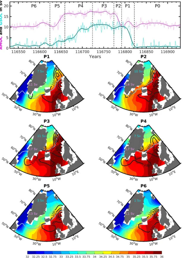
Figure 2. AMOC (pink) and GSOC (cyan) indices in Sv for the CTRL run (top panel) for the time frame 116.930–116.530 (denoted by the gray shade in Figure 1c).

The dashed vertical lines denote averaging intervals for panels P1–P6 of this figure. Panels P1–P6 represent the SSS (shade), the convection depth (black thick lines), the sea ice limit (light blue lines), and the averaged values of the AMOC (pink) and GSOC (cyan) indices for the corresponding intervals.

and) preindustrial boundary conditions. They obtained a similar AMOC behavior in their model experiment when reducing the obliquity from 23.446° to 22.1°. Similar behavior has also been found by Jongma et al. (2007) when applying external freshwater forcings using the ECBilt‐CLIO coupled model. In our simulation, the shift in AMOC variability occurs at a higher obliquity of 23°, which occurs at around 120 ka in CTRL (Figure 1c) and GHGfixed (Figure 1d) experiments and corresponds to a solar insolation at 60°N similar to present day near 460 W m−2(Figure 1b). In VEGfixedthe system is unstable around 120 ka and seems to switch toward a preferentially weak AMOC state later, at around 118.5 ka (Figure 1e) corresponding to an obliquity of about ∼22.8°. In our simulations the initiation and ending of the AMOC/GSOC oscillations show some distinct differences. While the oscillation amplitudes seem to gradually increase in CTRL and VEGfixed (Figures 1c and 1e), they abruptly begin around 120 ka in

Figure 3. Power spectral density for indicated experiment. The orange (blue) lines correspond to thefirst (second) part of

the LIG spanning 125–120 ka (120–115 ka).

10.1029/2020PA003913

GHGfixed(Figure 1d). At the end of the simulations the abrupt variations remain relatively strong in VEGfixed, moderate in GHGfixedwhile they stabilize at weak state in CTRL. No abrupt transitions are simulated for the run only forced by varying greenhouse gases (ORBfixed, Figure 1f), which also show a significant reduction in standard deviation (±1.1 Sv against ±2.5/2.6/2.7 Sv in CTRL/VEGfixed/GHGfixed, respectively). This suggests that the climate generated by the changes in orbital forcings is the main driver for (multi) centennial‐scale variations to occur in our experiments and that these unforced transitions can occur spontaneously (in the model) under LIG climate conditions. Also similar to Friedrich et al. (2010), we note that the changes in GSOC indices are simulated several decades ahead of the AMOC indices (this can be seen in more detail in Figure 2 (top panel) later in the manuscript), suggesting that changes in the GIN Seas are antecedents of the changes south of Greenland (and the global ocean circulation), highlighting the importance of this region as a key area for altering AMOC in the model.

Figure 3 shows the main mode for these abrupt transitions by depicting the power spectral density of the AMOC for each experiment. The LIG is divided into two window periods taking the 120 ka as a pivotal per-iod, which represents a transition for an ocean circulation with a preference for a strong AMOC state to another with a preference for a weak AMOC state. Figure 3 shows that, for experiments CTRL,GHGfixed, and VEGfixed, the second part of LIG (120–115 ka, blue lines) is dominated by these abrupt transitions with a main oscillation frequency of around 300 years per cycle, depicting a power spectrum density up to 10 times stronger as compared to the early LIG window (125–120 ka, red lines). This centennial time scale is similar to that depicted by Friedrich et al. (2010). The experiment withfixed orbital forcing (ORBfixed) shows similar variability in both time windows.

3.2. Regional Deep Convection

Here we only show the analysis over the CTRL experiment, but the same analysis has been performed for the other experiments and revealed similar results. We analyze four domains (NWNA, NENA, SNS, and NNS; see Figure 4 caption for acronyms) in the North Atlantic where deep convection is simulated in our model, influencing the AMOC variations. The regions that simulate the deepest annual average convection depth are in the Nordic Seas with values greater than 300 m depth in SNS and up to 200 m in NNS (Figure 4a). These regions also depict strong interannual variability as illustrated by the contour lines in Figure 4a. The regions south of the Iceland‐Scotland ridge (NWNA and NENA) simulate smaller convection depths, on averaged around 100 m. The NWNA also depicts some considerable variability (up to 100 m depth), while NENA seems to be stable. The time series of convection depth over each region shown in Figure 4b further highlight that two different behaviors are simulated, one depicting changes in convection depth in phase with the changes in AMOC strength (Figure 4b, top panel) while the other is not (Figure 4b, bottom panel). The evolution of the convection depths in NNS and NWNA are characterized by an“on” state mostly simu-lated during thefirst part of the LIG (∼100 m depth) and an “off” state which dominates the late LIG period. The oscillations between one state to the other correspond to the variations depicted by the overturning cir-culation indices (Figure 1c)—strong overturning indices correspond to deeper convection depths. In

Figure 4. (a) Averaged convection depth over the 10,000 years of the CTRL experiment (shaded area). The black thick lines denote the detrended standard

deviation. Four convection areas are identified in our model and are delimited by the colored squares: Northwest North Atlantic (NWNA, in purple), Northeast North Atlantic (NENA, in light orange), Southern Nordic Seas (SNS, in red), and Northern Nordic Seas (NNS, in cyan). The time convection depth time series averaged over each areas are shown in the panel (b) with the corresponding colors.

contrast, the variations of deep convection in NENA and SNS (Figure 4b, red and light orange curves) are in antiphase with the overturning circulation indices; decreasing when the AMOC strengthens. In these regions, the convection remains active during the entire simulation and even increases by twofold in SNS toward 115 ka (Figure 4b, red curve). As a result, the convection occurring in NENA and SNS is mainly suggested to sustain the mean overturning circulation state, as they oscillate between a strong and a weak state (Figure 1c). On the other hand, the NWNA and NNS regions are suggested to mainly contribute to the amplitude of the overturning circulation through enhancement (reduction) of strength during strong (weak) state.

3.3. Physical Ocean Surface Changes

Figures 5 and 6 depict the changes in physical properties at the ocean surface such as the vertical gradient of density over thefirst 600 m (gradρ), the sea surface salinity (SSS), the percentage of sea ice cover, and the sea surface temperature (SST) in each region.

In the regions that show an evolution of convection depth in phase with the overturning indices (NWNA and NNS, Figure 4b, top panel), the early LIG is characterized by a relative low stratification (i.e., Figure 5a) while it is increased by twofold in the late LIG in NWNA and NNS with values around 3 and 2 g m−4, respec-tively. This is consistent with the previously mentioned changes in convection depth occurring in these regions. The changes in SSS (Figure 5b) covary (antiphase) with the vertical stability (r = 0.98) suggesting

Figure 5. Time series of averaged (a) vertical density gradient (Gradρ),(b) sea surface salinity (SSS), (c) sea ice cover in %,

and (d) sea surface temperature (SST) for the CTRL experiment over the Northwest North Atlantic (NWNA, purple thick lines) and Northern Nordic Seas (NNS, cyan thick lines) regions.

10.1029/2020PA003913

that the surface salinity plays a key role in triggering the convection in these regions. In the early LIG relatively high SSS are simulated in NNS and NWNA with values around 34 and 35 psu, respectively. This period corresponds to low sea ice cover (Figure 5c) around 50% in NNS and 10% in NWNA, in the model. High sea ice cover is associated with fresher surface water; hence, when sea ice cover extends, SSS drops, and vice versa. For example, when NNS is fully covered by sea ice (Figure 5c) the SSS is reduced to 33 psu. Here the simulated SST (Figure 5d) is in phase with convection depth and in antiphase with vertical stratification. When the stratification is weak (strong), warmer (colder) SST are simulated. From 125 to 115 ka, the SST declines by about 4°C in both regions and is consistent with the simulated increase of sea ice cover (Figure 5c). However, this cooling does not seem to affect directly (i.e., increase) the convection in these regions, where the influence of surface salinity and fresh water appear dominant.

In regions where the evolution of the convection depth does not correspond to the changes in overturning indices (NENA and SNS, Figure 4b, bottom panel), the vertical stratification (Figure 6a) remains weak dur-ing the entire simulation depictdur-ing values below 1 g m−4. This is consistent with the persistent simulated convection in these regions. Similarly, the simulated SSS (Figure 6b) varies very little and remains above 35 psu, setting favorable conditions for convection to persist. The influence of the sea ice in these regions remains minor as no sea ice is simulated in NENA while it grows only up to 25% of the total area in SNS. As SSS varies little, the changes in convection depth are more affected by the changes in SST (Figure 6d). Consequently, the simulated long‐term surface cooling toward 115 ka (∼2.5°C) in each of these two regions is in good agreement with the slight decreasing trend in vertical stratification (∼0.3 g m−4in 10,000 years, Figure 6a). The increase of the stratification during the abrupt transitions depicted in NENA (Figure 6a)

Figure 6. Similar as Figure 5, but over the Southern Nordic Seas (SNS, red thick lines) and the Northeast North Atlantic

are therefore linked to the increasing SST of about 2°C. No changes in the stratification over the first 600 m are simulated in SNS (Figure 6a, red curve) during the abrupt transitions, where the changes in salinity and temperature seem to balance each other (Figures 7c and 7g).

In our model, the simulated abrupt increases in SSS in the NNS region, are induced by northward intrusion of Atlantic water (more saline) into the GIN Seas also referred to as“Atlantification” of the polar regions, a phenomenon which has been observed in the past decades (Årthun et al., 2012) and is important for setting the boundaries of sea ice in the Barents Sea. As this region becomes fresher toward 115 ka, the intrusion of saline Atlantic surface water generates even larger modifications. This sudden increase in SSS generates deep convection in NNS and in the regions south of Greenland (NWNA) few decades later. The complete set of processes linking NNS to NWNA will be discussed in section 3.5. On the other hand, the NENA and SNS regions depict, in general, higher mean surface salinity and appear to be more resilient to the climate evolution over the simulation period, with a higher influence from changes in surface temperature than changes in surface salinity.

3.4. Role of Summer Air Temperature

The high‐latitude cooling toward 115 ka appears to be a key factor for initiating the high‐frequency AMOC transitions at the mid‐LIG. This cooling is particularly important during the summer as it modulates the melting season of the sea ice and consequently the remaining total sea ice cover during the deep convection season (winter). Figure 8 shows the time series of summer air temperature over the latitude bands 69–80°N and depicts a general and persistent cooling in all of the experiments that exhibit abrupt AMOC variations (CTRL, GHGfixed, and VEGfixed). The CTRL and GHGfixedexperiments (Figure 8, black and light blue lines) simulate relatively similar summer temperature where GHGfixed is only 0.3°C warmer during weak AMOC states at the end of the LIG. This may be due to the small difference in atmospheric CO2

concentra-tion used in the radiative budget calculaconcentra-tion. Indeed, at the end of the LIG the constant value of atmospheric CO2used in GHGfixedis slightly higher (up to 10 ppm) than the one used in CTRL (prescribed values from PMIP3). The VEGfixedexperiment is, in general, warmer than CTRL and GHGfixed. Consequently, the oscilla-tions are delayed until around 118.5 ka. The temperature in ORBfixedremains relatively stable and warm dur-ing the entire simulation period, allowdur-ing most of the sea ice produced in the winter to melt durdur-ing the

Figure 7. Vertical profiles of regional anomalies of (a–d) temperature and (e–h) salinity for each phase P1–P6 relative to

P0. The average is calculated over each region (a, e) NNS, (b, f) NWNA, (c, g) SNS, and (d, h) NENA.

10.1029/2020PA003913

summer. Notably, in each experiment with high AMOC variability (CTRL, GHGfixed, and VEGfixed) the pronounced AMOC oscillatory state begins in each case around the time period when summer temperature decreases to roughly−4°C at 75°N. This occurs slightly before 120 ka in CTRL and GHGfixed and later at 118.5 ka in VEGfixeddue to the higher temperatures in this simulation. This threshold marks the limit below which the summer sea ice does not melt in response to the atmospheric forcing and is therefore only affected by water mass changes. This confirms that the NNS, which is the most impacted by sea ice cover, is the key region for initiating the high‐frequency AMOC variations in the model. Our model simulations demonstrate the key role of air temperature in establishing the seasonal sea ice cov-erage and consequently the timing of AMOC phase transition. Figure 9 highlights for each experiment the mean seasonal air temperature at 75°N at both the beginning and end of the large AMOC oscillation phase. The CTRL experiment simulates the coldest seasonal cycle at both the onset of the oscillations and at the end of the LIG (Figure 9, black solid and dashed lines). The GHGfixedand VEGfixedexperiments are on averaged warmer than CTRL by 1°C and 3.6°C, respectively. As previously mentioned, the warmest period (July) remains below−4°C. The gray shading (Figure 9) highlights the range of temperatures for which abrupt transitions are simulated in our experiments. Above this range, the atmospheric temperature is warm enough during the summer to considerably reduce the summer sea ice extent and therefore the averaged sea ice extent over the year. With a retreated sea ice, more Atlantic water is able to penetrate into the north-ern Nordic Seas and south of Greenland increasing the surface salinity (Figure 5b) and setting the AMOC into its strong state. While the initiation of the AMOC oscillation seems to be linked to a cold enough climate for pushing the system into its weak state, the termination period of the large oscillations phases remains less clear. Do the oscillations stop as suggested by the CTRL run (Figure 1c) or do they just become less frequent as the climate continues to cool down? One hypothesis could be that the sea ice becomes too thick to be melted only by ocean heatflux. The sea ice is indeed approximately 10 to 15 cm thicker in CTRL than in GHGfixed. Additional experiment on sea ice and ocean heatflux sensitivity would be needed to give more insight into the long‐term AMOC stability beyond our experimental period.

3.5. Centennial‐Scale AMOC Variability and Mechanisms

In the previous subsections, we highlight that changes in GSOC are antecedent to changes (increase) in total AMOC which are associated to greater convection depth south of Greenland (also defined here as the NWNA region). In this subsection, we connect the processes occurring in the NNS region, that are responsible for the simulated increase in GSOC indices, to the changes occurring in NWNA and in AMOC indices. To do so we show the example of the last oscilla-tion of the CTRL run (Figure 1c, gray shade), which we divide into several phases. Figures , 2,10, and 11 illustrate atmosphere‐ocean

Figure 9. Seasonal air temperature averaged over 1,000 years around 116.5 ka

(beginning of AMOC oscillations, thick lines) and 119.5 ka* (end of AMOC oscillations in CTRL, dashed lines). The gray‐shaded area represents the range of simulated seasonal air temperature to which abrupt transitions in AMOC are depicted.

interactions during each of these phases and Figure 11 shows the evolution of the temperature (T) and salinity (S) vertical profiles in each of the four regions presented in Figure 4a.

The phase“P0” (Figure 2, top panel) corresponds to a weak AMOC state characterized by an extended sea ice cover over NNS and NWNA comparable to what is simulated during P6 (Figure 2, P6, light blue line). During this phase, heat accumulates in NNS below 200 m depth as the sea ice covers up to 100% of the region redu-cing the heatflux toward the atmosphere. This process weakens the stratification of the water column,

Figure 10. Anomalies evaporation‐precipitation (E‐P) in cm yr−1(shade) and air temperature in °C (contour lines) for each of the phases described in Figure 2 (top panel). These anomalies take the interval P0 for reference. P6 does not depict any significant changes in air temperature as compared to P0.

10.1029/2020PA003913

preconditioning the NNS region for deep convection. Thefirst phase (P1) is characterized by the activation of deep convection in NNS (Figure 2, P1). It is initiated by the inflow of saline (>34.75 psu) and warm Atlantic surface waters, which abruptly increase the SSS in this region by 1 psu (Figure 7e) and the SST by 2°C (Figure 7a). The SSS increase overwhelms the SST increase, therefore the convection starts and GSOC index increases (7 Sv). Phase 2 (P2) is characterized by a reduced sea ice cover induced by both the advection of warm Atlantic surface waters and the mixing of the interior ocean heat. As a result, more heat escapes from the ocean to the atmosphere generating a positive anomaly in air temperature up to +10°C over the NNS (Figure 10, P2, green contours). Associated to the increase in surface air

Figure 11. Anomalies wind stress in N m−2(shade) and its direction (arrows) for each of the phases described in Figure 2 (top panel). These anomalies take the interval P0 for reference.

temperature, the model simulates an increase in evaporation‐precipitation (E‐P, Figure 10, shade), which gradually extends southward toward the NWNA region. This surface flux response acts as a positive feedback further increasing the surface salinity in both regions, although the largest positive SSS anomalies occur in regions where the fraction of high‐salinity Atlantic water increases. The warm anomaly generates a modification in the wind stress (Figure 11, P2–P4) increasing the easterlies flow south of Iceland and advecting more Atlantic waters toward the NWNA. Consequently, both the E‐P and the Atlantic water influx increase the SSS in NWNA by up to 1.5 psu (Figure 7f) in P3 relative to P0 and the convection depth deepens. This gradually strengthens the total AMOC, which reaches its maximum in P3 (17 Sv, Figure 2, P3). Hence, P3 is characterized by both maximum AMOC and GSOC strengths, which lasts for about 50 years. The exact reason for this time scale remains difficult to determine, however, a per-sistent AMOC‐induced northward freshwater transport at 33° (∼0.3 Sv) sets the model simulations in a monostable regime. This freshwaterflow increases by about 0.05 Sv when the AMOC strengthens, slowly acting as a restoring force (e.g., Liu et al., 2013,2015). As a result, GSOC strength begins to decline in P4 (Figure 2, P4) and the associated heat loss in the NNS reduces. We note that the temperature below 200 m depth in NNS decreases by about 2°C between the beginning of P1 to the end of P3 (Figure 7a). This cooling could also negatively affect the magnitude of the heat loss toward the atmosphere and impact the time scale of AMOC recovery. The air temperature anomaly diminishes over the NNS from 10 to 4°C (Figure 10, P4), and the sea ice formation gradually returns contributing to the surface freshening (Figure 7e). The convec-tion in the NWNA remains active for the proceeding 60 years as the anomaly of salinity remains high (Figure 7f). This is the result of both persistent strong anomalies of wind stress (Figure 11, P4) and E‐P (Figure 10, P4) near Greenland, responding to the remaining +6°C air temperature anomaly (Figure 10, P4). In phase 5 (P5), the salinity anomaly continues to reduce in the NNS area (/sim0.4 psu) with a complete return of the sea ice and GSOC declines to 3 Sv. At this point, the anomalously warm air temperature as well as the induced wind stress anomalies over the entire North Atlantic disappear. Finally, the sea ice starts to regrow in the NWNA region. The AMOC strength declines toward its weak state (13 Sv). In phase 6 (P6), the

Figure 12. Diagram summarizing the processes affecting the AMOC stability. The following abbreviations are used: air

temperature (Ta), freshwater (FW), and Atlantic waters (AW).

10.1029/2020PA003913

total AMOC returns to its weak state (11 Sv) and the GSOC is almost shut down (1 Sv) as the Atlantic surface waters retreated further south, leaving the NNS and NWNA regions covered by sea ice and fresher surface water.

Figure 7 allows us to further analyze the effect of the temperature and salinity regarding each region. The NNS and NWNA regions depict near‐surface salinity changes of about 1.5 psu (Figures 7e and 7f) which overwhelm the associated temperature increase (Figures 7a and 7b) and control the activation of the deep convection. On the other hand, SNS and NENA depict stronger changes in temperature (Figures 7c and 7d, up to 3.8°C) relative to salinity (Figures 7g and 7h, only 0.5 psu maximum), which sets the temperature as main driver for deep convection in these regions. This is slightly less pronounced in NENA where the anomalies in both temperatures and salinity are smaller.

4. Discussion and Conclusion

We investigated the mechanisms responsible for plausible spontaneous (multi) centennial‐scale AMOC shifts in the iLOVECLIM model under the LIG boundary conditions. Ourfindings reveal that abrupt transi-tions of the AMOC from strong to weak states may also have been plausible during the LIG under natural greenhouse gas and orbital forcings. These AMOC shifts are comparable in time scale to that suggested by proxy marine records from that period (Galaasen et al., 2014, 2020; Hodell et al., 2009), which have been interpreted as modifications of deep water mass geometry and potentially AMOC strength (Kessler et al., 2020).

The two simulated AMOC states are characterized by the activation and deactivation of deep convection areas in (i) the northern Nordic Seas (NNS) followed several decades later by changes in (ii) the Northwest North Atlantic (NWNA). These (de)activations modulate the AMOC strength and are shown to be associated with the alteration of the vertical stratification due to salinity/fresh water influence. In our model, the changes in water mass stability is initially driven by the growing presence of sea ice, which hin-ders the“Atlantification” process (advection of warm and saline surface water) into the NNS and NWNA regions. The major role of the salinity/fresh water depicted by our study in affecting the vertical stability has also been shown in previous studies applying ECBilt‐CLIO coupled model (Jongma et al., 2007; Schulz et al., 2007) and LOVECLIM (Friedrich et al., 2010). Although the AMOC oscillations in Jongma et al. (2007) arise from external fresh water forcing into the Labrador Sea, the general processes are still similar to those found in our study with a change in surface salinity/fresh water into this region (here approximately corresponding to NWNA) strongly modifies the AMOC strength and can occur spontaneously in the model under LIG boundary conditions.

In this study, the decrease of high‐latitude insolation, primarily due to the declining obliquity, is critical for initiating the (multi) centennial‐scale oscillations of the AMOC strength. These variations occur effectively as jumps between weak (∼11 Sv) and strong (∼17 Sv) AMOC states. As insolation declines there is a gradu-ally increasing preference toward the AMOC weak state with less frequent episodes of strong AMOC. We found a common threshold to all our experiments depicting spontaneous AMOC strength variations (CTRL,GHGfixed, and VEGfixed): ∼ −4°C in summer's (JJA) air temperature over the latitude bands 69– 80°N. We suggest that below that temperature, the sea ice only responds to changes in surface water tem-perature (i.e., advection of warm Atlantic surface water) as the atmosphere is cold enough to maintain the sea ice cover. Consequently, the annual sea ice extends abruptly in NNS and NWNA, lowering the SSS and reducing the deep convection in these regions, and thereby altering GSOC and AMOC. Yet it is not clear if with further cooling, the oscillations of the AMOC would stop (as suggested by CTRL experiment) or become more rare as it would demand more energy from the ocean to melt a thicker sea ice cover. We note that Bakker et al. (2013) also reported an abrupt decrease of the AMOC strength around 120 ka in their LIG experiment with the LOVECLIM model. However, they linked it to a sudden decrease of January's air tem-perature over the latitude bands 60–90°N. In our simulations, a similar cooling is simulated during the win-ter months (DJF, 7°C, not shown here) when the AMOC starts to oscillate, but it warms back up to its previous value until the next abrupt transition. On the contrary, the summer temperature (JJA) shows less variability which is the reason why we suggest it as a crucial threshold. We note that the July air temperature in Bakker et al. (2013) seems also to be slightly above−4°C when the AMOC abruptly weakens, which is consistent with ourfinding.

We show that internal processes in the atmosphere‐ocean system, strongly supported by the presence of sea ice, trigger the simulated abrupt transitions. First, the sea ice presence in key convection regions initiates the AMOC swings by turning off the convection. When the NNS is fully covered by sea ice, heat accumulates below 200 m depth for up to 150 years (Figure 12). This heat corresponds to an average temperature increase of about 2°C, which helps destabilizing the stratification and creating a precondition for deep convection in the NNS region. Friedrich et al. (2010) suggested the deep decoupling as the trigger for deep convection, while it is not the case in our study. In their study, this arose from a subsurface temperature increase of about 4°C which is stronger than what is simulated in our study. Our results support the idea that the main trigger affecting the convection regions remains the changes in salinity/fresh water occurring in the upper ocean layers. Here, we refer to this generically as the relative influence of Atlantic surface waters in NNS and NWNA, although E‐P feedbacks enhance the initial changes. We note that this advection of saline Atlantic water seems to dominate over the potential contribution of Arctic sea ice melt as shown in Figure 2, P1 and P2 where the SSS still increases in NNS while the sea ice melts. Second, the∼25 years delay between the variations in GSOC and AMOC emanates from a series of ocean‐atmosphere processes (namely, ocean heat release—anomalously warmer air temperature—southerly increase in the Denmark Strait— advection of warmer Atlantic surface water) that link the NNS and NWNA regions and ultimately result in reduced sea ice extent around Greenland. Finally, we suggest that the monostable regime of our model simulation, and its negative feedback on the AMOC increase, provides a potential restoring force, assisted by the reduction of oceanic heat release from the NNS region as the temperature below 200 m decreases by about 2°C. These processes are summarized in Figure 12 and correspond relatively well to that described for the LOVECLIM model in Friedrich et al. (2010) even though the AMOC strength they simulated is more than 50% stronger than in our study and that the abrupt AMOC transition they described is on the opposite sign as the one described here (i.e., they showed reduction, whereas we show increase in AMOC strength). This suggests that for a certain range of AMOC state, the model is able to generate spontaneous and large variations in AMOC involving changes in both strength and structure of the overturning. This higher‐instability regime arises suddenly under the influence of gradual forcing due to key nonlinearities in the response to this gradual forcing.

This study shows the importance of the sea ice cover in the high latitudes and how the ocean‐atmosphere system can trigger short‐lived climate transitions and link two regions of high importance for the over-turning circulation. While the warmer (early) part of the LIG remains stable, it seems that there is a threshold when the sea ice has extended further southward to feedback on the atmospheric temperature and ocean heat content. We suggest that such mechanisms could have been involved during the late LIG, for instance around the 119 ka event reported in Galaasen et al. (2014), where no ice rafted detritus could be linked to the large variations inδ13C, which suggest the possibility that a large water mass reorganiza-tion occurred. These mechanisms could also be potential candidates for the shifts recorded during pre-vious interglacials such as the MIS 11c and MIS 9e, where both occur while the IRD record is low (Galaasen et al., 2020). Further model analysis under previous interglacial boundary conditions are required to test the range of background conditions, especially in sea ice extent, capable of triggering such variability/instability.

In addition, setting these spontaneous AMOC variations into a broader context, we note that no significant changes in SSTs are simulated in the Atlantic section of the Southern Ocean (not shown here) when the AMOC switches from one operating mode to another. This potentially distinguishes the centennial AMOC oscillations simulated in this study from the multimillennial AMOC oscillations of glacial periods (Broecker, 1997; Toggweiler & Lea, 2010). Furthermore, the key regions in this model (NNS and NWNA) where sea ice, surface oceanfluxes, and water mass advection changes are crucial for setting the vertical stra-tification and the overturning strength are projected to be ice free as early as the second half of this century. This suggests that such mechanisms responsible for the increase in AMOC strength are unlikely to occur toward the end of this century.

Conflict of Interest

The authors declare no conflict of interest.

10.1029/2020PA003913

Data Availability Statement

The model data are available on the Norwegian Research Data Archive server (https://doi.org/10.11582/ 2019.00037, Kessler, 2019 and https://doi.org/10.11582/2020.00033, Kessler, 2020).

References

Adkins, J. F., Boyle, E. A., Keigwin, L., & Cortijo, E. (1997). Variability of the North Atlantic thermohaline circulation during the last interglacial period. Nature, 390(6656), 154. https://doi.org/10.1038/36540

Årthun, M., Eldevik, T., Smedsrud, L. H., Skagseth, O., & Ingvaldsen, R. B. (2012). Quantifying the influence of Atlantic heat on Barents sea ice variability and retreat. Journal of Climate, 25(13), 4736–4743. https://doi.org/10.1175/JCLI-D-11-00466.1

Arzel, O., England, M. H., de Verdiere, A. C., & Huck, T. (2012). Abrupt millennial variability and interdecadal‐interstadial oscillations in a global coupled model: Sensitivity to the background climate state. Climate Dynamics, 39(1‐2), 259–275. https://doi.org/10.1007/s00382-011-1117-y

Bakker, P., Stone, E. J., Charbit, S., Groeger, M., Krebs‐Kanzow, U., Ritz, S. P., et al. (2013). Last interglacial temperature evolution—A model inter‐comparison. Climate of the Past, 9, 605–619. https://doi.org/10.5194/cp-9-605-2013

Barker, S., Chen, J., Gong, X., Jonkers, L., Knorr, G., & Thornalley, D. (2015). Icebergs not the trigger for North Atlantic cold events. Nature,

520(7547), 333–336. https://doi.org/10.1038/nature14330

Bond, G. C., & Lotti, R. (1995). Iceberg discharges into the North Atlantic on millennial time scales during the last glaciation. Science,

267(5200), 1005–1010. https://doi.org/10.1126/science.267.5200.1005

Bouttes, N., Roche, D. M., Mariotti, V., & Bopp, L. (2015). Including an ocean carbon cycle model into iLOVECLIM (v1. 0),. Geoscientific

Model Development, 8, 1563–1576. https://doi.org/10.5194/gmd-8-1563-2015

Broecker, W. S. (1994). Massive iceberg discharges as triggers for global climate change. Nature, 372(6505), 421–424. https://doi.org/ 10.1038/372421a0

Broecker, W. S. (1997). Thermohaline circulation, the achilles heel of our climate system: Will man‐made CO2upset the current balance?

Science, 278(5343), 1582–1588. https://doi.org/10.1126/science.278.5343.1582

Brovkin, V., Ganopolski, A., & Svirezhev, Y. (1997). A continuous climate‐vegetation classification for use in climate‐biosphere studies.

Ecological Modelling, 101(2‐3), 251–261. https://doi.org/10.1016/S0304-3800(97)00049-5

Brown, N., & Galbraith, E. D. (2016). Hosed vs. unhosed: Interruptions of the Atlantic meridional overturning circulation in a global coupled model, with and without freshwater forcing. Climate of the Past, 12(8), 1663–1679. https://doi.org/10.5194/cp-12-1663-2016 Bryden, H. L., King, B. A., & McCarthy, G. D. (2011). South Atlantic overturning circulation at 24 s. Journal of Marine Research, 69(1),

38–55. https://doi.org/10.1357/002224011798147633

Campin, J.‐M., & Goosse, H. (1999). Parameterization of density‐driven downsloping flow for a coarse‐resolution ocean model in z‐ coordinate. Tellus A, 51(3), 412–430. https://doi.org/10.1034/j.1600-0870.1999.t01-3-00006.x

Castellana, D., Baars, S., Wubs, F. W., & Dijkstra, H. A. (2019). Transition probabilities of noise‐induced transitions of the Atlantic Ocean circulation. Scientific Reports, 9(1), 1–7. https://doi.org/10.1038/s41598-019-56435-6

Cheng, W., Chiang, J. C. H., & Zhang, D. (2013). Atlantic meridional overturning circulation (AMOC) in CMIP5 models: RCP and historical simulations. Journal of Climate, 26(18), 7187–7197.

Drijfhout, S., Gleeson, E., Dijkstra, H. A., & Livina, V. (2013). Spontaneous abrupt climate change due to an atmospheric blocking–sea‐ice– ocean feedback in an unforced climate model simulation. Proceedings of the National Academy of Sciences, 110(49), 19,713–19,718. https://doi.org/10.1073/pnas.1304912110

Drijfhout, S., Weber, S. L., & van der Swaluw, E. (2011). The stability of the MOC as diagnosed from model projections for pre‐industrial, present and future climates. Climate Dynamics, 37(7‐8), 1575–1586. https://doi.org/10.1007/s00382-010-0930-z

Fichefet, T., & Maqueda, M. A. M. (1997). Sensitivity of a global sea ice model to the treatment of ice thermodynamics and dynamics.

Journal of Geophysical Research, 102(C6), 12,609–12,646. https://doi.org/10.1029/97JC00480

Fichefet, T., & Maqueda, M. M. (1999). Modelling the influence of snow accumulation and snow‐ice formation on the seasonal cycle of the Antarctic sea‐ice cover. Climate Dynamics, 15(4), 251–268. https://doi.org/10.1007/s003820050280

Friedrich, T., Timmermann, A., Menviel, L., Elison Timm, O., Mouchet, A., & Roche, D. M.(2010). The mechanism behind internally generated centennial‐to‐millennial scale climate variability in an earth system model of intermediate complexity. Geoscientific Model

Development, 3(2), 377–389. https://doi.org/10.5194/gmd-3-377-2010

Galaasen, E. V., Ninnemann, U. S., Irvalı, N., Kleiven, H. K. F., Rosenthal, Y., Kissel, C., & Hodell, D. A. (2014). Rapid reductions in North Atlantic deep water during the peak of the last interglacial period. Science, 343(6175), 1129–1132. https://doi.org/10.1126/

science.1248667

Galaasen, E. V., Ninnemann, U. S., Kessler, A., Irvalı, N., Rosenthal, Y., Tjiputra, J., et al. (2020). Interglacial instability of North Atlantic deep water ventilation. Science, 367(6485), 1485–1489. https://doi.org/10.1126/science.aay6381

Ganopolski, A., & Rahmstorf, S. (2001). Rapid changes of glacial climate simulated in a coupled climate model. Nature, 409(6817), 153–158. https://doi.org/10.1038/35051500

Garzoli, S. L., Baringer, M. O., Dong, S., Perez, R. C., & Yao, Q. (2013). South Atlantic meridionalfluxes. Deep Sea Research Part I:

Oceanographic Research Papers, 71, 21–32. https://doi.org/10.1016/j.dsr.2012.09.003

Goosse, H., Brovkin, V., Fichefet, T., Haarsma, R., Huybrechts, P., Jongma, J., et al. (2010). Description of the earth system model of intermediate complexity LOVECLI M version 1.2. Geoscientific Model Development, 3, 603–633. https://doi.org/10.5194/gmd-3-603-2010

Goosse, H., & Fichefet, T. (1999). Importance of ice‐ocean interactions for the global ocean circulation: A model study. Journal of

Geophysical Research, 104(C10), 23,337–23,355. https://doi.org/10.1029/1999JC900215

Heinrich, H. (1988). Origin and consequences of cyclic ice rafting in the northeast Atlantic Ocean during the past 130,000 years. Quaternary

Research, 29(2), 142–152. https://doi.org/10.1016/0033-5894(88)90057-9

Henry, L. G., McManus, J. F., Curry, W. B., Roberts, N. L., Piotrowski, A. M., & Keigwin, L. D.(2016). North Atlantic ocean circulation and abrupt climate change during the Last Glaciation. Science, 353(6298), 470–474. https://doi.org/10.1126/science.aaf5529

Hodell, D. A., Minth, E. K., Curtis, J. H., McCave, I. N., Hall, I. R., Channell, J. E. T., & Xuan, C.(2009). Surface and deep‐water hydrography on gardar drift (Iceland basin) during the last interglacial period. Earth and Planetary Science Letters, 288(1‐2), 10–19. https://doi.org/ 10.1016/j.epsl.2009.08.040

Acknowledgments

This work was supported by the Research Council of Norway funded project THRESHOLDS (254964) and ORGANIC (239965) and Bjerknes Centre for Climate Research project BIGCHANGE. We acknowledge the Norwegian Metacenter for Computational Science and Storage Infrastructure (Notur/Norstore) Projects nn1002k and ns1002k for pro-viding the computing and storing resources essential for this study. We thank Xu Zhang and anonymous reviewer for their constructive feed-backs. We also thank Matthew Huber for the time he dedicated in processing our manuscript and his additional feedback. J. T. also acknowledges funding from Research Council of Norway (Columbia, 275268).

Jongma, J. I., Prange, M., Renssen, H., & Schulz, M. (2007). Amplification of Holocene multicentennial climate forcing by mode transitions in North Atlantic overturning circulation. Geophysical Research Letters, 34, L15706. https://doi.org/10.1029/2007GL030642

Kessler, A. (2019). Lig_transient_125ka‐115ka [data set]. Norstore. https://doi.org/10.11582/2019.00037 Kessler, A. (2020). Lig_transient_forcing_experiment [data set]. Norstore. https://doi.org/10.11582/2020.00033

Kessler, A., Bouttes, N., Roche, D. M., Ninnemann, U. S., Galaasen, E. V., & Tjiputra, J. (2020). Atlantic meridional overturning circulation andδ13C variability during the last interglacial. Paleoceanography and Paleoclimatology, 35(5), e2019PA003818.

Kuhlbrodt, T., Griesel, A., Montoya, M., Levermann, A., Hofmann, M., & Rahmstorf, S. (2007). On the driving processes of the Atlantic meridional overturning circulation. Reviews of Geophysics, 45, RG2001. https://doi.org/10.1029/2004RG000166

Liu, W., Liu, Z., Cheng, J., & Hu, H. (2015). On the stability of the Atlantic meridional overturning circulation during the last deglaciation.

Climate Dynamics, 44(5‐6), 1257–1275. https://doi.org/10.1007/s00382-014-2153-1

Liu, W., Liu, Z., & Hu, A. (2013). The stability of an evolving atlantic meridional overturning circulation. Geophysical Research Letters, 40, 1562–1568. https://doi.org/10.1002/grl.50365

Liu, W., Xie, S.‐P., Liu, Z., & Zhu, J. (2017). Overlooked possibility of a collapsed Atlantic meridional overturning circulation in warming climate. Science Advances, 3(1), e1601666. https://doi.org/10.1126/sciadv.1601666

McDonagh, E. L., & King, B. A. (2005). Oceanicfluxes in the South Atlantic. Journal of Physical Oceanography, 35(1), 109–122. https://doi. org/10.1175/JPO-2666.1

Oppo, D. W., Horowitz, M., & Lehman, S. J. (1997). Marine core evidence for reduced deep water production during termination iI followed by a relatively stable substage 5e (Eemian). Paleoceanography, 12(1), 51–63. https://doi.org/10.1029/96PA03133

Opsteegh, J. D., Haarsma, R. J., Selten, F. M., & Kattenberg, A. (1998). ECBILT: A dynamic alternative to mixed boundary conditions in ocean models. Tellus A: Dynamic Meteorology and Oceanography, 50(3), 348–367. https://doi.org/10.3402/tellusa.v50i3.14524 Peltier, W. R., & Vettoretti, G. (2014). Dansgaard‐Oeschger oscillations predicted in a comprehensive model of glacial climate: A “kicked”

salt oscillator in the Atlantic. Geophysical Research Letters, 41, 7306–7313. https://doi.org/10.1002/2014GL061413

Rahmstorf, S. (2002). Ocean circulation and climate during the past 120,000 years. Nature, 419(6903), 207. https://doi.org/10.1038/ nature01090

Roche, D. M., Dokken, T. M., Goosse, H., Renssen, H., & Weber, S. L. (2007). Climate of the Last Glacial Maximum: sensitivity studies and model‐data comparison with the LOVECLIM coupled model. Climate of the Past, 3, 205–224. https://doi.org/10.5194/cp-3-205-2007 Rugenstein, M. A. A., Winton, M., Stouffer, R. J., Griffies, S. M., & Hallberg, R. (2013). Northern high‐latitude heat budget decomposition

and transient warming. Journal of Climate, 26(2), 609–621.

Sakai, K., & Peltier, W. R. (1997). Dansgaard–Oeschger oscillations in a coupled atmosphere–ocean climate model. Journal of Climate,

10(5), 949–970. https://doi.org/10.1175/1520-0442(1997)010<0949:DOOIAC>2.0.CO;2

Schmittner, A., Latif, M., & Schneider, B. (2005). Model projections of the North Atlantic thermohaline circulation for the 21st century assessed by observations. Geophysical Research Letters, 32, L23710. https://doi.org/10.1029/2005GL024368

Schulz, M., Paul, A., & Timmermann, A. (2002). Relaxation oscillators in concert: A framework for climate change at millennial timescales during the Late Pleistocene. Geophysical Research Letters, 29(24), 46–1. https://doi.org/10.1029/2002GL016144

Schulz, M., Prange, M., & Klocker, A. (2007). Low‐frequency oscillations of the atlantic ocean meridional overturning circulation in a coupled climate model. Climate of the Past, 3(1), 97–107. https://doi.org/10.5194/cp-3-97-2007

Six, K. D., & Maier‐Reimer, E. (1996). Effects of plankton dynamics on seasonal carbon fluxes in an ocean general circulation model. Global

Biogeochemical Cycles, 10(4), 559–583. https://doi.org/10.1029/96GB02561

Stommel, H. (1961). Thermohaline convection with two stable regimes offlow. Tellus, 13(2), 224–230. https://doi.org/10.3402/tellusa. v13i2.9491

Toggweiler, J. R., & Lea, D. W. (2010). Temperature differences between the hemispheres and ice age climate variability. Paleoceanography,

25, PA2212. https://doi.org/10.1029/2009PA001758

Vettoretti, G., & Peltier, W. R. (2015). Interhemispheric air temperature phase relationships in the nonlinear Dansgaard‐Oeschger oscil-lation. Geophysical Research Letters, 42, 1180–1189. https://doi.org/10.1002/2014GL062898

Weaver, A. J., Sedláček, J., Eby, M., Alexander, K., Crespin, E., Fichefet, T., et al. (2012). Stability of the Atlantic meridional overturning circulation: A model intercomparison. Geophysical Research Letters, 39, L20709. https://doi.org/10.1029/2012GL053763

Weijer, W., Cheng, W., Drijfhout, S. S., Fedorov, A. V., Hu, A., Jackson, L. C., et al. (2019). Stability of the Atlantic meridional overturning circulation: A review and synthesis. Journal of Geophysical Research: Oceans, 124, 5336–5375. https://doi.org/10.1029/2019JC015083 Weijer, W., de Ruijter, W. P. M., Dijkstra, H. A., & Van Leeuwen, P. J. (1999). Impact of interbasin exchange on the Atlantic overturning

circulation. Journal of Physical Oceanography, 29(9), 2266–2284. https://doi.org/10.1175/1520-0485(1999)029<2266:IOIEOT>2.0.CO;2 Winton, M. (1993). Deep decoupling oscillations of the oceanic thermohaline circulation. In W. R. Peltier (Ed.), Ice in the climate system

(Vol. 2, pp. 417–432). Berlin, Heidelberg: Springer. https://doi.org/10.1007/978-3-642-85016-5_24

Yin, J., & Stouffer, R. J. (2007). Comparison of the stability of the Atlantic thermohaline circulation in two coupled atmosphere–ocean general circulation models. Journal of Climate, 20(17), 4293–4315. https://doi.org/10.1175/JCLI4256.1

10.1029/2020PA003913