HAL Id: hal-00212326
https://hal.archives-ouvertes.fr/hal-00212326
Submitted on 22 Jan 2008HAL is a multi-disciplinary open access archive for the deposit and dissemination of sci-entific research documents, whether they are pub-lished or not. The documents may come from
L’archive ouverte pluridisciplinaire HAL, est destinée au dépôt et à la diffusion de documents scientifiques de niveau recherche, publiés ou non, émanant des établissements d’enseignement et de
On some difficulties with a posterior probability
approximation technique
Christian Robert, Jean-Michel Marin
To cite this version:
Christian Robert, Jean-Michel Marin. On some difficulties with a posterior probability approximation technique. Bayesian Analysis, International Society for Bayesian Analysis, 2008, 3 (2), pp.427-442. �10.1214/08-BA316�. �hal-00212326�
hal-00212326, version 1 - 22 Jan 2008
On some difficulties
with a posterior probability approximation technique
Christian Robert1,2,4 and Jean-Michel Marin2,3,4 1CEREMADE, Universit´e Paris Dauphine,
2CREST, INSEE, Paris,
and 3INRIA Saclay Ile-de-France, Projet select, Universit´e Paris-Sud January 23, 2008
Abstract
In Scott (2002) and Congdon (2006, 2007), a new method is advanced to compute posterior probabilities of models under consideration. It is based solely on MCMC outputs restricted to single models, i.e., it is bypassing reversible jump and other model exploration techniques. While it is indeed possible to approximate posterior probabilities based solely on MCMC outputs from single models, as demonstrated by Gelfand and Dey (1994) and Bartolucci et al. (2006), we show that the proposals of Scott (2002) and Congdon (2006, 2007) are biased and advance several arguments towards this thesis, the primary one being the confusion between model-based posteriors and joint pseudo-posteriors.
Keywords: Bayesian model choice, posterior approximation, reversible jump, Markov Chain Monte Carlo (MCMC), pseudo-priors, unbiasedness, improperty.
1
Introduction
Model selection is a fundamental statistical issue and a clear asset of the Bayesian methodology but it faces severe computational difficulties because of the requirement to explore simultaneously the parameter spaces of all models under comparison with enough of an accuracy to provide suf-ficient approximations to the posterior probabilities of all models. When Green (1995) introduced reversible jump techniques, it was perceived by the community as the second MCMC revolution in that it allowed for a valid and efficient exploration of the collection of models and the subse-quent literature on the topic exploiting reversible jump MCMC is a testimony to the appeal of this method. Nonetheless, the implementation of reversible jump techniques in complex situations may face difficulties or at least inefficiencies of its own and, despite some recent advances in the devising of the jumps underlying reversible jump MCMC (Brooks et al., 2003), the care required in the construction of those jumps often acts as a deterrent from its applications.
There are practical alternatives to reversible jump MCMC when the number of models under consideration is small enough to allow for a complete exploration of those models. Integral approx-imations using importance sampling techniques like those found in Gelfand and Dey (1994), based
on an harmonic mean representation of the marginal densities, and in Gelman and Meng (1998), fo-cussing on the optimised selection of the importance function, are advocated as potential solutions, see Chen et al. (2000) for a detailed entry. The reassessment of those methods by Bartolucci et al. (2006) showed the connection between a virtual reversible jump MCMC and importance sampling (see also Chopin and Robert, 2007). In particular, those papers demonstrated that the output of MCMC samplers on each single model could be used to produce approximations of posterior probabilities of those models, via some importance sampling methodologies also related to Newton and Raftery (1994).
In Scott (2002) and Congdon (2006), a new and straightforward method is advanced to compute posterior probabilities of models under scrutinity based solely on MCMC outputs restricted to single models. While this simplicity is quite appealing for the approximation of those probabilities, we believe that both proposals of Scott (2002) and Congdon (2006) are inherently biased and we advance in this note several arguments towards this thesis. In addition, we notice that, to overcome the bias we thus exhibited, a valid solution would call for the joint simulation of parameters under all models (using priors or pseudo-priors), unless the alternative advanced by Green and O’Hagan (1998) is is used, and this step would thus loose the primary appeal of the methods against the one proposed by Carlin and Chib (1995), from which both Scott (2002) and Congdon (2006) are inspired.
2
The methods
In a Bayesian framework of model comparison (see, e.g., Robert, 2001), given D models in
com-petition, Mk, with densities fk(y|θk), and prior probabilities ̺k = P (M = k) (k = 1, . . . , D), the
posterior probabilities of the models Mk conditional on the data y are given by
P (M = k|y) ∝ ̺k
Z
fk(y|θk)πk(θk) dθk,
the proportionality term being given by the sum of the above and M denoting the unknown model index.
In the specific setup of hidden Markov models, the solution of Scott (2002, Section 4.1) is to generate simultaneously and independently D MCMC chains
(θ(t)k )t, 1 ≤ k ≤ D ,
with stationary distributions πk(θk|y) and to approximate P (M = k|y) by
˜ ̺k(y) ∝ ̺k T X t=1 fk(y|θk(t)) D X j=1 ̺jfj(y|θ(t)j ) ,
as reported in formula (21) of Scott (2002), with the mention that “(21) averages the D likelihoods
corresponding to each θj over the life of the Gibbs sampler” (p.347), the later being understood as
“independently sampled D parallel Gibbs samplers” (p.347).
From a more general perspective, the proposal of Congdon (2006) for an approximation of the P (M = k|y)’s follows both from Scott’s (2002) approximation and from the pseudo-prior construction of Carlin and Chib (1995) that predated reversible jump MCMC by saturating the
parameter space with an artificial simulation of all parameters at each iteration. However, due to a very special (and, we believe, mistaken) choice of pseudo-priors discussed below, Congdon’s (2006, p.349) approximation of P (M = k|y) eventually reduces to the estimator
ˆ ̺k(y) ∝ ̺k T X t=1 fk(y|θ(t)k )πk(θ(t)k ) D X j=1 ̺jfj(y|θj(t))πj(θj(t)) ,
where the θ(t)k ’s are samples from πk(θk|y) (or approximate samples obtained by an MCMC
al-gorithm). (A very similar proposal is found in Congdon (2007) and, while some issues like the use of improper pseudo-priors discussed in Section 3.3 are corrected, the fundamental difficulty of simulating from the wrong target remains. We thus chose to address primarily the initial paper by Congdon (2006), especially since it generated follow-up papers like Chen et al. (2008) and since its inherent simplicity is likely to appeal to unwary readers.)
Although both approximations ˜̺k(y) and ˆ̺k(y) differ in their expressions, they fundamentally
relate to the same notion that parameters from other models can be ignored when conditioning on the model index M . This approach is therefore bypassing the simultaneous exploration of several parameters spaces and restricts the simulation to marginal samplers on each separate model. This feature is very appealing since it cuts most of the complexity from the schemes both of Carlin and Chib (1995) and of Green (1995). We however question the foundations of those approximations as presented in both Scott (2002) and Congdon (2006, 2007) and advance below arguments that both authors are using incompatible versions of joint distributions on the collection of parameters that jeopardise the validity of the approximations.
3
Difficulties
The sections below expose the difficulties found with both methods, following the points made in Scott (2002) and Congdon (2006), respectively. The fundamental difficulty with their approaches appears to us to be related to a confusion between the model dependent simulations and the joint simulations based on a pseudo-prior scheme as in Carlin and Chib (1995). Once this difficulty is
resolved, it appears that the approximation of P (M = k|y) by ˆP (M = k|y) does require a joint
simulation of all parameters and thus that the solutions proposed in Scott (2002) and Congdon (2006) are of the same complexity as the proposal of Carlin and Chib (1995).
3.1 Incorrect marginals
We denote by θ = (θ1, . . . , θD) the collection of parameters for all models under consideration.
Both Scott (2002) and Congdon (2006) start from the representation
P (M = k|y) = Z
P (M = k|y, θ)π(θ|y) dθ
to justify the approximation
ˆ P (M = k|y) = T X t=1 P (M = k|y, θ(t))/T .
This is indeed an unbiased estimator of P (M = k|y) provided the θ(t)’s are generated from the
correct (marginal) posterior
π(θ|y) = D X k=1 P (θ, M = k|y) (1) ∝ D X k=1 ̺kfk(y|θk) Y j πj(θj) = D X k=1 ̺kmk(y) πk(θk|y) Y j6=k πj(θj) . (2)
In both papers, the θ(t)’s are instead simulated as independent outputs from the componentwise
posteriors πk(θk|y) and this divergence jeopardises the validity of the approximation. The error in
their interpretations stems from the fact that, while the θk(t)’s are (correctly) independent given the
model index M , this independence does not hold once M is integrated out, which is the case in the
above approximation ˆP (M = k|y).
3.2 MCMC versus marginal MCMC
When Congdon (2006) defines a Markov chain (θ(t)) at the top of page 349, he indicates that the
components of θ(t) are made of independent Markov chains (θk(t)) simulated with MCMC samplers
related to the respective marginal posteriors πk(θk|y), following the approach of Scott (2002). The
aggregated chain (θ(t)) is thus stationary against the product of those marginals,
D
Y
k=1
πk(θk|y) .
However, in the derivation of Carlin and Chib (1995), the model is defined in terms of (1) and the Markov chain should thus be constructed against (1), not against the product of the model marginals. Obviously, in the case of Congdon (2006), the fact that the pseudo-joint distribution does not exist because of the flat prior assumption (see Section 3.3) prevents this construction but, in the event the flat prior is replaced with a proper (pseudo-) prior (as in Congdon, 2007), the same statement holds: the probabilistic derivation of P (M = k|y) relies on the pseudo-prior construction and, to be valid, it does require the completion step at the core of Carlin and Chib (1995), where parameters need to be simulated from the pseudo-priors.
Similarly, in Scott (2002), the target of the Markov chain (θ(t), M(t)) should be the distribution
P (θ, M = k|y) ∝ πk(θk) ̺kfk(y|θk)
Y
j6=k
πj(θj)
and the θj(t)’s should thus be generated from the prior πj(θj) when M(t) 6= j—or equivalently
from the corresponding marginal if one does not condition on M(t), but simulating a Markov chain
with stationary distribution (2) is certainly a challenge in many settings if the latent variable decomposing the sum is not to be used.
Since, in both Scott (2002) and Congdon (2006), the (θ(t))’s are not simulated against the
correct target, the resulting averages of P (M = k|y, θ(t)), ˜̺k(y) and ˆ̺k(y), will both be biased, as
3.3 Improperty of the posterior
When resorting to the construction of pseudo-posteriors adopted by Carlin and Chib (1995),
Con-gdon (2006) uses a flat prior as pseudo-prior on the parameters that are not in model Mk. More
precisely, the joint prior distribution on (θ, M ) is given by Congdon’s (2006) formula (2),
P (θ, M = k) = πk(θk) ̺k
Y
j6=k
π(θj|M = k)
= πk(θk) ̺k,
which is indeed equivalent to assuming a flat prior as pseudo-prior on the parameters θj that are
not in model Mk.
Unfortunately, this simplifying assumption has a dramatic consequence in that the correspond-ing joint posterior distribution of θ is never defined (as a probability distribution) since
π(θ|y) =
D
X
k=1
πk(θk|y) P (M = k|y)
does not integrate to a finite value in any of the θk’s (unless their support is compact). When
Congdon (2006) points out “that it is not essential that the priors for P (θj6=k|M = k) are improper”
(p.348), the whole issue is that they cannot be improper. (An alternative is to implement the jumping scheme of Green and O’Hagan (1998), in which case pseudo-priors become irrelevant, but
the estimator of P (θ, M = k) then reduces to Scott’s (2002) ˜̺k.)
The fact that the posterior distribution on the saturated vector θ = (θ1, . . . , θD) does not exist
obviously has dire consequences on the subsequent derivations, since a positive recurrent Markov chain with stationary distribution π(θ|y) cannot be constructed. Similarly, the fact that
P (M = k|y) = Z
P (θ, M = k|Y ) dθ
does not hold any longer.
Note that Scott (2002) does not follow the same track: when defining the pseudo-priors in his
formula (20), he uses the product definition1
P (θ, M = k) = πk(θk) ̺k
Y
j6=k
πj(θj) ,
which (seemingly) means that the true priors are also used as pseudo-priors across all models. However, we stress that Scott (2002) does not refer to the construction of Carlin and Chib (1995) in his proposal.
3.4 Illustration
We now proceed through a toy example where all posterior quantities can be computed in order to evaluate the bias brought by both approximations.
1The indices on the priors have been added to make notations coherent, since Scott (2002) denotes all priors with
Example 1. Consider the case when a model M1 : y|θ ∼ U(0, θ) with a prior θ ∼ Exp(1) is
opposed to a model M2 : y|θ ∼ Exp(θ) with a prior θ ∼ Exp(1). We also assume equal prior
weights on both models: ̺1= ̺2 = 0.5.
The marginals are then
m1(y) =
Z ∞
y
θ−1e−θdθ = E1(y) ,
where E1 denotes the exponential integral function tabulated both in Mathematica and in the GSL
library, and m2(y) = Z ∞ 0 θe−θ(y+1)dθ = 1 (1 + y)2.
For instance, when y = 0.2, the posterior probability of M1 is thus equal to
P (M = 1|y) = m1(y)/{m1(y) + m2(y)}
= E1(y)/{E1(y) + (1 + y)−2}
≈ 0.6378 ,
while, for y = 0.9, it is approximately 0.4843. This means that, in the former case, the Bayes factor
of M1 against M2 is B12≈ 1.760, while for the later, it decreases to B12≈ 0.939.
The posterior on θ in model M2is a gamma Ga(2, 1+y) distribution and it can thus be simulated
directly. For model M1, the posterior is proportional to θ−1 exp(−θ) for θ larger than y and it can
be simulated using a standard accept-reject algorithm based on an exponential Exp(1) proposal translated by y.
Using simulations from the true (marginal) posteriors and the approximation of Congdon (2006),
the numerical value of ˆ̺1(y) based on 106 simulations is 0.7919 when y = 0.2 and 0.5633 when y =
0.9, which translates into Bayes factors of 3.805 and of 1.288, respectively. For the approximation
of Scott (2002), the numerical value of ˜̺1(y) is 0.6554 (corresponding to a Bayes factor of 1.898)
when y = 0.2 and 0.6789 when y = 0.9 (corresponding to a Bayes factor of 2.11), based on the same simulations. Note that in the case y = 0.9, a selection based on either approximation of the Bayes factor would select the wrong model.
If we use instead a correct simulation from the joint posterior (2), which can be achieved by using a Gibbs scheme with target distribution P (θ, M = k|y), we then get a proper MCMC approximation
to the posterior probabilities by the ˆP (M = k|y)’s. For instance, based on 106 simulations, the
numerical value of ˆP (M = 1|y) when y = 0.2 is 0.6370, while, for y = 0.9, it is 0.4843. Note that,
due to the impropriety difficulty exposed in Section 3.3, the equivalent correction for Congdon’s (2006) scheme cannot be implemented.
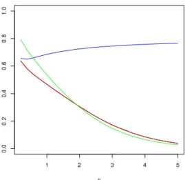
In Figure 1, the three approximations are compared to the exact value of P (M = 1|y) for a range of values of y. The correct simulation produces a graph that is indistinguishable from the true probability, while Congdon’s (2006) approximation stays within a reasonable range of the true value and Scott’s (2002) surprisingly drifts apart for most values of y.
◭ The correspondence of what is essentially Carlin and Chib’s (1995) scheme with the true nu-merical value of the posterior probabilities is obviously unsurprising in this toy example but more advanced setups see the approximation degenerate, since the simulations from the prior are most often inefficient, especially when the number of models under comparison is large. This is the reason why Carlin and Chib (1995) introduced pseudo-priors that were closer approximations to the true posteriors.
Acknowledgements
Both authors are grateful to Brad Carlin for helpful discussions and to Antonietta Mira for providing a perfect setting for this work during the ISBA-IMS “MCMC’ski 2” conference in Bormio, Italy. The second author is also grateful to Kerrie Mengersen for her invitation to “Spring Bayes 2007” in Coolangatta, Australia, that started our reassessment of those papers. This work had been supported by the Agence Nationale de la Recherche (ANR, 212, rue de Bercy 75012 Paris) through the 2006-2008 project Adap’MC.
References
Bartolucci, F., Scaccia, L., and Mira, A. (2006). Efficient Bayes factor estimation from the reversible jump output. Biometrika, 93:41–52.
Brooks, S., Giudici, P., and Roberts, G. (2003). Efficient construction of reversible jump Markov chain Monte Carlo proposal distributions (with discussion). J. Royal Statist. Soc. Series B, 65(1):3–55.
Carlin, B. and Chib, S. (1995). Bayesian model choice through Markov chain Monte Carlo. J. Roy. Statist. Soc. (Ser. B), 57(3):473–484.
Chen, C., Gerlach, R., and So, M. (2008). Bayesian model selection for heteroskedastic models. Advances in Econometrics, 23. To appear.
Chen, M., Shao, Q., and Ibrahim, J. (2000). Monte Carlo Methods in Bayesian Computation. Springer-Verlag, New York.
Chopin, N. and Robert, C. (2007). Contemplating evidence: properties, extensions of, and alterna-tives to nested sampling. Technical Report 2007-46, CEREMADE, Universit´e Paris Dauphine. Congdon, P. (2006). Bayesian model choice based on Monte Carlo estimates of posterior model
probabilities. Comput. Stat. Data Analysis, 50:346–357.
Congdon, P. (2007). Model weights for model choice and averaging. Statistical Methodology, 4(2):143–157.
Gelfand, A. and Dey, D. (1994). Bayesian model choice: asymptotics and exact calculations. J. Roy. Statist. Soc. (Ser. B), 56:501–514.
Gelman, A. and Meng, X. (1998). Simulating normalizing constants: From importance sampling to bridge sampling to path sampling. Statist. Science, 13:163–185.
Green, P. (1995). Reversible jump MCMC computation and Bayesian model determination.
Biometrika, 82(4):711–732.
Green, P. and O’Hagan, T. (1998). Model choice with mcmc on product spaces without using pseudo-priors. Technical report, University of Nottingham.
Newton, M. and Raftery, A. (1994). Approximate Bayesian inference by the weighted likelihood boostrap (with discussion). J. Royal Statist. Soc. Series B, 56:1–48.
Robert, C. (2001). The Bayesian Choice. Springer-Verlag, New York, second edition.
Scott, S. L. (2002). Bayesian methods for hidden Markov models: recursive computing in the 21st Century. J. American Statist. Assoc., 97:337–351.
Figure 1: Comparison of three approximations of P (M = 1|y) with the true value (in black): Scott’s (2002) approximation (in blue), Congdon’s (2006) approximation (in green), and correction
of Scott’s (2002) approximation (in red), indistinguishable from the true value (based on N = 106