HAL Id: hal-01168415
https://hal.archives-ouvertes.fr/hal-01168415
Submitted on 18 Sep 2018
HAL is a multi-disciplinary open access
archive for the deposit and dissemination of
sci-entific research documents, whether they are
pub-lished or not. The documents may come from
teaching and research institutions in France or
abroad, or from public or private research centers.
L’archive ouverte pluridisciplinaire HAL, est
destinée au dépôt et à la diffusion de documents
scientifiques de niveau recherche, publiés ou non,
émanant des établissements d’enseignement et de
recherche français ou étrangers, des laboratoires
publics ou privés.
transform keypoints: an approach combining fast
eigendecompostion, regularization, and diffusion on
graphs
Youssef Chahir, Bouziane Abderraouf, Mostefai Messaoud, Adnan Al Alwani
To cite this version:
Youssef Chahir, Bouziane Abderraouf, Mostefai Messaoud, Adnan Al Alwani. Weakly supervised
learning from scale invariant feature transform keypoints: an approach combining fast
eigendecom-postion, regularization, and diffusion on graphs. Journal of Electronic Imaging, SPIE and IS&T, 2014,
23 (1), pp.13. �10.1117/1.JEI.23.1.013009�. �hal-01168415�
Weakly supervised learning from scale invariant
feature transform keypoints: an approach combining
fast eigendecompostion, regularization, and
diffusion on graphs
Youssef Chahir,aAbderraouf Bouziane,a,b,*Messaoud Mostefai,band Adnan Al Alwania
aGREYC-UMR CNRS 6072 Campus II-BP 5186, Université de Caen 14032 Caen Cedex, France bUniversity of Bordj Bou Arreridj, MSE Laboratory, 34000, Algeria
Abstract. We propose a unified approach to propagate knowledge into a high-dimensional space from a small informative set, in this case, scale invariant feature transform (SIFT) features. Our contribution lies in three aspects. First, we propose a spectral graph embedding of the SIFT points for dimensionality reduction, which provides efficient keypoints transcription into a Euclidean manifold. We use iterative deflation to speed up the eigendecomposition of the underlying Laplacian matrix of the embedded graph. Then, we describe a variational framework for manifold denoising based on p-Laplacian to enhance keypoints classification, thereby lessening the negative impact of outliers onto our variational shape framework and achieving higher classification accuracy through agglomerative categorization. Finally, we describe our algorithm for multilabel diffusion on graph. Theoretical analysis of the algorithm is developed along with the corresponding connections with other methods. Tests have been conducted on a collection of images from the Berkeley database. Performance evaluation results show that our framework allows us to efficiently propagate the prior knowledge.
© 2014 SPIE and IS&T [DOI:10.1117/1.JEI.23.1.013009]
Keywords: high-dimensional data; graph-based learning; spectral graph embedding; regularization on graphs; classification; scale invariant feature transform features.
Paper 12218 received Jun. 7, 2012; revised manuscript received Oct. 27, 2013; accepted for publication Dec. 18, 2013; published online Jan. 21, 2014.
1 Introduction
Graph-based learning algorithms have spread in recent years, where initial information is asked to the user to highlight critical points of the considered space, subject to exploration. Consequently, the result is initialization dependent. How to avoid manual interactions with the user and efficiently propa-gate initial knowledge will be of a great interest in computer vision field and its related areas, where identification of objects in images is a challenging research subject. In this case, a family of segmentation algorithms have been devel-oped, where the image is modeled by a graph and the object to be extracted is one for which a certain form of energy functional is minimum.1,2 Different forms of energy
func-tional have been developed. In Ref. 3, the authors first use patches of different shapes and different sizes to extract different noise-robust features and then information theory-based measures are computed and minimized. In Ref.4, the energy functional to be optimized is defined using the geo-desic-distance combined with contours information, where the geodesic-distance region information is reevaluated according to the color model deduced by seeds introduced by the user.
On another plan, two main approaches can be distin-guished, whereas the segmentation process is either done automatically or guided by information provided by the user regarding the object of interest. To perform automatic segmentation, the authors in Ref. 5use the camera fixation
point on the object of interest to deduce a color model and a surrounding contour. Iterating this process minimizes the graph-cut energy and enhances the segmentation result. In a similar approach, the energy functional to minimize in Ref.6is expressed by an active contour model and the image is divided into two regions using a graph-cut. The object of interest is obtained by repeating this process until conver-gence to a defined threshold.
In the interactive approach, the user supplies initial seeds to differentiate between the object of interest and the back-ground, hence, avoiding object/background estimations, and depending on where the seeds are placed, two types of ini-tialization are studied: one relying on the definition of parts of the object and parts of the background,1,7and the other
one starts with an initial contour,8which may either enclose
the object, part of the object,9or delimit the border between
the object and the background.10However, this approach is
not effective if the segmentation process will be integrated into an automated framework. Moreover, the result is initial-ization dependent. Indeed, it is possible that, due to the com-plexity of the image, among the seeds introduced by the user to designate parts of the object (respectively, background), some of them are of the same class of the background (resp. object), or simply, the seeds are not representative enough. To avoid manual interactions, we investigate in this paper the use of the image keypoints as initial seeds to denote the ground truth. These are automatically extracted and they are first categorized and then diffused on the image to extract the
*Address all correspondence to: Abderraouf Bouziane, E-mail: bouziane
object of interest. A variety of keypoint descriptors have been proposed, such as Harris corner detector,11the scale invariant
feature transform (SIFT),12gradient location and orientation
histogram,13and difference of means.14The SIFT descriptors
are currently most widely used in computer vision applica-tions due to the fact that they are highly distinctive and invariant to scale, rotation, and illumination changes. In addi-tion, they are relatively easy to extract and to match against a large set of local features. Several improvements of SIFT features are proposed, including affine scale invariant feature transform (ASIFT)15and PCA-SIFT,16which applies
princi-pal components analysis to the SIFT descriptor in order to reduce the SIFT feature descriptor dimensionality from 128 to 36.
However, each keypoint is described by a considerable number of attributes and then distributed in a high-dimen-sional space. To overcome this constraint, in our approach we propose to construct a similarity graph over the SIFT descriptors. The eigendecomposition of the Laplacian matrix, associated to this graph, allows us to identify the dimensions that are carrying the relevant information. A Euclidean distance is then defined on these dimensions as proposed in Ref. 17, and the keypoints can be, therefore, classified through agglomerative categorization. However, if the image reveals a high number of keypoints, which is often the case, the size of the Laplacian matrix may slow down the calculation of eigenvalues and their correspondent eigenvectors and the segmentation algorithm, therefore, becomes very costly in computation.
Many works in the literature, including the matrix pertur-bation theory18,19 and the Nyström method,20,21 have been
proposed to accelerate the spectral decomposition via the approximation of the eigenvalues and their correspondent eigenvectors. In Ref. 22, the approximation to the leading eigenvector is based on a linear perturbation analysis of matrices that are nonsparse, nonnegative, and symmetric. Huang et al.23 studied the effects of data perturbation on
the performance of spectral clustering and its relation with the perturbation of the eigenvectors of the Laplacian matrix. In its turn, the Nyström method has been very successful. In Ref. 24, the authors show its use to approximate the eigendecomposition of the Gram matrix in order to speed up kernel machines. In Ref. 25, Fowlkes et al. present a technique for the approximate solution of spectral partition-ing for image and video segmentation based on the Nyström extension. Other variants of the Nyström method are pre-sented in Refs.26and 27
Practically, one can use the subjective scree-test of Cattell28
to determine the most important k’th dimensions that enclose the pertinent information. This criterion is based on the analy-sis of differences between consecutive eigenvalues, where a breakpoint would be located where there is the biggest change in the slope of the curve of eigenvalues. The first k’th eigen-values then correspond to the number of dimensions to retain (see Ref.29for detail). Another simple way is to consider the first dominant eigenvalues for which their sum is greater than a defined threshold (e.g.,≥80%).
1.1 Outline
The basic idea of our paper is to show how it is possible to learn from a restricted data set and propagate the acquired knowledge to a high-dimensional database. To evaluate
the effectiveness of our approach, in this article we focus on the case of image segmentation. The proposed framework operates in two phases. In the first phase, seeds are automati-cally identified and classified, and in the second phase, a propagation of these seeds on the graph allows to highlight the object of interest. The following steps outline our approach:
• A set of SIFT keypoints is extracted from the image and used to construct a visual similarity graph. A spec-tral embedding of this graph is performed to define a Euclidean reduced space.17To speed up the spectral
graph embedding, we propose to use the power itera-tion algorithm combined with the deflaitera-tion method to compute the first k’th largest eigenvalues and their corresponding eigenvectors, which are often well suited to define the new pose space basis. To help the categorization process, we perform a discrete regulari-zation of the graph constructed over the SIFT key-points expressed in their new coordinates. Thus, the clustering is done in the inferred regularized Euclidean manifold.
• At this step, a new graph is constructed over the image.
It will contain labeled vertices and unlabeled ones. By using our multilabel propagation algorithm, an energy functional is formulated and minimized. The objects of interest are then extracted when some conditions are satisfied.
It is worth mentioning that at each step, we will use a dif-ferent graph, i.e., a graph over the SIFT descriptors (feature space) to allow spectral embedding and a graph in the mea-sure space (the embedded space) to manifold regularization in order to enhance the accuracy of the keypoints categori-zation. Once the keypoints are labeled (classified), a final graph is constructed over the whole image (initial input data). It will contain labeled vertices and unlabeled ones. It will be used to propagate the information of the labeled keypoints in their neighborhoods. A graphical illustration of our framework is presented in Fig.1.
The rest of the paper is organized as follows. Section2
gives an overview of our spectral embedding framework. In Sec.3, we explain how to speed up eigendecomposition. In Sec.4, we present a discrete regularization on the graph in the embedded space to enhance data robustness. In Sec.5, a multilabel diffusion algorithm is detailed along with con-nections with other methods. Experimental results are pre-sented and commented in Sec. 6. In Sec. 7, we conclude our paper and discuss future extension.
2 Spectral Embedding Framework
The goal of the spectral analysis of the image to be seg-mented is to find an optimized pose space where relevant information is captured and similarity between pixels can be easily expressed. With this intention, a set of SIFT keys X ¼ fPt1; Pt2; : : : ; Ptng is extracted from an image through the local invariant feature extraction12(see Fig.2).
Each SIFT key Pti¼ ðXi; Ri; UiÞ is described by its two-dimensional location in the image Xi ¼ ðxi; yiÞ, its gradient magnitude and orientation Ri¼ ðri; aiÞ, and a descriptor vector Ui¼ ðui;1; : : : ; ui;128Þ, which represents the local tex-ture in the image. From the set X ¼ fPt1; Pt2; : : : ; Ptng ∈ Rl, we develop an appropriate Euclidean mapping
Y ¼ fy1; y2; : : : ; yng ∈ Rm representing the pose space (m≪ l). To do this, we build an undirected graph G on X and we learn a kernel matrix that respects the provided side-information as well as the local/nonlocal geometry of the SIFT features. Through the eigendecomposition of the matrix associated to the random walks on G, we define a diffusion distance Dðyi; yjÞ.
2.1 Random Walks on Graph
Let G ¼ ðV; E; wÞ be a weighted undirected graph, which is a finite set of vertices V ¼ fv1; v2; : : : ; vng connected by a finite set of edges E⊆V × V. Let fðvÞ be a function defined on the vertex v in a K-dimension space and represented by the tuple ff1; f2; : : : ; fKg ∈ RK. We denote by u∼ v the fact that the node u belongs to the ε-neighborhood of v [u∈ NεðvÞ], which is defined by NεðvÞ ¼ fu ∈ V; fðuÞ ¼ ðf0 1; · · · ; fK0Þ∕jfi− fi0j ≤εi; 0 < i≤Kg : (1) NεðvÞ includes all vertices close and similar to the vertex v. Also, we define a function F on the patch surrounding the vertex v as follows:
FðvÞ ¼ ffðuÞ; u ∈ NεðvÞg: (2)
For example, for a sequence of images, fðvÞ may be the spatiotemporal attributes of a vertex v. FðvÞ can represent the characteristics of the vertex in its neighborhood: a pattern projecting a composite element or a visual vocabulary.
We use a Gaussian kernel W to define the weight function and to give a measure of the similarity between a vertex and its neighbors. This weight function can incorporate local and nonlocal features and is defined by
wðu;vÞ ¼ 8 < : exp ! −kfðuÞ−fðvÞh2 k2 1 " · exp ! −kFðuÞ−FðvÞh2 k2 2 "
for each u∼v
0 otherwise
: (3) hi can be estimated using the standard deviation depending on the variations of jfðuÞ − fðvÞj and k FðuÞ − FðvÞk over the graph, respectively. So, given the scale parameter hi> 0, whiðu; vÞ → 0 when k :k ≫ hi and whiðu; vÞ → 1 when k :k ≪ hi.
We recall that the degree dðvÞ of a node v and the volume VolðGÞ of G are defined, respectively, by
dðvÞ ¼X
u∼vwðu; vÞ; and VolðGÞ ¼ X v∈VdðvÞ:
(4) The graph G reflects the knowledge of the local/nonlocal geometry of the data set X and is seen as a Markov chain; a random walk on this graph is the process that begins at some vertex u and at each time step, moves to another one v with a probability proportional to the weight of the corresponding edge. Thus, one can define the diffusion on G as the set of the possible visited vertices starting from a given one, where a transition is made in one time step from a vertex u toward another vertex v chosen randomly and uniformly among its neighborhood with the probability
pð1Þðu; vÞ ¼ PrðX
tþ1¼ vjXt¼ uÞ ¼wðu; vÞ
dðuÞ : (5)
The transition matrix P on G given by P ¼ fpð1Þðu; vÞju; v ∈ V; u ∼ vg explicits all possible one time step transitions and, therefore, provides the first-order infor-mation of the graph structure.
Let Pt be the t power of the matrix P, which denotes the set of all transition probabilities pðtÞðu; vÞ of going from one vertex u to another one v in t time steps. So, on the graph G, pðtÞðu; vÞ reflects all paths of length t between the vertex u and the vertex v. This t-time steps transition probability satisfies the Chapman–Kolmogorov equation that for any k such that 0 < k< t,
Fig. 1 Our diffusion framework.
50 100 150 200 250 300 50 100 150 200 250 300 350 400 450
pðtÞðu; vÞ ¼ PrðX
t ¼ vjX0 ¼ uÞ
¼X
y∈V
pðkÞðu; yÞ · pðt−kÞðy; vÞ: (6) It has been shown in Ref. 30that
lim
t→∞pðtÞðu; vÞ ¼ dðvÞ
VolðGÞ: (7)
2.2 Diffusion Maps-Based Clustering
For clustering purposes, a connection with the spectral decomposition of Pt is made (see Ref.31for detail) to gen-erate Euclidean coordinates for the low-dimensional repre-sentation of the vertices of the graph G at the time t, where, for each vertex, these coordinates are given by ΨtðuÞ ¼ ½λt1ψ1ðuÞ; λt2ψ2ðuÞ; : : : ; λtnψnðuÞ&T: (8) fλti; ψiðuÞg are the eigenvalues and the eigenvectors associ-ated with the normalized graph Laplacian of Pt. They cor-respond to the nonlinear embedding of the vertices of the graph G onto the new Euclidean pose space. Thus, the dif-fusion distance D2
tðu; vÞ between the nodes of the graph G can be expressed in the embedded space by
D2 tðu;vÞ ¼
X i≥1
λt2
i ½ψiðuÞ − ψiðvÞ&2¼ k ΨtðuÞ − ΨtðvÞk2: (9) We note, in particular, that this new distance depends on the time parameter t, which is considered here as a precision parameter, where, for large values, more information on the structure of the graph are captured. Based on their new coor-dinates, a classification of the SIFT keypoints can now be easily performed by using an agglomerative categorization algorithm based on the Euclidean distance defined in Eq. (9). 3 Eigendecomposition Speed Up
The eigenvalues of the matrix Ptare obtained by solving its characteristic equation
λnþ c
n−1λn−1þ cn−2λn−2þ : : : þ c0 ¼ 0: (10) But for large values of n, this equation is difficult and time-consuming to solve. An alternative method for approxi-mating these eigenvalues is to use the power iteration algorithm and the deflation method to find the dominant eigenvector and the corresponding eigenvalue, exploiting the fact that eigendecomposition of the matrix Pt provides a set of eigenvalues ordered as follows:
1¼ jλ0j ≥ jλ1j ≥ jλ2j ≥ : : : jλnj ≥ 0: (11) Indeed, the power iteration algorithm is a simple method for computing the largest eigenvector because it accesses to a matrix only through its multiplication by vectors. This prop-erty is particularly interesting in the case of large matrices. And the deflation method allows us to remove at each iter-ation the largest eigenvalue and rearrange the matrix so that the largest eigenvalue of the new matrix will be the second largest eigenvalue of the original matrix. This process can be repeated to compute the remaining eigenvalues.
3.1 Power Iteration Algorithm
To have a good approximation of the dominant eigenvector of the matrix Pt, one can choose an initial approximation V0, which must be a nonzero vector in Rnso that the sequence of its multiplication by Pt will converge to the leading eigen-vector. Algorithm1summarizes the power iteration method. In algorithm dividing by α in step 4 is to scale down each approximation before proceeding to the next iteration in order to avoid reaching vectors whose components are too large (or too small). For large powers, k, we will obtain a good approximation to the dominant eigenvector. Indeed, since Pt is a symmetric positive-semidefinite matrix, it has a basis of orthonormal eigenvectors fψig, and the initial approximation V0 can then be written as
V0¼X
n i¼1
βiψi; βi∈ R: (12)
Suppose that ψ1 is the eigenvector corresponding to the dominant eigenvalue λ1; then we can easily write
Vk¼ Pk tV0¼ Xn i¼1 βiPktψi¼ Xn i¼1 βiλkiψi ¼ β1λk1 # ψ1þ : : : þX n i¼2 βi β1 !λ i λ1 "k ψi $ : (13)
Since λ1 is the dominant eigenvalue, it follows that λi∕λ1< 1, and ∀ i > 1; lim k→ ∞ ðλi∕λ1Þk→ 0. We then deduce that Pk
tV0≈β1λk1ψ1, β1≠0, which means that the direction of Vkstabilizes to that of ψ
1, and since ψ1is a dominant eigenvector, it follows that any scalar multi-ple of ψ1is also a dominant eigenvector. Furthermore, since the eigenvalues of Ptare ordered like in Eq. (11), the power method will converge quickly if jλ1j∕jλ2j is small and slowly if jλ1j∕jλ2j is nearly equal to 1.
3.2 Deflation Method
Once an approximation to the dominant eigenvector ψi is computed, the Rayleigh quotient provides a correspondingly good approximation to the dominant eigenvalue λi, which is given by
Algorithm 1 The power iteration algorithm.
Require: V0, a nonzero vector in Rn
Ensure: An approximation to the dominant eigenvector 1: whilek Vk− Vk−1k ∕k Vkk ≥ ε do
2: Set Xk¼ PtVk−1
3: Set αk¼ the largest element of Xk(in absolute value)
4: Set Vk¼ Xk∕αk
5: end while
λi¼ðP t iψiÞT · ψi ψT iψi : (14)
To compute the remaining eigenvalues, one can modify the matrix Pt
i into Ptiþ1; : : : ; as follows: Pt iþ1¼ Pti− λi ψiψTi ψT iψi : (15) Pt
iþ1 has the same eigenvectors and eigenvalues as Pti except that λi is shifted to 0, leaving the other eigen-values unchanged. Indeed, for any eigenvector ψj, j ¼ ði þ 1; i þ 2; · · · ; nÞ of Pt, Pt iþ1 satisfies Pt iþ1ψj¼ Ptiψj− λiðψi ψT iÞ · ψj ψT iψi ¼ Ptψj− λi ψi · ðψTiψjÞ ψT iψi : (16)
Since the set of the eigenvectors fψig forms an orthonor-mal basis (i.e., ψT
iψj¼ 0), Ptiþ1ψj ¼ Ptiψj. Thus, the eigen-vectors of Pt
iþ1 are the same as those of Pti and its eigenvalues are λiþ1; · · · ; λn. The power method applied to Pt
iþ1will then pick out the next largest eigenvalue λiþ1. To determine the principal eigenvalues that gather the rel-evant information, the eigengap heuristic approach computes the gap between consecutive eigenvalues λkand λkþ1. The first λk carrying the principal information are those for which λk≫ λkþ1 (i.e., jλk− λkþ1j is relatively large). Practically, the 6∕7 first eigenvalues are sufficient to gather the pertinent information in the reduced space. To verify this method, we have conducted tests on different matrices of different sizes. We were limited to the 10th first important eigenvalues and eigenvectors. For example, in Fig. 3, the eigengap is well observed between the first and the second eigenvalue.
As shown in Fig. 4, there is practically no difference between the eigenvalues using this technique and those using the singular value decomposition (SVD) method.
However, regarding the computation time (see Fig. 5), it is clear that the iterative deflation approach is more efficient since it can compute only the first ones, while the SVD method has to decompose the whole matrix to extract the considered eigenvalues and eigenvectors and consequently consumes more time.
4 Manifold Regularization
Our motivation for this section is to transcribe the variational methods on a discrete graph. To this end, we propose to extend the scope of discrete regularization32to
high-dimen-sional data. We have implemented algorithms for regulariza-tion on graphs with p-Laplacian, p∈&0; þ∞½, for denoising and simplification of data in the embedded space. Readers can refer to Ref.33 for further details on this formalism.
Recall that the function f0is an observation of an original function f affected by noise n: f0¼ f þ n. The discrete
0 2 4 6 8 10 12 14 16 18 20 0 0.2 0.4 0.6 0.8 1 1.2 1.4 Lambda Values
The most important eigenvalues
Eigenvalues
Fig. 3 The most important eigenvalues.
0 100 200 300 400 500 600 700 800 900 1000 0 0.5 1 1.5 2 2.5 3 matrix size
the sum of the first 10th eigenvalues
Eigendecomposition using SVD and Iterative deflation
Iterative Deflation SVD
Iterative Deflation Error
Fig. 4 The sum of the first 10th eigenvalues using SVD and iterative deflation. 0 100 200 300 400 500 600 700 800 900 1000 0 1 2 3 4 5 6 7x 10 4 matrix size
computation time in milliseconds
The first 10th eigenvalues computation time using SVD and iterative deflation Iterative Deflation
SVD
Fig. 5 The first 10th eigenvalues computation time using singular value decomposition and iterative deflation.
regularization of f0∈ ðVÞ using the weighted p-Laplacian operator consists of seeking a function f'∈ ðVÞ, which is not only smooth enough on G, but also sufficiently close to f0. Variational models of regulation can be formalized by the minimization of two terms of energy using either the isotropic p-Laplacian or the anisotropic p-Laplacian. The isotropic model gives the following formulation of the min-imization problem: f' ¼ min f∈ ðVÞ # 1 p X v∈Vk ∇fvk p 2 þ λ 2k f − f 0k2 ðVÞ $ ; (17)
where p∈ 0; þ∞ is the smoothness degree and λ is the fidel-ity parameter, called the Lagrange multiplier, which specifies the trade-off between the two competing terms. ∇f repre-sents the weighted gradient of the function f over the graph. The solution of Eq. (17) leads to a family of nonlinear filters parametrized by the weight function, the degree of smooth-ness, and the fidelity parameter.
The first energy in Eq. (17) is the smoothness term or reg-ularizer, whereas the second is the fitting term. To solve the regularization problem, we use the Gauss-Jacobi iterative algorithm, where, for all ðu; vÞ in E:
8 > > > > < > > > > : fð0Þ ¼ f0 γðkÞðu; vÞ ¼ wðu; vÞðk ∇fðkÞðvÞkp−2 2 þ k ∇fðkÞðuÞk p−2 2 Þ fðkþ1ÞðvÞ ¼ pλf0ðvÞþP u∼v γðkÞðu;vÞfðkÞðuÞ pλþP u∼v γðkÞðu;vÞ ; (18) where γðkÞis the function γ at the step k. The weights wðu; vÞ are computed from f0 or can be given as an input.
At each iteration, the new value fðkþ1Þ at a vertex v depends on two quantities: the original value f0ðvÞ and a weighted average of the existing values in a neighborhood of v. We recall that the weighted gradient of the function f in a vertex v can be interpreted as the gradient magnitude at v. It may therefore be interpreted as the regularity of the function in the neighborhood of this vertex. It is defined as k ∇fðuÞk2¼ hX v∼uwðu; vÞðfv− fuÞ2 i1∕2 : (19)
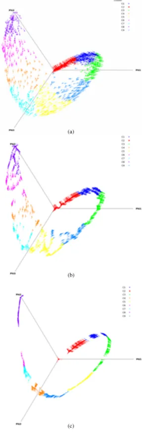
Figure6(a) represents the projection of SIFT keypoints cloud over its three principal components in the diffusion space. The graph is built in this space and the new coordi-nates are classified. As we can see, the parameter p consid-erably affects the result of the regularization. We observe the difference between Fig.6(b)with p ¼ 2 and Fig.6(c)with p ¼ 0.5. More simplification of the graph is obtained for p < 1. In this case, the manifold shape is more clear and the classification process is improved when p decreases. 5 Multilabel Diffusion Algorithm
5.1 Graph-Based Segmentation Method
Let V be the set of all image points, VL¼ fvkgmk¼1 be the set of labeled points (SIFT keypoints), and VU¼
fvugNu¼mþ1 be the set of unlabeled points. We extend the
function fðvÞ defined on the vertex v (see Sec. 2.1) to
incorporate its label value f0¼ l ∈ L ¼ f1; 2; : : : ; cg. So f will be represented by the tuple ff0; f1; : : : ; fKg. To make the similarity between the graph vertices insensitive to hi (see Sec.2.1), we normalize each wðu; vÞ as follows: wðu; vÞ ¼ wðu; vÞ∕½maxv∼uwðu; vÞ&.
According to the theory of graph-based semisupervised learning, the label propagation can be formulated as the
minimization of the energy function expressed in Eq. (17). Generally, we use p ¼ 2; then our strategy for propagating the labels can be formulated as an iterative process, where at every iteration step, only the labels of the unlabeled vertices are updated and the labels of the labeled ones will be clamped. For an unlabeled pixel v, its label at iteration t will be computed by 8 > > > < > > > : f ¼ ðf0; f1; · · · ; fKÞ f0 ¼ f 0 ∈ L ftþ1v ¼ 1 λþPu∼vwðu;vÞ h λf0 vþP u∼vwðu; vÞf t u i : (20)
If we set λ ¼ 0 and since pðu; vÞ ¼ wðu; vÞ∕ ½Pv∼uwðu; vÞ& [see Eqs. (4) and (5)], one can define the propagation process from a vertex u toward another vertex v by ftþ1 v ¼ 1 P u∼vwðu; vÞ X u∼vwðu; vÞf t u ¼ X u∼vpðu; vÞf t u:
Then, Eq. (20) can be rewritten as 8 < : f0 ¼ f 0 ∈ L ftþ1ðvÞ ¼P u∼vpðu; vÞf tðuÞ ∀ v ∈ V: (21)
Then, the multilabel propagation procedure on the graph G can be seen as a specific classification C on V and con-sidered as a function that assigns labels for each vertex v. f0ðvÞ ¼ argmax
l≤c Cvl: (22)
Initially, let C0
vl¼ 1 if v is labeled as l and C0vl¼ 0 other-wise. For unlabeled vertex v, C0
vl¼ 0.
Therefore, Eq. (22) can be reformulated as f0ðvÞ ¼ argmax
f0ðuÞ≤c
½f0ðvÞ ¼ f0ðuÞ&: (23)
The basic idea of our label propagation method is to con-sider an iterative algorithm where each node absorbs some label information from its neighborhood and updates its own label. This procedure will be repeated until all the nodes of the graph are labeled and not changed.
5.2 Links with Other Methods
Graph-based segmentation algorithms have been very suc-cessful in recent years. The modern variants are mainly built from a small set of basic algorithms: graph-cuts, random walk, and the shortest path algorithms. Recently, these three algorithms have been placed in a common frame-work that allows them to be considered as a special case of a general semisupervised segmentation algorithm with dif-ferent choices of parameters p and q.34
X ðu;vÞ∈E
½wðu; vÞpjfu− fvj&q; (24)
where wðu; vÞ is a function that measures the interactions between the nodes of the graph and jfu− fvj measures
the distance between them. Thus, our Eq. (21) can be easily driven from this framework if we pose p ¼ q ¼ 1 and pðu; vÞftðvÞ ¼ wðu; vÞjf
u− fvj. Furthermore, a connection between Eq. (21) and the energy minimization by Markov random field (MRF) models can also be established. Recall that an MRF is often described by a set of V vertices along with a neighborhood on them. On each vertex v, there is a random variable fðvÞ, which can take values from a finite set (e.g., fðvÞ ∈ L ¼ f1; 2; : : : ; cg). The goal is to find f' that satisfies f' ¼ argmin#X v ϕ½fðvÞ& þ X u∼v ϕuv½fðuÞ; fðvÞ& $ : (25)
ϕ½fðvÞ& is a function on the variable fðvÞ and can be defined as a likelihood energy where
ϕ½fðvÞ& ¼ 8 < :
∞ if ftþ1ðvÞ ≠ftðvÞ
ði:e:; the label ofv will be changedÞ 0 otherwise
; (26) and ϕuv½fðuÞ; fðvÞ& measures the information exchange between the labeled vertex u and the unlabeled vertex v. It can, in turn, be defined by referring to Eqs. (21) and (24) as ϕuv½fðuÞ; fðvÞ& ¼ pðu; vÞjfðuÞ − fðvÞj. pðu; vÞ is the probability corresponding to the random walk from u toward v. Since v has to be labeled, fðvÞ ¼ ∞; then the min-imization of Eq. (25) is equivalent to solving the following optimization problem:
min fðuÞ∈L
#X
u∼vpðu; vÞjfðuÞ − fðvÞj $
: (27)
Thus, we have shown that our method can be derived from the framework of energy minimization of MRF. 6 Experiments
We conducted our experiments on a collection of images issued from the Berkeley database.35 First, SIFT keypoints
are located on each image; then a visual similarity graph is constructed over these keypoints. Each vertex represents an SIFT keypoint and a weighed edge measures the similar-ity between two connected vertices u and v by using the Gaussian kernel wuv [Eq. (3)]. Fð:Þ is the histogram of the patch surrounding the considered point expressed in the LAB color space. Many variations of distances k Fu− Fvk2 can be used, including the Bhattacharya, Kolmogorov, inter-section, and correlation distances.36
Once the similarity between keypoints is defined, the eigendecomposition of the underlying Laplacian matrix leads to the definition of a new reduced pose space, where each SIFT keypoint is expressed by new Euclidean coordi-nates calculated according to its surrounding patch.
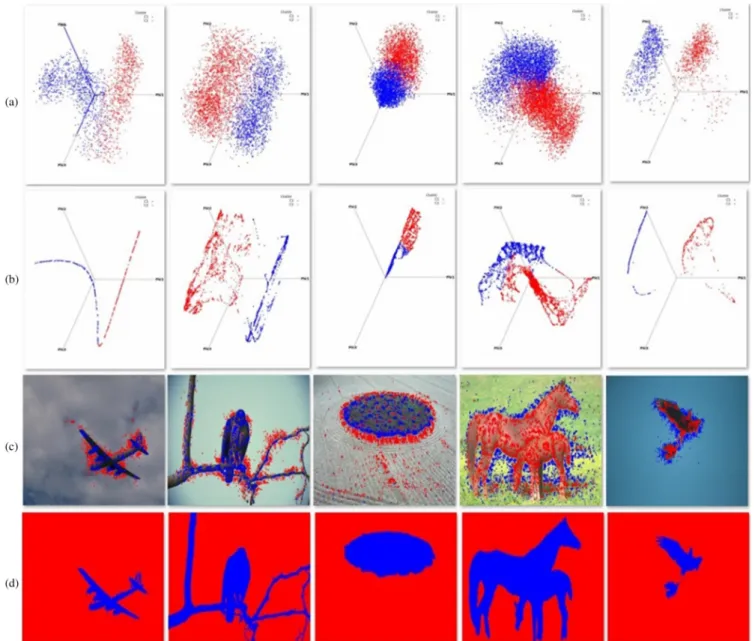
Figure 7 shows some classification results on the key-points cloud projected in the Euclidean pose space and their projections on the input images. The graphs in Fig. 7(b)
represent the regularized versions of those in Fig. 7(a)
with p ¼ 2. As we can see, this has highly made in evidence the object of interest class and the foreground class [see also Fig. 7(c)]. Figure 7(d) shows object/foreground
segmentation corresponding to the seeded images in Fig.7(c). These labels are propagated on the corresponding image graphs to extract the object of interest and obtained after 100 iterations using Eq. (21).
The F-measure, recall, and precision computed as described in Ref.37and corresponding to these images are shown in Table 1 (image1, image2, image3, image4, and image5 correspond to the images in Fig. 7(c)from left to right, respectively).
Figure 8 presents another example of multilabel image segmentation. In Fig. 8(a), SIFT keypoint classes are identified by using spectral embedding into a Euclidean manifold. These classes are better separated through mani-fold denoising with p ¼ 2 [Fig. 8(b)]. The projections of these classes on the images are presented in Figs. 8(c)
and 8(d).
To assess the performance of our framework, we used two objective segmentation measures: the Rand index (RI) and the global consistency error (GCE). The RI measures the consistency of a labeling between a given segmentation and
its corresponding ground truth by using the ratio of pairs of pixels having the same labels. The goal is to assign two pix-els to the same class if and only if they are similar in order to measure the percentage of similarity. The GCE measures the extent for which one segmentation can be viewed as a refine-ment of the other one. It is worth refine-mentioning that the sim-ilarity measure RI is better when it is higher and the distance measure GCE is better when it is lower. Often, GCE favors oversegmentation. Hence, to compare with other methods,
Fig. 7 Keypoints classification and their projections on the reduced space and the input images.
Table 1 F-measure, recall, and precision.
Image1 Image2 Image3 Image4 Image5 F-measure 0.8669 0.9211 0.9743 0.5937 0.9024 Recall 0.9911 0.9718 0.9734 0.4532 0.9996 Precision 0.7703 0.8754 0.9751 0.8606 0.8225
we have performed the segmentation without considering regions of an area <2% of the image.
A comparative evaluation of our method with four well-known ones, namely fuzzy C-means algorithm,38WaterShed
algorithm,39 normalized cuts,40 and the mean-shift
algo-rithm,41is implemented by using the library Pandore.42
We recall that the mean shift implementation performs clustering in a five-dimensional space with two spatial and three color dimensions. Note that the kernel width
has a very important effect on the algorithm performance. However, the choice of an appropriate value for the kernel width is still an open problem. In the present experiments, the spatial parameter hs is set to 10 and the range (color) kernel bandwidth was fixed to 20.
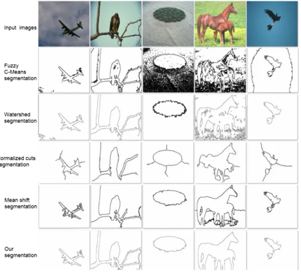
Figure 9 shows qualitative results of our algorithm applied on the same images in Fig. 7. It can be observed that when the seeds are well dispersed on the image, the seg-mentations have a closer similarity with the human one.
Quantitative results of our experiments are summarized by the histograms in Figs.10and11. These results clearly show that the original images and the results obtained by our approach are very close. Indeed, most of the GCE values found are <0.19, while a larger number of RI values are grouped below 0.8. The peaks found for GCE and for RI are 0.18 and 0.89, respectively. The corresponding seg-mented images are very similar visually and quantitatively. It can be seen from the x axis that the poor performance of segmentation from the GCE and the RI point of view are 0.01 and 0.53, respectively. This includes images that are difficult
to segment. This can be explained by the problem of borders and by the choice of segmentation parameters.
Table 2 presents the performance evaluation of our method compared with the state-of-art ones. As it can be observed, our method produces better results. It gives the lowest measure of GCE and the highest mean RI score.
The proposed method gives better results by producing a fewer number of homogeneous regions. Also, it provides a good solution to overcome the sensitiveness to the initial-ization condition of clusters. The oversegmentation is decreased effectively since this method integrates diffusion with automatic seeded region growing.
Fig. 9 The performance comparison with several segmentation approaches.
7 Conclusions
In this paper, we have addressed the problem of learning from a small informative set using a graph-based diffusion model. A case study was automatic image segmentation. We presented a unified framework through three steps: a spectral graph embedding of SIFT keypoints, manifold denoising with p-Laplacian, and a multilabel diffusion algo-rithm. With this scheme, a set of keypoints are automatically located on the image and, subsequently, distributed over the background and the regions of interest (ROIs). Thereafter, these seeds are propagated progressively on the graph, rep-resenting the image, which exploits the acquired semantic information and visual features among pixels until the seg-mentation of the ROI. We implemented the proposed frame-work and obtained encouraging experimental results. The proposed method produces good boundaries with respect to the ground-truth segmentation and relatively higher pre-cision compared with other methods. Nevertheless, the num-ber of classes needs to be specified in advance.
We currently explore the possibility of generalizing the concept of this framework for video segmentation by considering three-dimensional images representing the video keyframes and incorporating audio features to help our categorization.
Acknowledgments
This paper is supported by the PRETHERM ANR project No. ANR-09-BLAN-0352, co-financed by the French National Research Agency (ANR). The authors wish to thank the reviewers, the associate editor, and the editor-in-chief for their helpful suggestions and comments to improve this paper. We also would like the thank Professor Abder Elmoataz for discussions about the discrete p-regularization and its constructive remarks.
References
1. Y. Boykov and M. Jolly, “Interactive graph cuts for optimal boundary & region segmentation of objects in n-d images,” in Proc. 8th Intl. Conf. on Computer Vision, pp. 105–112, IEEE Computer Society (2001). 2. V. Kolmogorov and R. Zabih, “What energy functions can be
mini-mized via graph cuts,”IEEE Trans. Pattern Anal. Mach. Intell.26(2), 65–81 (2004).
3. G. Brunner et al., “Patch-cuts: a graph-based image segmentation method using patch features and spatial relations,” in Proc. of the British Machine Vision Conf., F. Labrosse, pp. 29.1–29.11, BMVA Press (2010).
4. B. L. Price, B. Morse, and S. Cohen, “Geodesic graph cut for interactive image segmentation,” in IEEE Conf. on Computer Vision and Pattern Recognition, pp. 3161–3168, IEEE Computer Society (2010). 5. N. D. F. Campbell et al., “Automatic 3D object segmentation in multiple
views using volumetric graph-cuts,”IVC J.28(1), 14–25 (2010). 6. J.-S. Kim and K.-S. Hong, “A new graph cut-based multiple active
contour algorithm without initial contours and seed points,”MVA J.
19(3), 181–193 (2008).
7. C. Rother, V. Kolmogorov, and A. Blake, “Grabcut: interactive fore-ground extraction using iterated graph cuts,” ACM Trans. Graph.
23(3), 309–314 (2004).
8. N. Xu, N. Ahuja, and R. Bansal, “Object segmentation using graph cuts based active contours,”Comput. Vis. Image Underst.107(3), 210–224 (2007).
9. A. Blake et al., “Interactive image segmentation using an adaptive GMMRF model,” in Proc. European Conf. in Computer Vision, pp. 428–441, Springer (2004).
10. J. Wang, M. Agrawala, and M. F. Cohen, “Soft scissors: an interactive tool for realtime high quality matting,”ACM Trans. Graph.26(3), 9 (2007).
11. C. Harris and M. Stephens, “A combined corner and edge detector,” in Proc. of the Alvey Vision Conf., C. J. Taylor, Ed., pp. 147–151, Alvety Vision Club (1988).
12. D. G. Lowe, “Distinctive image features from scale invariant key-points,”Int. J. Comput. Vis., 60(2), 91–110 (2004).
13. K. Mikolajczyk and C. Schmid, “A performance evaluation of local descriptors,”IEEE Trans. Pattern Anal. Mach. Intell.27(10), 1615– 1630 (2005).
14. H. Bay, T. Tuytelaars, and L. Van Gool, “SURF: speeded up robust features,”Int. J. Comput. Vis. Image Underst.110(3), 346–359 (2008). 15. J.-M. Morel and G. Yu, “ASIFT: a new framework for fully affine invariant image comparison,”SIAM J. Imaging Sci. 2(2), 438–469 (2009).
16. Y. Ke and R. Sukthankar, “PCA-sift: a more distinctive representation for local image descriptors,” in Proc. of the IEEE Computer Society Conf. on Computer Vision and Pattern Recognition, pp. 506–513, IEEE Computer Society (2004).
17. S. Lafon and A. B. Lee, “Diffusion maps, and coarse-graining: a unified framework for dimensionality reduction, graph partitioning, and data set parameterization,”IEEE Trans. Pattern Anal. Mach. Intell.28(9), 1393–1403 (2006).
18. G. W. Stewart and J.-g. Sun, Matrix Perturbation Theory, Academic Press, Boston (1990).
19. L. Ren-Cang, “On perturbations of matrix pencils with real spectra, a revisit,”Math. Comput.72(242), 715–728 (2003).
20. E. J. Nyström, “Über die praktische Auflösung von Integralgleichungen mit Anwendungen auf Randwertaufgaben,”Acta Mathematica54(1), 185–204 (1930).
21. C. T. H. Baker, The Numerical Treatment of Integral Equations, Clarendon Press, Oxford (1977).
22. A. Robles-Kelly, S. Sarkar, and E. R. Hancock, “A fast leading eigen-vector approximation for segmentation and grouping,” in Proc. 16th Int. Conf. on Pattern Recognition, pp. 639–642, IEEE Computer Society (2002).
23. L. Huang et al., “Spectral clustering with perturbed data,” in Advances in Neural Information Processing Systems, pp. 705–712, Curran Associates, Inc. (2008).
24. C. Williams and M. Seeger, “Using the Nyström method to speed up kernel machines, in Advances in Neural Information Processing Systems, pp. 682–688, MIT Press (2001).
25. C. Fowlkes et al., “Spectral grouping using the Nyström method,”IEEE Trans. Pattern Anal. Mach. Intell.26(2), 214–225 (2004).
26. J. C. Platt, “FastMap, MetricMap, and Landmark MDS are all Nyström algorithms,” in 10th Int. Workshop on Artificial Intelligence and Statistics, pp. 261–268 (2005).
27. K. Zhang and J. T. Kwok, “Density-weighted Nystrom method for computing large kernel eigensystems,”Neural Comput.21(1), 121–146 (2009).
28. R. B. Cattell, “The scree test for the number of factors,”Multivariate Behav. Res.1(2), 245–276 (1966).
29. G. Raiche, M. Riopel, and J. G. Blais, “Non graphical solutions for the Cattell’s scree test,” in Proc. Int. Annual Meeting of the Psychometric Society, Montreal, Canada (2006).
30. S. Lafon, Y. Keller, and R. R. Coifman, “Data fusion and multicue data matching by diffusion maps,”IEEE Trans. Pattern Anal. Mach. Intell.
28(11), 1784–1797 (2006).
31. B. Nadler et al., “Diffusion maps—a probabilistic interpretation for spectral embedding and clustering algorithms,” in Principal Manifolds for Data Visualization and Dimension Reduction, A. N. Gorban et al., Eds., Vol. 58, pp. 238–260, Springer, Berlin, Heidelberg (2007). 32. M. Ghoniem, Y. Chahir, and A. Elmoataz, “Nonlocal video denoising,
simplification and inpainting using discrete regularization on graphs,”
J. Signal Process.90(8), 2445–2455 (2010).
33. A. Elmoataz, O. Lezoray, and S. Bougleux, “Nonlocal discrete regulari-zation on weighted graphs: a framework for image and manifold processing,”IEEE Trans. Image Process.17(7), 1047–1060 (2008). Table 2 Performance evaluation of our algorithm.
Global consistency error Rand index Ground truth (human) 0.079 0.875 Fuzzy C-means 0.221 0.789 Watershed 0.203 0.697 Normalized cuts 0.218 0,723 Mean-shift 0.259 0.755 Our approach 0.189 0.799 Note: Bold values show the results obtained by our approach.
34. A. Sinop and L. Grady, “A seeded image segmentation framework uni-fying graph cuts and random walker which yields a new algorithm,” in IEEE 11th Int. Conf. on Computer Vision, pp. 1–8, IEEE Computer Society (2007).
35. D. Martin et al., “A database of human segmented natural images and its application to evaluating segmentation algorithms and measuring ecological statistics,” in Proc. 8th Int’l Conf. on Computer Vision, Vol. 2, pp. 416–423, IEEE Computer Society (2001).
36. L. Ballan et al., “Video event classification using string kernels,”
Multimed. Tools Appl.48(1), 69–87 (2010).
37. M. Kulkarni and F. Nicolls, “Interactive image segmentation using graph cuts,” in Twentieth Annual Symp. of the Pattern Recognition Association of South Africa, pp. 99–104 (2009).
38. J. C. Bezdek, R. Ehrlich, and W. Full, “FCM: the fuzzy c-means clustering algorithm,”J. Comput. Geosci.10(2–3), 191–203 (1984). 39. L. Vincent and P. Soille, “Watersheds in digital spaces: an efficient
algo-rithm based on immersion simulations,”IEEE Trans. Pattern Anal. Mach. Intell.13(6), 583–598 (1991).
40. J. Shi and J. Malik, “Normalized cuts and image segmentation,”IEEE Trans. Pattern Anal. Mach. Intell.22(8), 888–905 (2000).
41. D. Comaniciu and P. Meer, “Mean shift: a robust approach toward feature space analysis,”IEEE Trans. Pattern Anal. Mach. Intell.24(5), 603–619 (2002).
42. “Pandore: Une bibliothèque d'opérateurs de traitement d'images,” Version 6.6,https://clouard.users.greyc.fr/Pandore(2013).
Youssef Chahir is a professor in the computer science department at Lower Normandy University. He is a member of the Image Team at the GREYC Laboratory. His research interest fields include image and video processing and analysis, multimedia data mining, spectral analysis and restitution, and animation in virtual environments. Abderraouf Bouziane is an associate professor at the computer sci-ence department at Bordj Bou Arreridj University. He is a member of the MSE Laboratory. He worked as an invited researcher at GREYC Laboratory. His research interest fields include spectral analysis, organization, and indexing of high-dimensional multimedia data. Messaoud Mostefai is an associate professor at the computer sci-ence department at Bordj Bou Arreridj University. He is a member of the MSE Laboratory. His main research interests are focused on classification and biometric identification, computer vision and signal processing.
Adnan Al Alwani is a PhD student at the Image Team, Lower Normandy University. His research interest fields include pattern rec-ognition, signal, image, and video processing.