Condition-based maintenance applied to rail freight car components : the case of rail car trucks

Condition-Based Maintenance Applied to Rail Freight Car Components

---

The Case of Rail Car Trucks

by Qian Ma

B.E., Jilin University of Technology, China (1990) M.S., University of North Florida (1995)

Submitted to the Department of Civil and Environmental Engineering in Partial Fulfillment of the Requirements

for the Degree of

Master of Science in Transportation at the

Massachusetts Institute of Technology May 1997

© 1997 Massachusetts Institute of Technology All rights reserved

Signature of Author... .. . a....:.... ...

Department of Civil and Environmental Engineering May 1997

Certified by ... ... ... ... ...

Carl D. Martland Senior Research Associate, Department of Civil and Environmental Engineering Thesis Supervisor

Accepted by ... ... ...

Joseph M. Sussman Chairman, Departmental Committee on Graduate Studies Department of Civil and Environmental Engineering

OF TrC'. .

Condition-Based Maintenance Applied to Rail Freight Car Components

--- The Case of Rail Car Trucks

by Qian Ma

Submitted to the Department of Civil and Environmental Engineering in Partial Fulfillment of the Requirements

for the Degree of

Master of Science in Transportation

ABSTRACT

Maintenance of the various components of rail freight car continues to be an extremely important concern to railroad decision makers. Varied policies for rail freight car maintenance not only have an impact on rail car availability but also effect the operating cost, freight damage rate and safety.

In this research, condition based maintenance (CBM) policy is proposed for the maintenance of rail freight car components, especially freight car trucks, in order to obtain the greatest benefits from maintenance activity in the system level. In order to capture all the system level consequences of a given maintenance policy, an economic model based on life cycle cost is used.

Model results show that CBM can save 5% to 12% of life cycle cost relative to two alternative maintenance policies, even when the inspections are not perfect (i.e., a 70-80% correct prediction rate). The sensitivity analysis indicates that the result is quite robust.

This research also addresses the issue of when to use premium trucks and when to use standard trucks. Even though premium trucks are more expensive than standard truck, they have better performance, and longer life. If a freight car is highly utilized, premium trucks have about 5% lower life cycle cost comparing to standard trucks under the preferred CBM maintenance policy.

Thesis Supervisor: Carl D. Martland.

ACKNOWLEDGEMENTS

First I would like to thank my thesis advisor, Mr. Carl D. Martland. The many long discussions I had with him were not only essential to the completion of this thesis but will benefit the rest of my life.

Dr. Patrick Little, my former research advisor, led me into the interesting field of freight car maintenance. His advice was always helpful and insightful.

Conrail Hollidaysburg Car Shop Manager, Mr. Dennis L. Beecher and his staff were very kind to assist me to conduct a week long field studies.

Many thanks to my wonderful M.I.T Rail group and CTS fellows. Hong Jin and Bill Robert were always there whenever I need help on whatever matter. The group

studies on number of courses with Xing Yong, and Alex Reichert and Julie Wei were very helpful. I had a wonderful time with CTS soccer team, thanks to Joe Barr, Owen Chen, Scott Ramming, Constantinos Antoniou, Paul Carlson, ... Many other name should mentioned here, John Trever, Lisa Klein, Yi yi He, Sam Lau,, Suzy Wang, Yan Dong, Jeff Chapman, Abel Munoz Loustaunau, Stanley Ouyang ...

I also would like to acknowledge the Center for Transportation Studies at MIT and the Association of American Railroad for financially support my entire research and study at MIT.

Contents

List of Figure ... ... 6

List of Tables ... 7

Chapter 1. Introduction ... 8

1.1. Problem Statem ent... ... 8...

1.2. Research Contributions ... 10

1.3. Structure of the Thesis ... 11

Chapter 2. Basic Concepts of Maintenance ... 12

2. 1. Definition of Maintenance ... 13

2.2. Alternative Maintenance Policies ... ... 17

2.3. Condition Based Maintenance ... ... ... 17

2.3.1. The accuracy of Inspection ... 17

2.3.2. Literature Review On Inspection Interval... 19

2.3.3. Literature Review On Applications of CBM ... 25

Chapter 3. Inspection Approach to Support the Application of CBM...30

3.1. Three -Piece Freight Car Truck and Inspection ... 30

3.1.1. O verview ... 30

3.1.2. External Condition and Inspection...38

3.1.3. Internal Condition and Inspection...41

3.2. Inspection Approaches to Support CBM ... .... 45

3.2.1. Review of Statistical Forecasting Techniques ... 45

3.2.1.1. Discrete Choice Method ... ... 46

3.2.1.2. Performance Threshold Method...52

3.2.2. Previous Data Modeling ... 55

3.2.3. Continuous Data Modeling ... 56

Chapter 4. 4.1. 4.2. 4.3. 4.4. 4.5. 4.6. 4.7. 4.8. An Economic Model of CBM ... .. ... 61 Introduction ... ... 61

Description of Components for Life Cycle Cost...64

Operating Cost Model... ... 65

Truck Life Model for Periodic Replacement Policy... 69

Inspection Interval Model ... ... ... 71

Life Cycle Cost Under Imperfect Inspection ... 75

Sensitivity Analysis...81

Integrated Model and Results ... 83

Chapter 5. A Policy Analysis: Premium Truck vs. Standard Truck ... 87

5.1. Introduction... ... 87

5.3. CBM applied to Premium Truck... 89

5.4. Premium Truck and Standard Truck under Alternative Maintenance Policies ... 92

Chapter 6. Summary, Conclusion and Future Research ... 95

6.1. Summary of the thesis... ... 95

6.2. C onclusion ... ... 97

6.3. Future Research... ... 98

List of Figures

1.1. The Structure of The Thesis ... 11

2.1. Periodic Replacement Policy ... ... ... 16

2.2. CBM Procedure ... 29

3.1. Train-Track System... 31

3.2. Three-piece Freight Car Truck... ... 33

3.3. Truck Side Frame...34

3.4. Truck Bolster ... 35

3.5. Truck Suspension System ... 36

3.6. Wear Surfaces and Liners around Friction Shoe...37

3.7. Bolster Center Plate ... 44

4.1. Maintenance Policy and Life Cycle Cost... ... ... 62

4.2. Freight Car Truck Operating Cost Curve... 67

4.3. Cut-Off Limit for Periodic Replacement Policy and Rail Car Truck Life Distribution... 71

4.4. Freight Car Truck Deterioration Curve...72

4.5. Inspection Interval Determination... ... 74

4.6. Percentage of Replacement Under Different Condition Stage for Condition Limit 0.4 ... 79

List of Tables

2.1. Sensitivity and Specificity... ... 18

3.1. External M easurem ent... ... 57

3.2. Calculation of Sensitivity and Specificity for First Round M odel ... ... ... ... 60

4.1. Life Cycle Cost Components for Standard Truck ... .... 65

4.2. Freight Car Truck Life and Operating Cost (Standard Truck)...68

4.3. Cumulative Failure Rate and Life for Standard Truck... 70

4.4. CBM: Optimal Condition Limit and Inspection Interval Under Perfect Inspection... ... 75

4.5. Real Condition Vs. Perceived Condition ... 77

4.6. CBM: Life Cycle Cost Under Imperfect Inspection (Standard Truck) ... ... 80

4.7. Real Condition Distribution Assumptions ... ... 82

4.8. Sensitivity Analysis for Imperfect Inspection...83

4.9. Life Cycle Cost of Freight Car Truck Based on Three Maintenance Policies ... ... ... 84

5.1. Comparison on Cost Components between Standard and Premium Truck ... ... 88

5.2. CBM: Optimal Condition Limit and Inspection Interval for Premium Truck Under Perfect Inspection...90

5.3. CBM: Life Cycle Cost Under Imperfect Inspection (Prem ium Truck)... ... 91

Chapter 1

INTRODUCTION

1.1. Problem Statement

Maintenance of the various components of rail freight car continues to be an extremely important concern to railroad decision makers. Freight cars are an important and integral part of the rail transportation system. Varied policies for rail freight car maintenance not only have impact on car availability but also effect operating cost, freight damage rate and safety. The most commonly used policies in practice are to replace upon failure or to replace periodically. Problems associated with replacement upon failure are that it would result in a higher operating cost, incur failure cost and also raise safety concerns. For the periodic replacement policy, it is hard to decide the right life limit at which components will be replaced. The same components on different cars may have different lengths of physical lives because of different usage patterns. If the replacement limit is conservative, a risk exists that the component may be replaced under the scheduled maintenance regime well before its useful life has elapsed; this would result in excessive and unnecessary maintenance and higher life cycle costs. In the cases where the replacement limit is too optimistic, many components will fail before being replaced, and costs will be similar to replace upon failure.

In this research, condition based maintenance (CBM) policy is proposed for freight car components in order to obtain the greatest benefits from system maintenance. CBM is the strategy by which maintenance is undertaken only when the component or system reaches a particular state or condition, usually one which is believed to be a

precursor to in-service failure. CBM allows railroads to replace a component after it has had a fairly long life, but before it deteriorates so much as to cause sharply increased operating cost or a significant risk in-service failure. CBM therefore is like to result in the lowest life cycle cost among the three policies.

In this thesis, the maintenance of freight car components is our general concern while maintenance of freight car truck is studied in detail because freight car trucks present a useful example of many of the problems associated with developing and implementing an effective CBM program. At the heart of CBM is the ability to measure or estimate the true condition of the component, and to determine what action to take in response. The freight car truck is the lower part of freight car, which acts as an interface between the car body and the rail track and enables the movement of the cars. In order to apply CBM to freight car trucks, the true internal conditions have to be known or detected which is a difficult because the internal parts are located under the car bodies and cannot be observed directly without lifting the car bodies off the truck.

In order to capture all the consequence of a given maintenance policy in the system level, life cycle cost is used. Life cycle cost is the sum of initial cost, operating costs, inspection cost, replacement cost and failure cost, divided by life of the component. The reason that operating cost is being included is because different maintenance policies would result in different conditions for freight car trucks over time, and different truck conditions have different effects on the operating costs.

An economic model is developed in order to compare the impacts on life cycle cost under those three maintenance policies and to illustrate how CBM can be

issue of when to use premium truck and when to use standard truck. Generally speaking, premium trucks have higher initial cost but better performance than standard trucks do. For new cars and for replacement of trucks on old cars, a question raised in practice is which kind of truck is more economical. This would be influenced by the type of commodities the cars carry, the usage pattern of the cars, the current condition of other part of car components, and other factors.

1.2. Research Contributions

This research makes three contributions to the state of knowledge about

transportation systems and vehicle maintenance. First, it systematically evaluates various maintenance policies being used in rail freight car truck maintenance. It does this by analyzing the advantages and disadvantages associated with each maintenance policy and then demonstrating this in a economic model of freight car trucks.

The second contribution is that a framework of applying CBM to rail freight car components is developed. In the case of freight car truck, it shows that CBM would result in the lowest life cycle cost among three policies.

The third contribution is that the issue of when to use premium truck and standard truck is addressed by employing the economic model of freight car truck. This provides fresh insight from a system point of view.

1.3. Structure of the Thesis

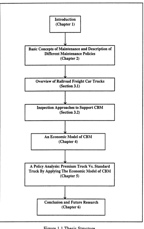
This thesis is organized along the line of general discussion of maintenance theories, modeling and application, and is illustrated in the flow chart in Figure 1.1.

Introduction (Chapter 1)

Basic Concepts of Maintenance and Description of Different Maintenance Policies

(Chapter 2)

Overview of Railroad Freight Car Trucks (Section 3.1)

Inspection Approaches to Support CBM (Section 3.2)

An Economic Model of CBM (Chapter 4)

A Policy Analysis: Premium Truck Vs. Standard Truck By Applying The Economic Model of CBM

(Chapter 5)

Figure 1.1 Thesis Structure

Conclusion and Future Research (Chapter 6)

Chapter 2

Review of Maintenance Policies

This chapter first reviews the basic concepts of maintenance and analyzes the advantages and disadvantages of common maintenance policies. It then describes some key issues of applying CBM, i.e., sensitivity and specificity of inspection techniques. Finally, it summarizes some applications of CBM in non-rail industries to give some insights on applying CBM to rail car components.

2.1. Definition of Maintenance

Maintenance is a combination of any actions carried out to retain an item in, or restore it to, an acceptable condition in a cost effective manner [Williams et al., 1994].

The key phrases are "an acceptable condition" and "in a cost effective manner". In the case of the maintenance of rail freight car trucks, the condition of trucks not only affects the quality of service railroads provide, but also affects the overall operating cost (as will become clear in later chapters). An acceptable condition for rail freight car trucks therefore implies a state of truck in which the system provides a safe and reliable service with a low operating cost. This shows that when considering a maintenance program or policy for rail freight car trucks, railroads must take account of both the performance of a truck in terms of service and the impact it has on operating cost.

If railroads have little concern on other factors, they can maintain rail freight car trucks in good condition by frequently replacing them with new trucks. However, this will result in a low utilization of the components and more down time for the freight cars.

In order to take above concerns into account, life cycle cost must be used. Life cycle cost is the sum of initial cost, operating cost, inspection cost and maintenance cost, divided by life of the component. It can be calculated as follows,

init cost + op_ cost + insp_ cost + instal cost + fail cost

LCC =

life

(2.1)

where LCC is the life cycle cost for a component; init_cost is the cost used to purchase the component when it was new; op_cost is the additional operating cost due to the component, this may become more clear when explained in chapter 4; insp_cost is the cost associated with inspection for some maintenance policy; instal_cost is the cost associated with the repair/replacement of the component; fail_cost is the cost caused by the failure of the component.

Generally speaking, a maintenance policy which results in a longer life and lower cost in one or more above cost components is preferred.

2.2. Alternative Maintenance Policies

In this section, we describe two common maintenance policies, i.e., periodic replacement and replace upon failure. We then analyze the advantages and disadvantages associated with these policies.

Replace upon failure is a policy that can be characterized as "do nothing until it breaks". This policy allows the components maintained to have the maximum life span. The problem associated with it is that it would result in a higher operating cost, failure

cost and, for some components, may cause of safety concerns. This policy is applied to number of low cost or non-critical components, such as tie.

This is generally only a reasonable strategy when the true condition is not knowable, the components is not subject to an increasing failure rate, or the costs of failure are low relative to the costs of replacing unfailed components. If the components fail randomly and provide no prior indication of impending failure, this type of

maintenance remains the only option. Even if the condition of component can be obtained, but only through a costly inspection method, and the costs of failure are lower than the cost of inspection, then this replace upon failure strategy is still justified. Another case involves production processes with certain time cycle or season feature. For

example, some manufacturing systems work in weekly basis, 5 days production, two weekend days off; or in daily basis, works from 8:00 AM to 5:00 PM. If the cost of failure for some component is low and replacing the unfailed components will interrupt the normal production, it may be better off to perform the maintenance activity in off production period.

Periodic maintenance is a policy that system components are replaced in a

predetermined interval. In an ideal situation, the predetermined interval is an optimal one for some components in every rail freight car so that the service reliability is high and

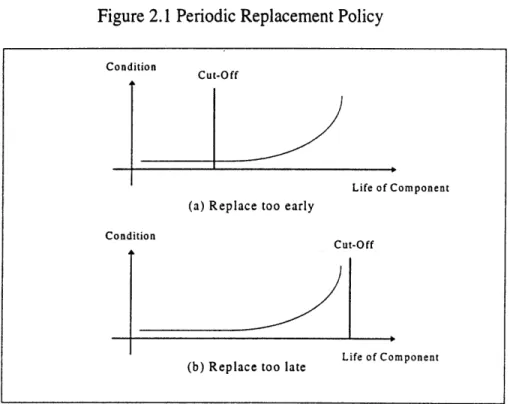
operating cost is low. However, in reality, this optimal interval is hard to obtain. Even for the same components, they may have different physical lives because of different usage patterns. Figure 2.1 shows the two extreme cases. If the replacement limit is conservative, a risk exists that the component may be replaced under the scheduled maintenance regime well before its useful life has elapsed (figure 2.1(a)). This result in the conduct of

excessive and unnecessary maintenance and subsequent costs. In the cases where the replacement limit is too optimistic and the components fail before being replaced (figure 2.1(b)), costs similar to replacement upon failure will occur.

Figure 2.1 Periodic Replacement Policy

(a) Replace too early Condition

C

(b) Replace too late

LCe o1 Component :ut-Off Life of Component Condition Cut-Off I ~^I---.

2.3. Condition Based Maintenance

Condition-based maintenance (CBM) is the strategy by which maintenance is undertaken only when the component or system reaches a particular state or condition, usually one which is believed to be a precursor to in-service failure. Because CBM allows railroads to replace a component of a rail car at the right point where it has had a fairly long life and where continued use would cause sharply increased operating cost and further might cause in-service failure, CBM would result in the lowest life cycle cost among three policies.

The definition of CBM implies there are three critical issues for CBM to be successful. The first critical issue is the accuracy of the inspection. CBM requires that there is some means of determining the true condition of the component, this is usually done by inspection. The accuracy of the inspection will directly affect the result of CBM.

The second critical issue is the inspection interval. Every inspection has a cost associated with it. This normally includes the labor cost involved in inspection; some times there is a cost for out off service time if the normal production has to be interrupted for inspection. If the inspection interval is short, the number of total inspections will be high. The inspection cost will be high also. On the other hand, if the inspection interval is not short enough to catch the defect, the component will fail, and there are costs

associated with component failure.

The last critical issue is the condition limit. The condition limit has affects on the life of the component and the operating cost of the system. Here the condition refers to wear, good components have low wear and bad components have high wear. If the condition limit is set very low, then components will have a shorter life. On the other

hand, if condition limit is set very high, the operating cost will become very high because the condition of component has deteriorated to a level where the system cannot function as it should.

In this section, first, the accuracy of inspection is discussed. Second, some literature on inspection intervals is reviewed. Finally some of the CBM applications are reviewed.

2.3.1. The accuracy of Inspection

In general, when a component is inspected, the true condition of maintained asset may not be obtained with 100 percent accuracy due to varied reasons. Therefore we need some indicators to measure the accuracy of inspection. One obvious indicator is the correctly predicted rate, which is the percentage of the samples that their believed conditions from inspection match their true conditions. However, this indicator is not effective enough to tell the whole story.

Suppose there are 100 samples, of which 90 are in good condition and 10 are in bad condition. However, the inspection results are different: we believe that all 90

samples which are actually in good condition are in good condition, but only 5 of the 10 samples which are actually in bad condition were found to be bad. The overall correctly predicted rate is 95 percent, which is quite good, but we missed half of the bad samples. In medical examination and inspection literature, sensitivity and specificity are often used to describe the accuracy of an inspection method [Muller et al., 1990]. "Positive" and "negative" are the terms used to described the test result of a medical examination. If a test for a disease is positive, it means the disease is not present. If the

test is negative, the disease is present. Sensitivity can be used to describe the ability of an examination to detect the disease if the disease is present indeed. Specificity is the ability to detect healthy people if the people are really healthy. In other words, sensitivity

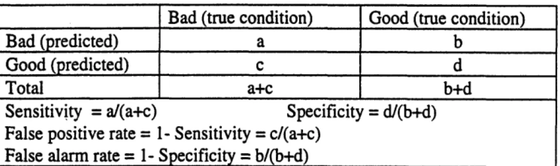
(specificity) tells the probability that an examination finds a person with (without) the disease, given that the person really does (does not) have the disease. False positive rate is the underestimation rate of an examination, and false alarm rate is the overestimation rate of an examination. Here sensitivity and specificity can be helpful to measure the overall effectiveness of an inspection along with the false negative rate and the false alarm rate. They can be calculated by using formulas in table 2.1.

Table 2.1 Sensitivity and Specificity

Bad (true condition) Good (true condition)

Bad (predicted) a b

Good (predicted) c d

Total a+c b+d

Sensitivity = a/(a+c) Specificity = d/(b+d) False positive rate = 1- Sensitivity = c/(a+c)

False alarm rate = 1- Specificity = b/(b+d)

In the example above, we had 100 samples, 90/10 split for good and bad conditions. For the 90 samples in good condition, the perceived conditions from

inspection were all good. For the 10 samples in bad conditions, the perceived conditions from inspection were 5 good and 5 bad. Then the specificity for this inspection method is 90/90 = 100% and false alarm rate is 100-100 = 0% while the sensitivity is 5/10 = 50% and false positive rate is also 50%.

2.3.2. Literature Review On Inspection Interval

The examinations scheduling problem or inspection interval problem have long been the subject of research in the medical screening field. One of the most effective ways to control a chronic disease is screening -examining seemingly healthy individuals to detect the disease before the surfacing of clinical symptoms and enable early and more effective treatment [Morrrison, 1985]. If it is established that a particular screening procedure is medically desirable, there remains the practical necessary of determining whether of not the costs involved would be worthwhile [Shahani and Crease, 1977]. Clearly in these days of scarce resources it is necessary to search for screening policies that will make the procedures as efficient as possible. Many variables influence the efficiency of a screening program, and inspection interval is one of the most important variables.

Following are reviews of the research on this topic. The reviews will focus more on the methodology, especially on how the problem is structured and formulated, rather than how the solution is derived mathematically. The mathematical solution is important to implement the system, but it varies with the nature of problem. On the other hand, the methodology may be applicable to different applications with justification.

(1) Optimum Checking Procedures (1963) by Barlow, Hunter and Proschan One of the classical and probably one of the most important work on this topic is done by Barlow et al [1963]. In that research, it states that the problem of checking or inspection often arises in connection with systems that are deteriorating. It assumes that deterioration is stochastic and that the condition of the system is known only if it is inspected. It further assumes that upon detection of failure, the problem ends. The

optimization problem considered here is to minimize the total expected value of the cost of the lapsed time between system failure and its detection and the cost of checking.

As an example consider the problem of detecting some grave physical illness such as cancer by successive medical examinations. Each examination costs money and takes time so we do not wish to examine too often. On the other hand, the longer the time elapsed between occurrence and detection of the condition, the greater the "cost".

Therefore, two costs are considered : (1) each check entails a fixed cost c,; (2) the time elapsed between system failure and its discovery at the next check results in a cost c2 per unit of time. Let N(t) denote the number of checks in [0,t] and r, the time to discovery if the system fails at time t. Then the loss is

c,

[N(t)

+

1]

+

c

r

,

(2.2)

for a given system with failure distribution F, the expected loss is

E(loss) =

fc,

{[M(t)

+1]+

cE[r;]

}dF(t),

(2.3)

where M(t) = E[N(t)].

Any checking procedure that minimizes this objective function is called an optimum checking procedure.

To specify a checking procedure it is sufficient to specify a sequence of random variables { Yk}, _{called the inter-checking times, or inspection interval. If the random}

variables are identically distributed, the associated checking procedure is called periodic. If the random variables are not identically distributed, the checking procedure is called

sequential. Barlow et al. concluded that periodic checking procedures are optimum over the class of sequential checking procedures only for systems which fail according to an exponential distribution. In this case, the optimum interval is derived based on (2.3) as:

x

=

2c

a

/

c

,

(2.4)

where system failure distribution F(t) = 1- e-a, _{a is the mean time between failures.} Equation (2.4) says that the interval could be longer if the cost of each inspection is higher or the mean time between failures is bigger, while it should be shorter if c2 is higher.

Intuitively speaking, if c1 is far greater than c2, then we wish only to check once at

the end of period T. Otherwise, we wish to check more often.

If the densityf(t) of the failure distribution F is a Polya frequency function of order two (PF2), i.e.,

f(x -a)

f(x)

is non-decreasing in x for any a>=0, then checks occur more and more frequently in time under the optimum procedure. The interval of checking between k+ and k is derived based on (2.2):

F(xk )

- F(x,_,

) c,

Xk+l k

)

F(

when f(xl)=O, Xk+l - Xk = oo SO that no more checks are scheduled. The sequence is

determined recursively once we choose xl.

(2) Inspection Procedures when Failure Symptoms Are Delayed (1980) by Sengupta

This paper is an extension of Barlow et al's work in some degree. In Barlow et al's work, systems are assumed to have two states. In this work, systems with three states are considered.

Consider a system that is subject to random failure at time T, where the

probability density function of T isf(t). The system is in the "good" state in the interval [0, T] and it makes a transition into the "fair" state at time T. While in the "fair" state, the system does not display any symptoms of failure and only an inspection at a costc can reveal the failure. If no inspections are held, the system develops some symptoms of failure after another S random units of time where the probability density function of S is g(s). the random variables T and S are assumed to be independent. The epoch T + S is

called the self-detection point and, at this epoch, the failure of the system becomes obvious to an observer. On discovery of failure, either by an inspection or due to self-detection, the system enters the "bad" state and no costs are incurred while the system is in the "bad" state. The inspections are assumed to be error free.

An example of such system is a production process that may start producing defective items after some random amount of time. A cost-rate v is associated with the

production of defective items and the defect may be detected by an inspection of the product quality. If the situation is not corrected, the product quality gradually deteriorates to a level where it is self-evident to the operator that the system has failed. By inspecting the product quality at some intervals, the operator may be able to reduce the total

expected cost over one lifetime of the system. Here is the model formulation.

Let m2 be the mean of the random variable S (assumed finite). If no inspections

are performed, the expected cost is vm2.If, however, inspections are scheduled at X = (X1,

X2, ..., Xn, ...), the expected cost is

E(X)

=

-'

fo

'''- (ic + vs)g(s)f(t)dsdt

(2.6)

+

Xi

.,-((i + 1)c

+

v(X,+

-

t)))g(s)f(t)dsdt

i=0

where i = 0, 1, 2, ..., N and Xo=O. Differentiating (2.6) with respect to Xi and setting equal to zero yields

cG(X,, - X) + VJX iX

G(s)ds

(2.7)

= x -'x

'

f(X,

t)(vG(t)- cg(t))dt / f(X,)

where G(s) = f

g(y)dy.

By Assuming a suitable value of XI one can compute the inspection schedule X = (XI, X2, ..., Xn, ...) which satisfies the necessary condition of optimality by using (2.7) and

(2.8).

The researches that have been done are first to recognize the trade off between costs of examination and losses due to late detection (even though sometimes it is hard to quantity the value of human life, but this is not the focus of our research here). Then some statistical models are built to link the basic elements that are involved in screening, for example, nature history of the disease, type of screening tests, screening times, treatments that follow a positive result. Finally a solution is derived based on the various assumption of deterioration and failure distribution.

2.3.3. Literature Review On Applications of CBM

CBM and the associated inspection and monitoring policies have been the subject of considerable research interest in recent years. In this section two papers are reviewed, one is by Barbera, Shneider and Kelle[1996]. In their paper, dynamic programming formulation is used to find the threshold condition for which it is optimal to initiate a preventive maintenance action. Another paper is by Christer and Wang. This paper

addresses the problem of condition monitoring of a component that has a measure of wear available. Wear accumulates over time and monitoring inspections are performed at chosen times to monitor and measure the cumulative wear. If past measurements of wear are available up to the present, and the component is still functioning, the decision

problem is to choose an appropriate time for the next inspection based upon the condition information obtained to date.

(1) A Condition Based Maintenance Model with Exponential Failures and Fixed Inspection Intervals (1996) by Barbera, Shneider and Kelle

At the beginning of equidistant time intervals, a unit is inspected, and it is assumed that the condition of the unit can be described by a quantity, X,. The

measurement is taken on a continuous scale. Time to failures follows a nonhomogeneous Poisson process, and the failure rate is an increasing function, X(X,) of the variable X,. The deterioration, Y,, occurring during a period, is an independent and identically distributed non-negative random variable. Each period a decision is made to initiate a preventive maintenance action or to leave the unit alone. For each preventive

is strictly than the cost r. After a preventive maintenance action or failure (followed by a repair), the condition of the unit is restored to the initial value Xo which is fixed and not a decision parameter. When no failure occurs during period t, the measurement of Xt.+ at the beginning of period t+1, is given by

XI+ = X, + Yr. (2.9)

The probability that the unit will not fail by the end of time period t is given by

e

_(2.10)

Note that this is identical to the probability that the time between failures is greater than T. The cost of failure per inspection period, given that the amount of deterioration at the beginning of period t was X,, is the product of the cost of repair and the probability of failure during period t:

r[1 -

e

tx,+,)Tr].

(2.11)

The conditional expected cost of failure, H(X,), given X,, is found by integrating the conditional expression (2.11) with respect to the deterioration density function,f(y):

H(Xt)

=

fo

r[1-

e-x"'x')r]f

(2.12)

After the preventative maintenance action the condition X, will be returned to the initial state Xt and thus using the decision variable

S( X,)

0

if no maintenanceaction is initiated

(X)

if a maintenance action is initiated

the condition can be described by the variable X*:

To find the threshold condition (X,) for which it is optimal to initiate a preventive maintenance action, the dynamic programming formulation is used.

(2) A Simple Condition Monitoring Model for A Direct Monitoring Process (1995) by Christer and Wang

The modeling objective is to decide at the current inspection t,, assuming the component is still active at t,, the next inspection time t,,t based upon the condition information obtained at the past inspection times up to tn. Inspection point t,,+ is selected

to optimize the expected cost per unit time over the period (t,, t,,+), that is, from the

current inspection to the next scheduled inspection time.

The mathematical formulation is very similar to others we have reviewed, the new content brought by Christer and Wang is that, deterioration distribution is no longer to be assumed to be some well known and convenient statistical distribution, such as Poison. It will be derived based on the past inspection record. It is closer to reality.

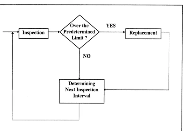
From the above literature review, a typical CBM procedure can be summarized in a diagram in figure 2.1. CBM is carried out first by performing an inspection on the maintained assets, then the asset condition is compared with the predetermined limit, if it is over the limit, the asset is going to be replaced with a new one (sometimes a rebuilt one) and the interval of next inspection is determined, otherwise the asset remains in service and the interval of next inspection is determined. As we can see the CBM

asset can obtained from the inspection (1) directly; (2) with 100 percent accuracy. For the second assumption, we just had a discussion of sensitivity and specificity in the last section. As the first assumption concerned, it sometimes may not be true. For example, in the case of freight car trucks, the internal condition of truck can not be inspected directly due to the nature of rail car structure, in this case, we have to develop some statistical models to estimate internal conditions by inspecting external components of freight car truck. This issue is going to be discussed in detail in next chapter.

Chapter 3

Inspection Approach to Support the Application of CBM

in Freight Car Trucks

Freight car trucks are an important component of rail vehicles, affecting the dynamic performance in ways that can have economic impacts on the track, vehicle and lading [Guins and Hargrove, 1994], and present a useful example of many of the

problems associated with developing and implementing an effective CBM program. In this chapter, first, the basic structure of three-piece freight car truck is reviewed. This is followed by a discussion of external and internal inspection of freight car trucks. Finally, inspection approaches to support CBM is presented.

3.1. Three - Piece Freight Car Truck and Inspection 3.1.1. Overview

From an engineering point of view, the entire subject of railway system can be thought as the interaction between train and track [cf. Hay 1982], or train-track system. A train-track system is comprised of three parts, the car body, the truck and the track, as shown in figure 3.1.

Freight car trucks provide the means for both support of the car body and the mobility of the freight car itself via steel wheels on steel rails. Four-wheel, three-piece

swivel trucks are the standard for American railway passenger cars and conventional freight cars (cf. Freight Car and Caboose Trucks, 1980). A three-piece freight car truck is

S4g be

sster

Source: Railroad Engineering, W. Hay, 1982.

Figure 3.1. Train-Track System

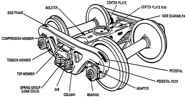
characterized by three types of parts: one truck bolster, two side frames and two wheelsets (Shown in figure 3.2, 3.3, and 3.4).

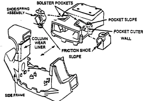
When the train moves, shock force and friction will happen to the car body and truck. To reduce the shock, a suspension system is designed and implemented for all types of car trucks. The system includes groups of springs carrying the load, a spring-loaded friction shoe and in some case hydraulic shock absorbers. The friction shoes fits in the bolster friction pocket (shown in figure 3.5 and 3.6).

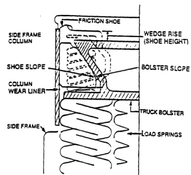
To dampen undesirable motions including vertical, lateral, longitudinal, rotational or any combination of such movements, several built-in mechanical friction liners, or plates, are designed and equipped on the freight car truck. Three types of liners are important in the later discussion of external condition and measurement, i.e. column wear liner, pocket wear liner and roof pedestal liner (shown in figure 3.5 and 3.6). The column wear liner is located between the inner side wall of the column and the outer side of the friction shoe. When the bolster moves up and down, the outer side of the friction shoes wears with the column wear liner instead of the inner wall of the column. The pocket wear liner is the liner located between the bolster pocket slope and the friction shoe. The roof pedestal liner is liner located between roof pedestal bearing adapter and truck sideframe. More detailed description about these two liners is given in the following chapters.

The bolster center plate not only functions as a pivot for the car body, but also carries the entire car body and loading weight into the truck structure. Although only a small rotating motion is sufficient in the center plate to permit trucks to negotiate even the sharpest curves, much concern is given to the plate's inner surface. Currently, the

CNT~ER PRATT SlOE

COMPRES

TENSI

COLUM BEARING

Source: ASF Maintenance and Repair Manual. Super Service Ride Control and Ride

Control Trucks. 1994.

Figure 3.2 Three-piece Freight Car Truck

BE ARING PAD

PEDESTAL

-. '. 10---2--- tO ...--- i - L- t--1'~.4 7 23 ·19 29-2 31 1f 32 I ... .

CRONT S1CE ELEVATION PVt 1YM SrRING SEAT I

POCAT y ". NSG-1 SF.AT I

( RAT TYP SPesG SUATI

j; 2+, 25

2 !

sorton rw

1. Top Momber Canter 2. Compression emoers

3. Com*ressson emoer Flanges

4. Sotm Center 5. Cagona Ternsrn

6. Tensmr Memoer F'anges 7. Coumnm

8. C.•,wm Flanges

9. Windows

10. Too Ends

11. Inner Sides a Cowumn

12. Lowr Bolster O••ning

13. Sp•ng Seat Fanges 14. Sprinq Seat Ribs

15. Journal Sacat Flanges 16. Reainer Key Slot

17. Inner Pedesta Legs

18. Pedese Root Wear Lner

19. Outer Pebestu Lags

20. Botstar Ano-Rotao•n Lugs

21. Parwng Le-Too Memeer 22. Too End Ocenrigs 23. Unit Bracxat

24. Botom Center Orain Hdes

25. Par:ng uL.,e-Bo o= Memr

26. Pedesa Root Wear wner Bostes

27. Too Wemoer &idge

28. Wear Plat Retaner Hole 29. car= Face

30. Coku=n Wear nmer 31. Sprnng Seat

32. Spring Seat Bosses or Lugs 33. Sorin Seat Orain Hoes 34. Bot•= Center Rib

Source: ASF Maintenance and Repair Manual. Su:per Service Ride Control and Ride Control Trucks. 1994.

23

/S •9

TOP VIEW

SECTION A-A

SIOE ELE;ATION

SOTTOM E;v ALTERNATE

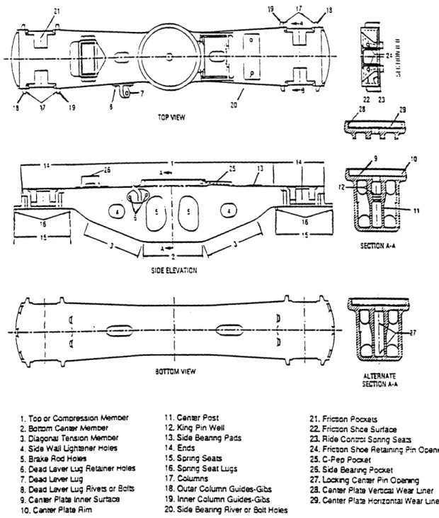
SECTION A-A 1. Too or Comoression Memoer

2. Bottm Center Meemoer

3. Diagorna Tension Memoer

4. Side Wall Ughtener Holes

5. Brake Rod Hotes

6. Dead Lever Lug Retainer Holes

7. Dead Levwe Lug

8. Dead Lever Lug Rivets or Bofs

9. Cener Plate inner Surtace

10. Canter Plate Rim

11. Cener Post

12. King Pin Well

13. Side 8eanng Pads 14. Ends

15. Spring Seats

16. Spnng Seat Lugs

17. Columns

18. Outer Column Guides-Gbs 19. Inner Column Guides-Gibs 20. Side Bearing River or BSot Holes

21. Fricton Pocxats

22. Fricoon Shce Surtaoe

23. Ride Conrr Sonng Seas

24. Fricton Shoe Retanne Pin Ocenrncs

25. C-Pep Pocxet 26. Side Bearuin Pocket

27. Locking Center Pin Ooeang

2~ Center Plate Verca Wear Uner 29. Center Plate Horizontal Wear Uner

Source: ASF Maintenance and Repair Manual, Super Service Ride Control and Ride Control Trucks, 1994.

)CKET SLOPE

POCKET CUTER

WALL

Source: Technical Papers. 1990 ASMEIIEEE Joint Railroad Conference.

Figure 3.5 Suspension System

SIDE FRAMI COLUMN SHOE SLOI COLUMN WEAR UNI SIDE FRAME GE RISE )E HEIGHT) TER SLCPE BOLSTER SPRINGS

Source: Technical Papers. 1990 ASMEIIEEE Joint Railroad Conference.

center plates for freight cars consist of casted inner surfaces covered by two abrasion resistant elastomeric center plate liner, i.e. bolster vertical wear liner and bolster

horizontal wear liner. These two liners are also described in more detail in the following chapter.

3.1.2. External Condition and Inspection

External condition refers to the condition of external parts that can be inspected without taking the car body off. The purpose of inspection on freight car truck is to prevent potential failures. There are several levels of failures caused by different type of truck defect. If some components of truck, such as truck spring, side bearing, pedestal thrust lugs, and friction wear plate, have excessive wear, then rail car may still be able to move, but will not be as smooth as it should be. This will cause high operating cost, damage to the freight. Thus such car has to be take out off service, normally classified as "bad order." On the other hand, if some of major components of truck, such as side frame of bolster, has a serious crack or is broken, then it may cause some serious consequences, such as derailment.

There are two types of external inspection. One type of external inspections of freight car trucks are performed in train yards upon train arrival or before train departure. Another type of external inspections are performed in the car shop after cars are taken to the car shop for "bad order" due to various damages.

When inspection is performed in the railroad yard, inspectors inspect side frame, wheels, and suspension system. These inspections are normally a combination of visual

inspection of surface of truck and gages' measurement of certain components. A defective freight car will be marked as a bad order and will be taken out of service.

According to AAR Railroad Freight Car Safety Standard, Rule 215.119, A railroad may not place or continue in service, if the car has

-(a) A side frame or bolster that -(1) Is broken, or;

(2) Has a crack of 11/4" of an inch or more in the transverse direction on a tension member.

(b) Spring assembly solid or snubber broken or missing. (c) A side bearing in any of the following conditions:

(1) Part of the side bearing assembly is missing or broken;

(2) The bearings at one end of the car, both sides, are in contact with the body bolster (except by design);

(3) The bearings at one end of the car have a total clearance from the body bolster of more than 3/4 of inch;

(d) Truck springs

(1) That do not maintain travel or load; (2) That are compressed solid; or

(3) More than one outer spring of which is broken, or missing, in any spring cluster;

A side frame or bolster can be damaged by coming in contact with an obstruction or by a rigid truck ( _{often caused by no side motion due to defective center plate, broken}

Once a car is placed as a bad order for its defective truck, it will be taken into a car shop, further inspection for external parts are performed. According to AAR Specification, inspect, gage and repair side frames as follows:

A. Column Guides

1. Inspect column guides for wear and gouges. Nominal column width is 71/2", if column is worn in excess of 1/8", side frame must be

reconditioned per AAR Specification M-214.

2. Inspection rotation stops on side frame inner column. Nominal distance between rotation stops in 17 3/16", if this dimension exceeds 17 33/8", side frame must be reconditioned per AAR Specification, M-214.

B. Pedestal Thrust Lugs

1. Gage longitudinal thrust lug wear according to AAR S-378. Nominal distance between thrust lugs is 7 1/4", if longitudinal distance between thrust lugs is not more than 7 1/2" and wear does not effect wheel base, i.e. wheel base matches the buttons as originally manufactured, no repair is necessary. If repair is necessary for either of the above reasons, side frame must be reconditioned per AAR Specification M-214.

2. Check width of pedestal thrust lugs. Nominal width is 3 1/2", if width is reduced below 3 33/8", side frame must be reconditioned per AAR Specification M-214.

C. Friction Wear Plates

1. Measure distance between side frame and column wear plates.

Nominal dimension is 14 1/2 ", if distance between wear plates exceeds 14 11/16" at any point, or if wear plate is cracked or broken (other than cracked retaining welds which may be rewelded) both column wear plates must be removed and new wear plates applied using mechanical fasteners per AAR Specification S-320 or S-3003. D. Pedestal Roof

1. Remove any existing roof liners and prepare pedestal rooffor application of "Transdyne" roof liners according to the manufacturers instructions.

3.1.3. Internal Condition and Inspection

We have discussed train-track system in which truck bolster contact with car body through the truck center plate bowl. As shown in figure 3.1, the condition on the central truck bolster areas cannot be inspected directly without taking the car body off. Therefore it is referred as internal condition in this study. The related parts are referred to as

internal parts. Among all the internal parts of a truck, the center plate bowl is the most vulnerable part and its condition affects the quality of the movement of car body directly.

As we described in the last section, further external inspection is performed once a car is dispatched to a car shop for bad order. After the external inspection, a responsible car shop engineer will decide whether to disassemble the car (lifting the car body off the

truck) and to inspect internal parts. If the engineer suspects that there may be some defects in the center plate bowls based on the external conditions, then he/she will decide to do so.

The judgment is mostly based on engineers experience and may be subject to two problems. One is the overestimation of the condition of wear of internal parts, and other is the underestimation. Each situation is associated with certain consequence and cost. If the wear condition for a truck is overestimated, then the truck will be disassembled even though the truck internal condition is still good. This will cause the cost associated with disassembling the truck, the cost for the loss of service time, or even the cost of market shares due to lack of car resource. On the other hand, if the case is underestimation, even though the internal condition of a truck is very poor, it will still be kept in the service, then the potential failure may happen, which is associated with certain cost. This is a critical issue when applying CBM to freight car trucks, which will lead to more study in next section.

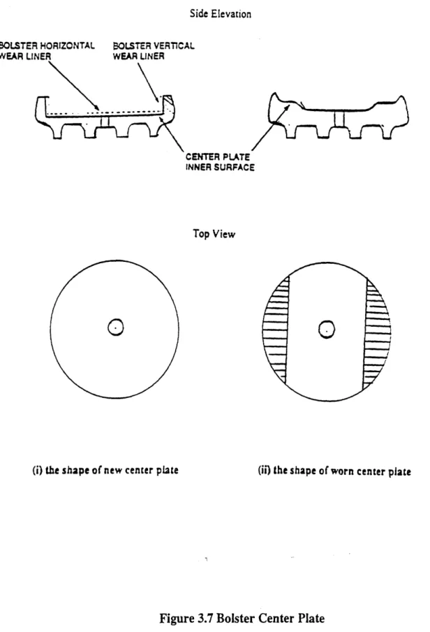
In practice, there is no single measurement of center plate applied to determine the internal condition of truck. Instead, a combination of wear measurements of center plate liners is used. Once the car body is taken off the truck, inspectors are supposed to do the following according to American Association of Railroad (AAR) Specification M-214:

1. Measure depth of center plate bowl. Nominal dimension is 1 1/8", if depth

exceeds 1 11/32 ", bolster must be reconditioned per AAR specification M-214. 2. Measure diameter of center plate bowl, if bowl diameter exceeds 14 1/4 " at any

58/8" at any point, entire bolster must be reconditioned per AAR Specification M-214.

Side Elevation BOLSTER HORIZONTAL BOLSTER VERTIC,

WEAR LINER WEAR LINER

CENTER PLATE

INNER SURFACE

Top View

(i) the shape of new center plate (ii) the shape of worn center plate

Figure 3.7 Bolster Center Plate

3.2. Inspection Approaches to Support CBM

As discussed in chapter 2 and also illustrated in figure 2.1, the starting point for CBM is the determination of the true condition. To apply CBM to rail car trucks, the true condition of truck internal parts, especially the condition of center plate bowl, is needed.

Unfortunately, the internal component is not accessible without taking car body off the truck. In practice, railroad car shop engineers tend to estimate the internal

conditions of a truck based on some of external conditions and their experience, which is not very accurate. Chang [1995] has attempted to address this problem by applying two statistical forecasting techniques, discrete choice method and performance threshold method, to develop a more effective inspection approach.

It is necessary to describe the underlying rationale for this proposition, which is to predict the internal condition of rail car truck from the external condition. Since the three-piece freight car truck is a complex mechanical system, the performance and wear

conditions of the different parts are likely to be interactive and integrative from one to another. Internal bolster is the only place taking all the weight of the car body and the freight loading, and all the forces are transmitted throughout the truck, especially the external area. Therefore, external conditions to some extent should be expected to reflect the overall performance of the internal bolster parts. This concept supports the predictive inspection approach for the internal bolster condition.

The idea is as follows. First, both data for internal condition and external condition are collected. Second some mathematical relations between internal and external condition are established by applying statistical data modeling techniques.

Finally, the internal condition of a car truck is predicted based on its external condition. The data could be collected in the railroad car shop where cars are maintained.

The author of this thesis has conducted further research in applying statistical modeling techniques to predict internal condition of a truck by inspecting its external components. In Chang's work, two types of statistical modeling techniques were analyzed and calibrated into the models, some data from a rail carrier was applied in those two models, but only moderate results were obtained. The two models were able to accurately predict the internal state of the truck approximately only 55-60% of the time. There were a number of reasons that were responsible for the results, which will be discussed in detail later, one of them was that data were not complete. In order to improve the

modeling results, the author has reviewed the data with railroad managers from one of the major north American railroads. We also collected more data from the railroad car shop, and applied to undated versions of models.

In this section, first, statistical forecasting techniques are reviewed, then results from both previous work and author's continued research are presented.

3.2.1. Review of Statistical Forecasting Techniques

Two statistical forecasting methods are presented in Chang's research, i.e., discrete choice method and performance threshold method.

3.2.1.1. Discrete Choice Method

In discrete choice method, dependent variable has a value from a set of alternatives or choices, instead of continue value as in linear method. Discrete choice

method seeks to find the link between the probabilities of dependent variable and independent variables.

Discrete choice method is rooted from random utility theory. Utility is the term used by economists to describe the level of satisfaction or happiness derived from the consumption or use of a good or service. According to classical consumer theory in microeconomic analysis, every consumer or user will choose the alternative or choice with the largest utility across the choice set. In random utility theory, the utility is

considered to consist of two parts, first part is called systematic factor, and second part is called random factor. For systematic factor, there are two types of independent variables. One is the attributes of each alternative. In the case of transportation mode choice

analysis for freight shippers, in which shippers select a particular mode from a set of alternatives or choices i.e., rail, truck, intermodel, delivery time (days), freight rate (dollar per unit), reliability (on time rate) and safety and damage (damage rate) of each mode are applied. The other one is the shipper's socioeconomic characteristics, e.g., the size of the shipper, the cost structure of the shipper and the nature of freight to be transported. The random part of a utility is account for all the factors that influence the decision of choice but are unobservable or unexplainable. A example of utility for transportation mode choice is [Ben-Akiva and Lerman, 1985],

uM

=

Po

+

X'

+

+

2

Px

3

3X1k

+.

+

+ '

=

v' + ',

S=

+ PX2

(31)

u = Po + x +

•x

+

+.+

x +

3

33

+ E

where:

SU u1, 2 and U3 are the utilities of the modes rail, truck and intermodal for the

shipper respectively;

* Io, 1, , 2, P3, "" -Pk are unknown parameters which are to be estimated by

discrete choice models;

* xli, x2i, x3i, ... Xk' (i=1,2,3) are the variables of the alternative's attributes and

shipper's socioeconomic characteristics for each alternative i, e.g. x1', x21, x3'

are transit time of the three modes;

* v , v2 _{and v}3 _{are the systematic components; and}

*

Because the utility of each alternative has a random term, any of them may have the highest utility, thus every alternative has some possibility to be chosen. In above case, the probability for a shipper to choose rail (mode 1) over truck (mode 2) or intermodal (mode 3) is,

Pr(mode 1) = Pr( u 2> u2 and u' 2 u3). (3.2)

More generally, alternative i would be chosen with the probability,

In order to be able to calculate the probability for each mode, more concrete specification of the distribution of the random term must be made. The most frequently used specification is Gumbel distribution (Johnson and Kotz (1970) and Domencich and McFadden (1975)), which can be expressed as,

f(s)

= ge

_"

_`

_{exp[-e-E"O'-],}

_(3.4)

where g and rl are two parameters. If the random term is assumed Gumbel distribution, then the difference between random terms associated with two modes e' -

&

Pr(i)

=

Pr(u' >

u')

for all j

i

ev

i

e

=

j-=1

In other words, the probability of alternative i being chosen is equal to the proportion of the exponential value of alternative i's utility to the summation of the exponential values of all the alternatives' utilities.

In the case of freight car truck, if we categorize the internal condition by the repairs done around center plate area, and define the internal condition with several states, e.g. "good", "OK" and "bad", according to some criterion about the repair work (for example, in Chang's work, if the type of work being done to a truck is nothing or rewelding of bolster vertical wear liner(BVWL), then the internal condition of this truck is categorized to state "good"; if the BVWL is rewelded and the bolster horizontal wear liner(BHWL) is replaced, then the internal condition of this truck is categorized to state "bad"; if BVWL is replaced, then the internal condition of this truck is categorized to state "poor". Then we can apply discrete choice method to predicting the internal

condition of rail car truck from its external conditions. There are some analogous aspects between predicting freight car truck internal condition and the above freight mode choice example. Pre-defined states of internal bolster condition are considered as the alternative choices and the external measurements the independent variables. Similar to the concept "utility", Chang used "tendency" in the freight car context. Then the tendencies for three internal states are defined as follows,

T

=

+ x

_+ax

₊

_{x +---ax}

₊

_E

₌

_d'

_+E'(3.6)

T2 _{= o + + cx 2 2 + k}

_X

_{+ E}

=d2

_(3.6)

T

_{=a +ax3}

₊₃

_=d

₊

_E,

where T' are the tendencies of internal condition being in state i; xki _{are the conditions of}

external components (i=1,2,3), d', d2 _{and d}3 _{are systematic components of the tendencies,}

The probability being in state i is the probability that the tendency to be in state i is larger than the tendency to be in any other state j. This can be expressed as,

Pr(i) = Pr(T

_{> T') for all j # i}

edt

=

d d' d'

(3.7)

edl + ed " +

e

ed'

Even though we have shown that there is similarity between the discrete choice analysis in the context of freight modes and freight car truck internal conditions, some differences still exist. One is that discrete choice model for freight modes is based on traditional consumer utility theory, a strong causal relationship is known to exist between utilities and the attributes of alternatives and the shipper's socioeconomic characteristics. On the other hand, it is clear that the external condition is not causal of the internal state, and the internal states, as defined, have somewhat of an arbitrary character. The internal states and external measurements are more likely to be different indices of the truck's overall performance and condition. Another difference is how the state(choice) is defined in two cases. Alternative shipping modes are absolutely discrete while internal condition is categorized into several states according to some essentially artificial criteria. This problem leads to the application of performance threshold method, which is to address this weakness.

3.2.1.2. Performance Threshold Method

As discussed earlier, the reason of to predict internal condition is to help railroad car shop manager make an effective decision on whether the car body is taken off and then whether the center plate liners is rewelded or replaced. The internal condition could be ideally a continuous measure, but what is needed is a series of ordinal states that corresponding varied decisions discussed above.

In 1975, Mckelvey and Zavoina proposed a statistical method called ordinal probit method in general econometric terminology, to apply in the situations that in many

statistical inference applications, the dependent variable, which is otherwise essentially continuous, falls in some ordinal levels of intervals. The freight car internal condition prediction may be considered as a case of this. In Chang's work, this method is called performance threshold method due to its application to the machinery inspection context. To be consistent, it is continuously referred as performance threshold method throughout this thesis.

With the same assumption of discrete choice model that the internal truck

condition can be indicated by its external condition, the performance function consists of two parts, i.e., a systematic and a random part. The performance function can be shown as follows [Chang 1995],

K

P = 1 k ,,n, + _(3.8)

k=1

where Pn is the performance of internal area of truck n; xkn is the kth external