Cost-Precision Tradeoffs in 3D Air Pollution Mapping using WSN

HAL Id: hal-01312940

https://hal.inria.fr/hal-01312940

Submitted on 9 May 2016

HAL is a multi-disciplinary open access

archive for the deposit and dissemination of

sci-entific research documents, whether they are

pub-lished or not. The documents may come from

teaching and research institutions in France or

abroad, or from public or private research centers.

L’archive ouverte pluridisciplinaire HAL, est

destinée au dépôt et à la diffusion de documents

scientifiques de niveau recherche, publiés ou non,

émanant des établissements d’enseignement et de

recherche français ou étrangers, des laboratoires

publics ou privés.

Cost-Precision Tradeoffs in 3D Air Pollution Mapping

using WSN

Ahmed Boubrima, Walid Bechkit, Hervé Rivano, Lionel Soulhac

To cite this version:

Ahmed Boubrima, Walid Bechkit, Hervé Rivano, Lionel Soulhac. Cost-Precision Tradeoffs in 3D Air

Pollution Mapping using WSN. UNET 2016 - 2nd International Symposium on Ubiquitous Networking,

May 2016, Casablanca, Morocco. �hal-01312940�

Cost-Precision Tradeoffs in 3D Air Pollution

Mapping using WSN

Ahmed Boubrima1_{, Walid Bechkit}1_{, Hervé Rivano}1_{, and Lionel Soulhac}2

1

Univ Lyon, Inria, INSA Lyon, CITI, F-69621 Villeurbanne, France

2

LMFA, Univ Lyon, CNRS UMR 5509 ECL, INSA Lyon, Univ Claude Bernard, 69134 Ecully, France

Abstract. Air pollution has become a major issue of modern megalopo-lis, where the majority of world population lives. Measuring air pollution levels is an important step in designing and assessing air quality related public policies. Unfortunately, existing solutions are inadequate to get insights on the real exposition of citizens. In particular, high quality sensors deployed today are too large and too costly to envision a three dimensional deployment at the scale of a street. In this paper, we investi-gate the deployment of wireless sensor networks (WSN) used for building a three-dimensional mapping of pollution concentrations. We consider in our simulations a 3D model of air pollution dispersion based on real ex-periments performed in wind tunnels emulating the pollution emitted by a steady state traffic flow in a typical street canyon. Our contribution is to analyze the performances of different 3D WSN topologies in terms of the trade-off between the economical cost of the infrastructure and the quality of the reconstructed air pollution mapping.

1

Introduction

Air pollution affects human health dramatically. According to the World Health Organization (WHO), exposure to air pollution is accountable to seven million casualties in 2012 [15]. In 2013, the International Agency for Research on Cancer (IARC) classified particulate matter, the main component of outdoor pollution, as carcinogenic for humans [14]. Air pollution has become a major issue of mod-ern megalopolis, where the majority of world population lives, adding industrial emissions to the consequences of an ever denser urbanization with traffic jams and heating/cooling of buildings. As a consequence, the reduction of pollutant emissions is at the heart of many sustainable development efforts, in particular those of smart cities. Monitoring urban air pollution is therefore required by both municipalities and the civil society to develop pollution mitigation public policies.

Current air quality monitoring is mostly operated by independent authorities. Conventional measuring stations are equipped with multiple lab quality sensors [13]. These systems are however massive, inflexible and expensive. An alternative – or complementary – solution would be to use wireless sensor networks (WSN) [7] which consist of a set of lower cost nodes that can measure information from

the environment, process and relay them to some base stations, denoted as sinks [17]. The progress of electrochemical sensors, that are smaller and cheaper while keeping a reasonable measurement quality, makes the use of WSN for air quality monitoring viable [10]. The main advantage of the use of WSN for air pollu-tion monitoring is to obtain a finer spatiotemporal granularity of measurements, thanks to the resulting lighter installation and operational costs [11]. Although some WSN-based air quality monitoring systems are already operating [3,4,8], the deployment issue of these tiny nodes while taking into account the precision of the resulting network has not yet been investigated.

Minimizing the deployment cost is a major challenge in WSN design. The problem consists in determining the optimal positions of sensors and sinks so as to cover the environment and ensure network connectivity while minimizing the deployment cost [19]. The deployment is constrained by the cost of the nodes and sinks, but also by operational costs such as the energy spent by the nodes. The network is said connected if each sensor can communicate information to at least one sink [18]. The coverage issue has often been modeled as a k-coverage problem in which at least k sensors should monitor each point of interest. Most research work on coverage uses a simple detection model which assumes that a sensor is able to cover a point in the environment if the distance between them is less than a radius called the detection range [2]. This can be true for some applications like presence sensors but is not suitable for pollution monitoring. Indeed, a pollution sensor detects pollutants that are brought in contact by the wind. The notion of detection range is thus irrelevant in this context. Therefore, a deployment model is still needed for the air quality monitoring application.

In this paper, we investigate the deployment of wireless sensor networks (WSN) used for building a three-dimensional mapping of pollution concentra-tions. We base on interpolation methods to evaluate the accuracy of a given wireless sensor networks topology. Then, we present an optimization model for optimal air pollution mapping. We consider in our simulations a 3D model of air pollution dispersion based on real experiments that we have performed in wind tunnels. Our contribution is to analyze the performances of different 3D WSN topologies in terms of the trade-off between the economical cost of the infras-tructure and the quality of the reconstructed air pollution mapping in terms of precision.

The remainder of this paper is organized as follows. First, we review in section 2 the most used methods in the estimation of air pollution concentrations. Then, we present in section 3 the formulation used for assessing the accuracy of a given WSN topology. After that, we present the simulation data set and the obtained results in section 4. Finally, we conclude and give some perspectives in section 5.

2

Air pollution mapping

As claimed in the introduction, our goal is to evaluate how much the estimation of pollution concentrations by a given WSN topology is good. Air quality estimation

allows to determine pollution concentrations of locations where no sensor is deployed, and this based on pollution concentrations gathered by the deployed sensors [9]. Three major methods are used to do so: atmospheric dispersion, interpolation and land-use regression [6].

Atmospheric dispersion models take as input locations of pollution sources, the pollutant emission rate of each pollution source and meteorological data in order to measure the pollutant concentration at a given location [6]. The obtained concentrations can then be calibrated using the measurements of sensors.

Interpolation methods formulate the estimated concentration bZp at a given

location p ∈ P as a weighted combination of the measured concentrations Zq, q ∈

P −{p} [16]. The weights of the measured concentrations Wpqcan be evaluated in

a deterministic way based on the distance between the location of the measured concentration and the location of the estimated concentration. In this case, which is called the Inverse Distance Weighting interpolation, bZp is evaluated using

formula 1. The concentration weights can also be evaluated in a stochastic way, the most used method doing so is called kriging.

b Zp= P q∈P−{p}Wpq∗ Zq P q∈P−{p}Wpq (1) The last method is land-use regression models, which are a kind of stochastic regression models [5]. The idea behind these models is to evaluate the pollution concentration at a given location based on the concentrations of locations that are similar in terms of land-use parameters such as the elevation and the distance to the closest busy road.

In the next section, we present the placement model allowing to determine sensor optimal positions in such a way that the estimation error is minimized, and hence evaluate the trade-off between the number of sensors and the ac-curacy of the reconstructed pollution map. In order to design our air quality coverage formulation, we use the so-called inverse distance weighting interpola-tion as interpolainterpola-tion method. Our choice is motivated by the fact that in this latter, weights are given in a deterministic way, which allows to integrate them into the ILP deployment model.

3

Optimization model of pollution mapping

3.1 Inputs and objective function

We consider as input of our model the map of a given urban area that we call the deployment region. We start by discretizing the deployment region in order to get a set of points P approximating the urban area at a high-scale (|P| = N ). Our goal is to be able to determine with a high precision the concentration value at each point p ∈ P . We ensure that for each point p ∈ P , either a sensor is deployed or the pollution concentration can be estimated with a high precision based on the data gathered by the neighboring deployed sensors.

In general case, the set P is thus considered as the set of potential positions of WSN nodes. However, in smart cities applications, some restrictions on node positions may apply because of authorization or practical issues. When this is the case, we do not consider as potential positions the points p ∈ P where sensors cannot be deployed. We use decision variables xpto specify if a sensor is deployed

at point p or not. All the potential positions of sensors are supposed linked to the base station, thus we focus only on the constraint of pollution mapping. The objective function to minimize is thus given as follows.

F =X

p∈P

xp (2)

3.2 Constraints

Using numerical atmospheric dispersion models, we first get simulated pollution concentrations that may be considered as reference pollution concentrations. This does not mean that these reference concentrations are real but they reflect the best today’s pollution knowledge. Let Zpdenote the reference concentration

value at point p. Given the set of selected points where sensors will be deployed {p where xp = 1}, we evaluate the estimated pollution concentrations bZp at

points {p where xp= 0} based on reference values corresponding to the selected

points, i.e. based on Zp where p ∈ {p where xp= 1}, as follows.

           b Zp= P q∈P−{p}Wpq∗ Zq∗ xq P q∈P−{p}Wpq∗ xq , p ∈ P & xp= 0 X q∈P−{p} Wpq∗ xq> 0, p ∈ P & xp= 0 (3)

We ensure that the denominator of bZpis never equal to zero using the second

part of (3). The Wpq parameter is the correlation coefficient between points p

and q and is calculated using (4) based on the distance between the two points. D(p, q) is the distance function. α is the attenuation coefficient of the correlation distance, this means that for greater values of α, very low correlation coefficients are assigned to far points. The last parameter of (4) is the maximum correlation distance, which defines the range of correlated neighboring points of a given point.

In order to take into account the impact of the urban topography on the dispersion of pollutants, let D be the shortest distance along the roads network. This allows to assign small correlation values to points that are separated by buildings, even if they are close.

Wpq=    1 D(p, q)α if q ∈ Disc(p, d) − {p} 0 if q /∈ Disc(p, d) (4)

In order to ensure that the concentration is estimated with high precision at points where no sensor is deployed, we introduce the constraint (5). The Ep

parameter corresponds to the estimation error that is tolerated at point p. The choice of different values of Ep in function of p allows to assign low tolerated

estimation errors to locations that are sensitive to air quality such as hospitals, primary schools, etc.

  Zbp− Zp   ≤ Ep, p ∈ P & xp= 0 (5) By replacing bZp by its expression given in (3), we obtain the coverage

con-straints (6) and (7).      P q∈P−{p}Wpq∗ Zq∗ xq P q∈P−{p}Wpq∗ xq − Zp      ≤ Ep, p ∈ P & xp= 0 (6) X q∈P−{p} Wpq∗ xq> 0, p ∈ P & xp= 0 (7)

4

Simulation Results

The constraints introduced in the previous section can be linearized in order to obtain an Integer Linear Program. The details of the linearization are presented in [1]. The resulting ILP takes as an input a set of potential positions for the deployment of sensors, a set of points where the error of estimation has to be bounded and the ground truth of pollution concentrations. The output is the topology of the minimum cost wireless sensor network respecting the bound on pollution estimation error.

In the following, we first describe the ground truth taken as input, generated in an experimental wind tunnel emulating an actual street canyon. We then study the cost-precision trade-off in three different ways. We focus on a vertical plan and show the impact of the targeted precision on the cost of the infrastructure. We also investigate the impact of the quality of sensors, which is an important cost-factor of the devices. We then constrain the deployment to achievable posi-tions in a urban area and limit the evaluation of the precision at posiposi-tions where people may be exposed to the pollutants. We finish by investigating the impact of a longitudinal variation of the pollution concentration on the cost of a full 3-dimensional deployment of sensors.

4.1 Ground truth pollution concentration in a street canyon

When studying city scale, 2-dimensional deployments of sensors, one can take as input historical data of pollution dispersion over the map of the city [1]. In order to evaluate the cost-precision trade-off for a 3 dimensional mapping of

the pollution concentrations in a street, a more detailed dataset is required. In particular, the vertical dispersion of the pollutants has to be known.

The ground truth that are used in this paper are measurements generated in an instrumented wind tunnel test bed. The experimental set up emulates a street canyon described in Fig. 1. The emulated street is 100m long (Y axis, coordinates in [−50, 50]), 20m large (X axis, [−10, 10]) and 20m high (Z axis, [0, 20]). The details on the wind and pollutant emissions as well as the physics involved for scaling the measurements on the wind tunnels into the pollution concentrations on the emulated street are found in [12]. The pollution emissions of a steady state urban vehicular traffic is emulated along the longitudinal (0, Y, 0) axis, the wind being perpendicular to it. The pollution concentrations are constant along this dimension. Sensors are deployed in the vertical (X, 0, Z) plan.

Fig. 1: Wind tunnel set up and measurements in the (X, O, Z) plan [12].

The ground truth concentrations that are considered in our experiment are in the zone of interest depicted in Fig. 1: the square of the width of the street and 10m high that corresponds to the zone where people can be exposed and where pollution can get into the first two to three floors in apartments.

4.2 Precision cost on a vertical plan

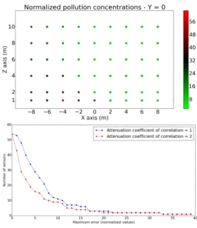
In this first scenario, we evaluate the cost-precision trade-off in the mapping of the (X, O, Z) vertical plan. The cost of the infrastructure is mainly the number of sensors to be deployed. The precision of the mapping is evaluated by the maxi-mum difference between a ground truth and the result of the linear interpolation of the deployed sensors measurements. Here, the set of potential positions for sensors and the set of points where the precision of the mapping is evaluated are the same. They are the points of a 2-D regular grid over the zone of interest of the wind tunnel data set, as depicted in Fig. 2, together with the cost-precision trade-off obtained by our model.

As expected, the cost of the infrastructure decreases when the precision of the interpolation is more tolerated. Interestingly, increasing the attenuation of the correlation improves on the linear interpolation when a high precision is

required. As a matter of fact, when looked at a small scale, the diffusion pattern of the pollution is quite different from a linear field. With a weak attenuation in the linear interpolation, the values of the distant sensors have a too strong impact on the estimation, introducing errors, hence requiring a higher density of sensors. When a lower precision is required, the small variations on the lower-left side of the street (because of the wind direction in this scenario) fall within the error margin and the field of concentration values is closer to a linear one. Hence, the lesser impact of the attenuation.

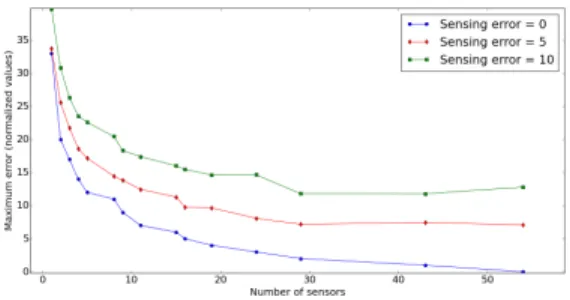
We now investigate the impact of sensing quality. If we assume that the sensors are accurately calibrated, one of the most important cost factors is the quantity of random errors that is added to the sensor’s readings and which depends on the quality of the power source and the electronic components of the sensor. In this simulation, we consider that these errors are a Gaussian noise of a mean «sensing_error». The impact of the sensing errors on the precision of estimation is depicted in Fig. 3. The impact of the sensing varies with the density of deployed sensors. When a sensor is deployed at each potential position, the maximum error of the estimation is the the raw sensing error. When the deployment is sparse, the maximum error combines the errors induced by the linear interpolation without considering sensing errors, plus the sum of the noises on the sensors contributing to the estimation. These noises being in this case less important than the interpolation errors, their impact on the maximum error is less significant.

Fig. 3: Quality of sensor vs precision.

4.3 Realistic deployment and citizen’s exposure

In practical situations, the sensors cannot be deployed at the potential positions used in the previous scenario. In order to deploy a sensor, one need a urban furniture or a wall. In the following, we restrict the potential positions to be at the vertical of sidewalks: no sensors are allowed on the roadway. Obviously, this will decrease the precision of the estimation.

On the other hand, the positions at which the precision matters are those that have an impact on the exposure of people. We therefore focus on the precision of the estimation on points lower than 2m (where someone is directly exposed), and points close to walls (since these are in interaction with buildings). The resulting set of potential positions is depicted in Fig. 4.

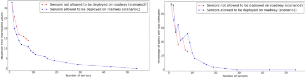
We depict the obtained results in Fig. 5, left hand side. As expected, the fact that no sensor can be deployed on the roadway increases the maximum error. The plot stops when the best achievable precision is reached: additional sensors do not improve the result. The maximum error obtained is high in particular because there is a peak of concentration on the roadway.

Another viewpoint on the quality of estimation is the proportion of the map-ping that is accurate. When communication about air quality toward citizens is at stake, actual values of pollution concentration are not given. Authorities prefer more readable "Air Quality Indicators" (AQI) which are some kind of discretization of the pollution concentration into classes. The results in Fig. 5 right hand side depict the percentage of points on which the estimation gives a wrong AQI. As expected, few exceptions apart, when the maximum absolute error decreases, the proportion of wrong AQI decreases also. More surprisingly, the restricted deployments gives less wrong AQIs. Indeed, if the positions on the roadway are prone to higher errors, there is only a small number of them.

4.4 3D mapping

In the following, we consider the impact of the variability of the pollution con-centration on the cost of the infrastructure required for producing a three di-mensional mapping.

Fig. 4: Meaningful positions for citizen’s exposure.

Fig. 5: Cost-precision tradeoff - focus on citizen’s exposure and reading.

We extend the 2D grid used in the previous scenario into a 3D one by con-sidering different planes along the Y axis. We consider 9 possible values for Y ∈ [−40, 40], i.e. a plane each 10m, in order to avoid the two ends of the street, where very different phenomenon may occur. Let S(x, y, z) be the concentra-tion value at point (x, y, z). The 2D grid used in the previous simulaconcentra-tion case corresponds to the concentrations at the center of the street, S(x, 0, z).

The dataset that is taken as input has been produced with homogeneous traffic assumptions. Consequently, pollution concentrations are constant along the longitudinal axis (Y ). In order to generate longitudinally varying concentra-tions, we use the sinusoidal model given in (8). This model is theoretical and does not claim to represent a real situation.

S(x, y, z) = (cos( y 40∗ φ) m + m − 1 m ) ∗ S(x, 0, z) (8)

Two parameters characterize the variation of pollution concentrations along the Y-axis, φ and m. The m parameter allows to define the range of the concen-trations: S ∈ [m−2

m , 1], m ≥ 2.

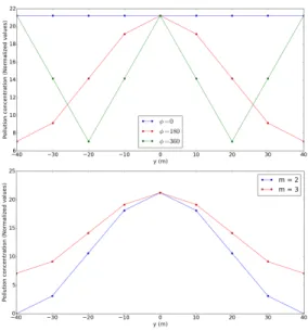
The φ parameter defines the variation of concentration from a plane y to a neighboring one. It somehow captures the presence of peaks in the production of pollutants where (8) takes maximal values as depicted in Fig. 6.

Fig. 7 depicts the number of optimally deployed sensors depending on pa-rameters φ and m for a given precision. Surprisingly, the situations requiring the

Fig. 6: Pollution vs φ (for m = 3) and m (for φ = 180) at point (x=0,y,z=2).

highest number of sensors to deploy are those when the pollution concentration varies the less: the scenarios with m = 3 cost more than those with m = 2, and when φ = 0, the concentration is constant along the Y axis. When φ = 360, the increase of the cost of infrastructure may be an artifact of the combination of the periodicity of the variation and the discretization of the space by the potential positions. Indeed, the values of the concentrations are constant on the positions in Fig. 6.

Fig. 7: Cost of a 3D deployment vs longitudinal variability.

The explanation of this phenomenon is yet to be confirmed and investigated. We conjecture that the reason comes from the isotropy of the correlation function in the interpolation. Indeed, in our case the Y axis is a very particular direction and the isotropy of the interpolation does not take that into account. In

partic-ular, the correlations in the X Z plans are different than the one in the Y axis. In a future work, we will investigate the integration of the bias induced by the urban environment in the interpolation function to improve on the cost-precision tradeoff.

5

Conclusion and future work

In this paper, we investigate the cost-precision tradeoffs in 3D air pollution mapping using wireless sensor networks. Our main contribution is the analysis of different WSN topologies, confronting their deployment cost – mainly the number of deployed sensors – and the accuracy of a linear interpolation of their readings to build a maps of pollution concentrations. We present and apply our deployment model on pollution concentrations obtained from a testbed made of wind tunnels, emulating the diffusion of the pollution emitted by a steady state traffic flow in a typical urban canyon. We show how the deployment cost evolve with the estimation error that is tolerated.

As a future work, we plan to improve our correlation function in order to take into account the bias induced by urban topography and weather conditions.

Acknowledgment

This work has been supported by the "LABEX IMU" (ANR-10-LABX-0088) and the "Programme Avenir Lyon Saint-Etienne" of Université de Lyon, within the program "Investissements d’Avenir" (ANR-11-IDEX-0007) operated by the French National Research Agency (ANR).

References

1. Boubrima, A., Bechkit, W., Rivano, H.: Optimal deployment of dense wsn for error bounded air pollution mapping. In: International Conference on Distributed Computing in Sensor Systems (DCOSS 2016). IEEE (2016)

2. Chakrabarty, K., Iyengar, S.S., Qi, H., Cho, E.: Grid coverage for surveillance and target location in distributed sensor networks. Computers, IEEE Transactions on 51(12), 1448–1453 (2002)

3. Devarakonda, S., Sevusu, P., Liu, H., Liu, R., Iftode, L., Nath, B.: Real-time air quality monitoring through mobile sensing in metropolitan areas. In: Proceedings of the 2nd ACM SIGKDD International Workshop on Urban Computing. p. 15. ACM (2013)

4. Hasenfratz, D., Saukh, O., Walser, C., Hueglin, C., Fierz, M., Thiele, L.: Pushing the spatio-temporal resolution limit of urban air pollution maps. In: Pervasive Computing and Communications (PerCom), 2014 IEEE International Conference on. pp. 69–77. IEEE (2014)

5. Hoek, G., Beelen, R., De Hoogh, K., Vienneau, D., Gulliver, J., Fischer, P., Briggs, D.: A review of land-use regression models to assess spatial variation of outdoor air pollution. Atmospheric environment 42(33), 7561–7578 (2008)

6. Jerrett, M., Arain, A., Kanaroglou, P., Beckerman, B., Potoglou, D., Sahsuvaroglu, T., Morrison, J., Giovis, C.: A review and evaluation of intraurban air pollution exposure models. Journal of Exposure Science and Environmental Epidemiology 15(2), 185–204 (2005)

7. Kumar, A., Kim, H., Hancke, G.P.: Environmental monitoring systems: a review. Sensors Journal, IEEE 13(4), 1329–1339 (2013)

8. Marjovi, A., Arfire, A., Martinoli, A.: High resolution air pollution maps in urban environments using mobile sensor networks. In: Distributed Computing in Sensor Systems (DCOSS), 2015 International Conference on. pp. 11–20. IEEE (2015) 9. Marshall, J.D., Nethery, E., Brauer, M.: Within-urban variability in ambient air

pollution: comparison of estimation methods. Atmospheric Environment 42(6), 1359–1369 (2008)

10. Mead, M., Popoola, O., Stewart, G., Landshoff, P., Calleja, M., Hayes, M., Baldovi, J., McLeod, M., Hodgson, T., Dicks, J., et al.: The use of electrochemical sensors for monitoring urban air quality in low-cost, high-density networks. Atmospheric Environment 70, 186–203 (2013)

11. Rajasegarar, S., Havens, T.C., Karunasekera, S., Leckie, C., Bezdek, J.C., Jam-riska, M., Gunatilaka, A., Skvortsov, A., Palaniswami, M.: High-resolution mon-itoring of atmospheric pollutants using a system of low-cost sensors. Geoscience and Remote Sensing, IEEE Transactions on 52(7), 3823–3832 (2014)

12. Salizzoni, P., Soulhac, L., Mejean, P.: Street canyon ventilation and atmospheric turbulence. Atmospheric Environment 43 (2009)

13. Air Rhône-Alpes: The air quality monitoring organization of the lyon agglomera-tion, http://www.air-rhonealpes.fr [2016-01-27]

14. International Agency for Research on Cancer: Iarc: Outdoor air pollution a leading environmental cause of cancer deaths, on http://www.iarc.fr/en/ media-centre/iarcnews/pdf/pr221_E.pdf [2016-01-27]

15. World Health Organization: Burden of disease from household air pollution for 2012, on http://www.who.int/phe/health_topics/outdoorair/databases/ FINAL_HAP_AAP_BoD_24March2014.pdf [2016-01-27]

16. Wong, D.W., Yuan, L., Perlin, S.A.: Comparison of spatial interpolation methods for the estimation of air quality data. Journal of Exposure Science and Environ-mental Epidemiology 14(5), 404–415 (2004)

17. Yick, J., Mukherjee, B., Ghosal, D.: Wireless sensor network survey. Computer networks 52(12), 2292–2330 (2008)

18. Younis, M., Akkaya, K.: Strategies and techniques for node placement in wireless sensor networks: A survey. Ad Hoc Networks 6(4), 621–655 (2008)

19. Zhu, C., Zheng, C., Shu, L., Han, G.: A survey on coverage and connectivity issues in wireless sensor networks. Journal of Network and Computer Applications 35(2), 619–632 (2012)