HAL Id: hal-03044722
https://hal.archives-ouvertes.fr/hal-03044722
Submitted on 15 Dec 2020
HAL is a multi-disciplinary open access archive for the deposit and dissemination of sci-entific research documents, whether they are pub-lished or not. The documents may come from teaching and research institutions in France or abroad, or from public or private research centers.
L’archive ouverte pluridisciplinaire HAL, est destinée au dépôt et à la diffusion de documents scientifiques de niveau recherche, publiés ou non, émanant des établissements d’enseignement et de recherche français ou étrangers, des laboratoires publics ou privés.
Integration Duration-Based Method for Unveiling
Hidden Patterns of Even Number of Spirals of Chua
Chaotic Attractor
Malika Belouerghi, Tidjani Menacer, René Lozi
To cite this version:
Malika Belouerghi, Tidjani Menacer, René Lozi. Integration Duration-Based Method for Unveiling Hidden Patterns of Even Number of Spirals of Chua Chaotic Attractor. Indian Journal of Industrial and Applied Mathematics, Indian Journals, 2019, 10 (1), pp.13-33. �10.5958/1945-919X.2019.00020.3�. �hal-03044722�
1
Published in: Indian Journal of Industrial and Applied Mathematics, Vol. 10, No. 1, Jan-June 2019, pp. 13-33. DOI: 10.5958/1945-919X.2019.00020.3
Personal file
Integration Duration-Based Method for Unveiling Hidden
Patterns of Even Number of Spirals of Chua Chaotic
Attractor
Malika Belouerghi
1, Tidjani Menacer
2and René Lozi
3*
1,2Department of Mathematics, University Mohamed Khider, Biskra, Algeria.
3University Côte d’Azur, CNRS, LJAD, Parc Valrose 06108, Nice Cédex 02, France.
(*Corresponding author) E-mail: *Rene.LOZI@univ-cotedazur.fr
1belouerghimalika@yahoo.fr, 2tidjanimenacer@yahoo.fr
Abstract: The purpose of this article is to introduce a novel method for unveiling hidden
patterns of even number of spirals in the multi-spiral Chua Chaotic attractor. This method is based on the duration of integration of this system and allows displaying every pattern containing from 1 to c+1 spirals of this attractor. After having given the equation of the multi-spiral Chua Chaotic attractor, the Menacer–Lozi–Chua (MLC) method for uncovering hidden bifurcations is explained again and a numerical example of a route of bifurcation is given. In the chosen example, the attractors found along this hidden bifurcation route display an odd number of spirals. With the novel method, during the integration process, before reaching the asymptotical attractor which possesses an odd the number of spirals, the number of spirals increases one by one until it reaches the maximum number corresponding to the value fixed by ε, unveiling both patterns of even and odd number of spirals.
Keywords: hidden bifurcation, Chua’s circuit, pattern of even number of spirals
INTRODUCTION
The name ‘bifurcation’ was first introduced by Henri Poincaré in 1885[1] in the frame of the qualitative theory of dynamical systems. A bifurcation occurs when, for a fixed value of a parameter, the number of solutions of a family of differential equations is increased from one to two, like the bifurcation of a branch of a tree[2, 3], or when the topological nature of the solution changes from steady state to periodic function (Hopf bifurcation[4]).
In 1963, the discovery of the first chaotic strange attractor by Lorenz[5] has broadened the field of the bifurcation theory. The first system of differential equation modelling real electronic device for which the asymptotic attractor is chaotic (hence a strange attractor) was invented by Chua[6] during a stay in the laboratory of professor Matsumoto, at Waseda University, Tokyo.
Chua attractor is nowadays incredibly used because both of its realisations: electronic circuit or system of differential equations can be combined for multiple purposes[7]. Chua circuit is the simplest electronic circuit exhibiting chaos and possesses a very rich dynamical
2 behaviour which was verified from numerous laboratory experiments[8], computer simulations[9] and rigorous mathematical analysis[10–12].
Since that discovery, the Chua circuit has been generalised to several versions. One generalisation substitutes the continuous piecewise linear function by a smooth function, such as a cubic polynomial[13–16], etc. Complex attractors with n-double spirals were reported in Suykens and Vandewalle[17] by introducing additional break points in the non-linear element in the Chua’s circuit or using cellular neural networks with a piecewise linear output function[18].
It is also demonstrated in Suykens et al. and Yalçin et al.[19, 20]; odd number of scrolls can be observed by a similar modification. In Tang et al.[21], it is shown that the n-spirals attractors can be obtained with a simple sine or a cosine function.
In 2011, Leonov et al. introduced a new classification of attractors of dynamical systems with the concept of hidden attractor and self-excited attractor[22, 23]. They showed that the
basin of attraction of a self-excited attractor overlaps with the neighbourhood of an equilibrium point; therefore, these attractors are very easy to be found, because it suffices to give the equilibrium point as an initial condition, if this equilibrium point is unstable. On the contrary, a hidden attractor has a basin of attraction that does not intersect with small neighbourhoods of any equilibrium points, thereby making it very difficult to find. The name hidden comes from this property.
Hidden attractors are important in engineering applications because they allow unexpected and potentially disastrous responses to perturbations in a structure like aircrafts control systems (windup and anti-windup) and electrical machines. An effective method for the numerical localisation of hidden attractors in multi-dimensional dynamical systems has been proposed by these Leonov and Leonov et al.[24, 25]. This method is based on homotopy and numerical continuation. They construct a sequence of similar systems such that for the first (starting) system the initial condition for numerical computation of oscillating solution (starting oscillation) can be obtained analytically. Then the transformation of this starting solution is tracked numerically in passing from one system to another. The first example of a hidden chaotic strange attractor was found in the Chua attractor[26].
In their study of the modified multi-spiral Chua system with sine function[21], Menacer et al.[27], using the Kuznetsov and Leonov method in another way, found a sequence of hidden bifurcations.
In this system, the parameter c governing the number of spirals is an integer; hence, it is not possible to vary it continuously and therefore it is not possible to observe bifurcations of attractors from n to n+2 spirals when the parameter c changes. Moreover, it is not possible to use non-integer real values for c. To overcome this obstacle, they introduced a new bifurcation parameter ε provided by the method of researching hidden attractor.
Next, in ‘Multiple-spiral attractors in Chua’s sine function system’ section, the multi-spiral Chua system with sine function is recalled. In ‘The Menacer–Lozi–Chua (MLC) method for method for uncovering hidden bifurcations’ section, the Menacer–Lozi–Chua (MLC) method for uncovering hidden bifurcations is explained again. In the chosen example, it shown that the attractors along the hidden bifurcation route display an odd number of spirals. In ‘Integration duration method for unveiling hidden patterns of even number of spirals’ section, we introduce a novel method for unveiling hidden patterns of even number of
3 spirals. This method based on the duration of integration of the considered system. During the integration process, before reaching the asymptotical attractor which possesses and odd the number of spirals, the number of spirals increases until it reaches the maximum number corresponding to the value fixed by ε. Finally, in ‘Conclusion’ section, a brief conclusion is drawn.
MULTIPLE-SPIRAL ATTRACTORS IN CHUA’S SINE FUNCTION
SYSTEM
Complex chaotic attractors with n-double scrolls using cellular neural networks with a piecewise linear output function were reported in Arena et al.[18]. In Tang et al.[21], a new family of continuous functions for generating n-scroll attractors is proposed. It is shown that n-scroll attractors can be obtained with a simple sine or cosine function. Since then in the last decades, multi-scroll chaotic attractors generation has been extensively studied due to their promising applications in various real-word chaos-based technologies including secure and digital communications, random bit generation and so on.
The system of differential equations, describing the behaviour of Chua’s circuits, is three-dimensional with a piecewise linear non-linearity[6, 28].
{ 𝑥̇(𝑡) = 𝛼(𝑦(𝑡) − 𝑓(𝑥(𝑡))) 𝑦̇(𝑡) = 𝑥(𝑡) − 𝑦(𝑡) − 𝑧(𝑡) 𝑧̇(𝑡) = −𝛽𝑦(𝑡) (1) with 𝑥̇(𝑡) =𝑑𝑥(𝑡) 𝑑𝑡 , 𝑦̇(𝑡) = 𝑑𝑦(𝑡) 𝑑𝑡 , 𝑧̇(𝑡) = 𝑑𝑧(𝑡) 𝑑𝑡
For the Chua’s modified system with a sine function, the non-linearity reads (Figure 1):
𝑓(𝑥(𝑡)) = { 𝑏𝜋 2𝑎(𝑥(𝑡) − 2𝑎𝑐), 𝑖𝑓 𝑥(𝑡) ≥ 2𝑎𝑐 −𝑏 𝑠𝑖𝑛 (𝜋𝑥(𝑡) 2𝑎 + 𝑑) , 𝑖𝑓 − 2𝑎𝑐 ≤ 𝑥(𝑡) ≤ 2𝑎𝑐 𝑏𝜋 2𝑎(𝑥(𝑡) + 2𝑎𝑐), 𝑖𝑓 𝑥(𝑡) ≤ −2𝑎𝑐 (2)
4 In this article, rather than considering the fractal structure of the attractors, we highlight their global geometric feature, that is, we only consider their general shape described in terms of the number of spirals. We fix the real parameter values 𝛼 = 11, 𝛽 = 15, 𝑎 = 2, 𝑏 = 0.2 for which one can find chaotic attractors topologically equivalent to the attractors described in Ref. [21].
The parameter c is an integer which governs the number n of spirals.
𝑛 = 𝑐 + 1 (3)
and d is chosen such that
𝑑 = {𝜋 𝑖𝑓 𝑐 𝑖𝑠 𝑒𝑣𝑒𝑛
0 𝑖𝑓 𝑐 𝑖𝑠 𝑜𝑑𝑑 (4)
A straightforward computation gives the equilibrium points which are (−𝑥𝑒𝑞, 0, 𝑥𝑒𝑞)with
𝑥𝑒𝑞= 2𝑎𝑘 and 𝑘 = 0, ±1, ±2, … , ±𝑐 [2].
(a)
(b)
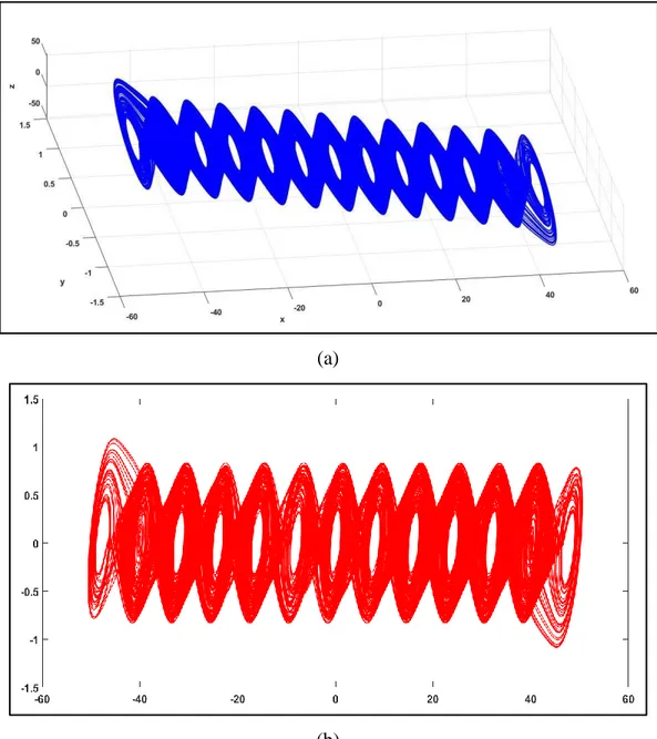
Figure 2.The 13-Spiral Attractor Generated by Equations (1) and (2) for 𝑐 = 12. (a) 3-Dimensional Figure, (b) Projection onto the Plane (x, y).
5 In order to compare the new integration duration based method versus the method previously introduced by Menacer et al.[27] we need a benchmark sequence of hidden bifurcations. In this goal, we limit our study to the case where parameter c is set to the value 12 which gives a 13 spirals attractor (Figure 2). This number of scrolls is enough to obtain a significant comparison. For a complete study of this model, with other values of c see Ref. [27].
THE MLC METHOD FOR METHOD FOR UNCOVERING HIDDEN
BIFURCATIONS
In the modified Chua circuit with sine function (1)–(2), the parameter c governing the number of spirals is an integer; hence, it is not possible to vary it continuously and therefore it is not possible to observe bifurcations of attractors from n to n + 2 spirals when the parameter c changes. Moreover, it is not possible to use non-integer real values for c. To overcome this obstacle, [27] introduced a new method for uncovering hidden bifurcations based on the core idea of the Leonov and Kuznetsov for searching hidden attractors (i.e. homotopy and numerical continuation, see Appendix). While keeping c constant, a new bifurcation parameter ε is introduced. We recall briefly this method in this section in which the value of parameters is fixed at 𝛼 = 11, 𝛽 = 15, 𝑎 = 2, 𝑏 = 0.2, 𝑐 = 12, 𝑑 = 𝜋.
The Method
For this purpose, we rewrite System (1)–(2) in the form Lur’e’s form [29]
𝑑𝑋 𝑑𝑡 = 𝑀𝑋 + 𝑞𝐻(𝑟 𝑇𝑋) 𝑋 ∈ 𝑅3, (5) where 𝑀 = ( 0 𝛼 0 1 −1 1 0 −𝛽 0 ) , 𝑋 = ( 𝑥 𝑦 𝑧 ) , 𝑞 = ( −𝛼 0 0 ) , 𝑟 = ( 1 0 0 ), and 𝐻(𝜎) = 𝑓(𝜎).
We introduce a coefficient and a small parameter in order to transform System (5) into the form similar to the system (V) as follows
0 3 0 ( ), T dX M X q g r X X R dt = + (6) where 𝑀0 = 𝑀 + 𝜒𝑞𝑟𝑇 = ( −𝛼𝜒 𝛼 0 1 −1 1 0 −𝛽 0 ), and 𝑔(𝜎) = 𝐻(𝜎) − 𝜒𝜎 = −𝛼𝑓(𝜎) − 𝜒𝜎.
Then considering the transfer function 𝑊(𝑚) (XI) solving the equations 𝐼𝑚 𝑊 (𝑖𝜔0) = 0and 𝜒 = − 𝑅𝑒 𝑊 (𝑖𝜔0)−1, which obtains 𝜔
6 By the non-singular linear transformation, 𝑋 = 𝑆𝑍 the System (6) is reduced to the form similar to Equation (VI)
𝑑𝑍 𝑑𝑡 = 𝐴𝑍 + 𝐵𝜀𝑔 0(𝐶𝑇𝑍), 𝑍 ∈ 𝑅3 (7) where 𝐴 = ( 0 −𝜔0 0 𝜔0 0 0 0 0 −𝑑1 ) , 𝑍 = ( 𝑧1 𝑧2 𝑧3) , 𝐵 = ( 𝑏1 𝑏2 1 ) , 𝐶 = ( 1 0 −ℎ ) . (8)
Remark: The System (1) being 3-dimensional, 𝑍3 of Equation (VI) is a scalar denoted here
𝑧3
This implies that
𝐴 = 𝑆−1𝑀0𝑆, 𝐵 = 𝑆−1𝑞, 𝐶𝑇 = 𝑟𝑇𝑆, and 𝑆 = (
𝑠11 𝑠12 𝑠13 𝑠21 𝑠22 𝑠23
𝑠31 𝑠32 𝑠33). (9)
The transfer function 𝑊𝐴(𝑚) of System (7) reads
𝑊𝐴(𝑚) =−𝑏1𝑚 + 𝑏2𝜔0 𝑚2+ 𝜔
02
+ ℎ
𝑚 + 𝑑1.
Then, using the equality of transfer of both functions 𝑊𝐴(𝑚) and
𝑊𝑀0(𝑚) = 𝑟𝑇(𝑀
0− 𝑚𝐼)−1𝑞 of Systems (6) and (7), we obtain the following relations
𝜒 =𝑎+𝜔02−𝛽 𝛼 , 𝑑1 = 𝛼 + 𝜔02− 𝛽 + 1, ℎ = 𝛼(𝛽 − 𝑑1+ 𝑑1 2) 𝜔02 + 𝑑 12 , 𝑏1 = 𝛼(𝛽 − 𝜔0 2− 𝑑 1) 𝜔02+ 𝑑12 , 𝑏2 =𝛼(1 − 𝑑1)(𝜔0− 𝛽𝑑1) 𝜔02(𝜔02+ 𝑑 12) . Numerical Example of Hidden Bifurcation Route
For the value of parameters fixed in this section, one obtains
𝜒 = 0.03796, 𝑑1 = 1.4176, ℎ = 26.686, 𝑏1 = 15.686, 𝑏2 = 3.1003,
And solving the matrix Equation (9) one gets 𝑆 = (
1 0 −26.686
0.03795 −0.19107 −2.4264
−1.3636 −0.27084 −25.674
).
Using Theorem 1 in the Appendix, for 𝜀 small enough, one obtains the following initial condition for the first step of the multi-stage localisation procedure:
7 𝑋0(0) = 𝑆𝑍(0) = 𝑆 ( 𝜏0 0 0 ) = ( 𝜏0𝑠11 𝜏0𝑠21 𝜏0𝑠31 ), (10)
Let us apply the localisation procedure described in the Appendix. First, we compute the starting frequency 𝜔0 and the coefficient of harmonic linearisation 𝜒 (already computed in
‘The method’ section). Using Equation (10), we obtain the initial conditions for the first step. Then, we compute the solutions of System (6) with the non-linearity 𝜀𝑔(𝑥) = 𝜀(𝐻(𝑥) − 𝜒𝑥), by increasing sequentially 𝜀 from the value 𝜀 = 0.1 to 𝜀 = 1 by starting at the beginning with the Step 0.1 and decreasing progressively it, down to 0.001 between 𝜀 = 0.8 and 𝜀 = 1.
If the stable periodic solution 𝑋1(𝑡) (corresponding to the small value 𝜀 = 0.1 near the harmonic one is determined, all the points of this stable periodic solution are located in the domain of attraction of the stable periodic solution 𝑋2(𝑡) of the system corresponding to 𝜀 = 0.2). The solution 𝑋2(𝑡) can be found numerically by searching one trajectory of System (5) with 𝜀 = 0.2 taking as an initial point 𝑋1(𝑡𝑚𝑎𝑥) where tmax is the last value of the integration
time. For the value of the parameter 𝜀 = 0.2 after a transient regime, the computational procedure reaches the periodic solution 𝑋2(𝑡). We continue by increasing the parameter using the same numerical procedure to obtain 𝑋3(𝑡), 𝑋4(𝑡), ⋯ , 𝑋𝑗(𝑡), ⋯ which are
solutions of Systems (1)–(2) for peculiar initial conditions. When 𝜀 = 0.8, the first chaotic solution possessing one scroll is found.
We apply the above procedure to obtain the initial conditions for the solutions for increasing values of 𝜀 as shown in Table 1.
Table 1. Initial Condition According to the Values of 𝜀
𝜺 𝑿𝒋(𝟎) 𝒙𝟎 𝒚𝟎 𝒛𝟎 0.1 𝑋1(0) = 𝑋0(𝑡 𝑚𝑎𝑥) 74.72 2.8356 −101.89 0.2 𝑋2(0) = 𝑋1(𝑡 𝑚𝑎𝑥) −3.5603 0.0978 5.1616 0.3 𝑋3(0) = 𝑋2(𝑡 𝑚𝑎𝑥) 3.7396 0.1166 −5.1258 0.4 𝑋4(0) = 𝑋3(𝑡 𝑚𝑎𝑥) 1.6312 0.7179 −1.3015 0.5 𝑋5(0) = 𝑋4(𝑡 𝑚𝑎𝑥) 2.9797 0.5334 −3.5896 0.6 𝑋6(0) = 𝑋5(𝑡 𝑚𝑎𝑥) 3.1137 −0.2868 −4.7176 0.7 𝑋7(0) = 𝑋6(𝑡 𝑚𝑎𝑥) −3.2894 −0.5358 3.9445 0.8 𝑋8(0) = 𝑋7(𝑡 𝑚𝑎𝑥) −3.5390 0.2601 4.9005 0.86 𝑋9(0) = 𝑋8(𝑡 𝑚𝑎𝑥) −3.5920 0.1733 5.0637 0.9785 𝑋10(0) = 𝑋9(𝑡 𝑚𝑎𝑥) 10.5751 0.1758 −11.8656 0.989 𝑋11(0) = 𝑋10(𝑡 𝑚𝑎𝑥) −12.1911 0.3828 11.2562 0.993 𝑋12(0) = 𝑋11(𝑡 𝑚𝑎𝑥) −7.4755 −0.6595 5.6561 0.9953 𝑋13(0) = 𝑋12(𝑡 𝑚𝑎𝑥) 8.9249 0.7895 −7.6282 0.9994 𝑋14(0) = 𝑋13(𝑡 𝑚𝑎𝑥) −2.8006 −0.2619 3.9268 1 𝑋15(0) = 𝑋14(𝑡𝑚𝑎𝑥) −2.6705 0.2845 2.2206
8 Using these initial conditions, we get the solutions 𝑋8(𝑡)
(Figure 3a) with one scroll to 𝑋14(𝑡) (Figure 5g). In each figure, there are a different odd number of spirals in the attractor. The number of spiral increases by 2 at each step as displayed in Table 2 from 1 to 13 spirals. The values of 𝜀 in this table are exactly the values of bifurcation points. In Figure 3, we display the hidden bifurcations of the multi-spiral Chua’s attractor.
Table 2. Values of Parameter 𝜀 at the Bifurcation Points for c = 12 (13 Spirals) 𝜺
0.80 0.86 0.9785 0.989 0.993 0.9953 0.9994
𝑋8(0) 𝑋9(0) 𝑋10(0) 𝑋11(0) 𝑋12(0) 𝑋13(0) 𝑋14(0) 1 spiral 3 spirals 5 spirals 7 spirals 9 spirals 11 spirals 13 spirals
9 Figure 3. (Continued)
10 Figure 3. The Increasing Number of Spirals of System (6) According to Increasing ε Values. (a) 1-Spiral for ε =
0.80, (b) 3-Spirals for ε=0.86, (c) 5-Spirals for ε=0.9785, (d) 7-Spirals for ε=0.989, (e) 9-Spirals for ε=0.993, (f) 11-Spirals for ε=0.9953, (g) 13-Spirals for ε=0.9994
INTEGRATION DURATION METHOD FOR UNVEILING HIDDEN
PATTERNS OF EVEN NUMBER OF SPIRALS
In the previous section, it is shown that the attractors along the hidden bifurcation route display an odd number of spirals. In this section, we introduce a novel method for unveiling hidden patterns of even number of spirals. This method based on the duration of integration of Systems (1)–(2). For this novel method, we fix ε and we increase the duration of integration tmax. During the integration process, before reaching the asymptotical attractor which
possesses and odd the number of spirals, the number of spirals increases until it reaches the maximum number corresponding to the value fixed by ε.
As a numerical example, we set the value of ε to 0.9953. For this value, 11 spirals belong to the asymptotic attractor (Figure3f). All the patterns are displayed in Figure 4 and the value of tstepmax is given in Table 3. In each figure, the number of spiral increases by 1 (instead of 2
in the MLC method). The MATLAB’s standard solver for ordinary differential equations ode45 is used in order to integrate the Chua’s system. This function implements a Runge–
11 Kutta method with a variable time step. Therefore, it is difficult to know tmax. The value tstepmax
(shown in Table 3) which is the maximum number of steps used (i.e. corresponding to the duration of integration).
Table 3. Values of tstepmax for = 0.9953 and c= 12
tstepmax 144 2050 2070 2700 6090 6700 Number of spirals 1 2 3 4 5 6 Figure 4a 4b 4c 4d 4e 4f tstepmax 9590 14,000 70,000 88,210 200,000 Number of spirals 7 8 9 10 11 Figure 4g 4h 4i 4j 4k Figure 4. (Continued)
12 Figure 4. (Continued)
13 Figure 4. (Continued)
14 Figure 4. (Continued)
15 Figure 4. The Increasing Number of Spirals for the Same Values of ε = 0.9953 and Various Values of tstepmax. (a)
1-Spirals for tstepmax = 144, (b) 2-Spirals for tstepmax = 2050, (c) 3-Spirals for tstepmax = 2070, (d) 4-Spirals for tstepmax
= 2700, (e) 5-Spirals for tstepmax = 6090, (f) 6-Spirals for tstepmax = 6700, (g) 7-Spirals for tstepmax = 9590, (h)
8-Spirals for tstepmax = 4000, (i) 9-Spirals for tstepmax = 70,000, (j) 10-Spirals for tstepmax = 88,210, (k) 11-Spirals for
tstepmax = 200,000
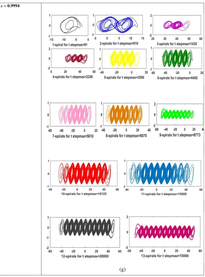
In order to highlight the efficiency of this integration duration based method, we repeat the same procedure for all values of ε of Table 2, we are going to observe the change of scroll number and we resume our results in Table 4 and Figure 5.
16 Table 4. Values of tstepmax for 𝜀 = 0.80 to 𝜀 = 0.9994 and c = 12
ε = 0.80 tstepmax 50,000 Nb of spirals 1 ε = 0.86 tstepmax 7200 19,000 41,430 Nb of spirals 1 2 3 ε = 0.97885 tstepmax 195 680 20,000 90,000 100,000 Nb of spirals 1 2 3 4 5 ε = 0.989 tstepmax 95 350 1000 1380 6000 Nb of spirals 1 2 3 4 5 tstepmax 80,000 90,110 Nb of spirals 6 7 ε = 0.993 tstepmax 85 2260 2300 2340 9310 Nb of spirals 1 2 3 4 5 tstepmax 9410 36,090 36,322 90,000 Nb of spirals 6 7 8 9 ε = 0.9953 tstepmax 144 2050 2070 2700 6090 Nb of spirals 1 2 3 4 5 tstepmax 6700 9590 14,000 60,000 88,210 Nb of spirals 6 7 8 9 10 tstepmax 200,000 Nb of spirals 11 ε = 0.9994 tstepmax 91 910 1435 2250 3590 Nb of spirals 1 2 3 4 5 tstepmax 4450 5610 8070 8773 10,125 Nb of spirals 6 7 8 9 10 tstepmax 15,000 20,000 70,000 Nb of spirals 11 12 13
17
Values of ε Number of spirals
ε = 0.80
(a)
ε = 0.86
18 ε = 0.97885
(c) ε = 0.989
19 ε = 0.993
20 ε = 0.9953
21 ε = 0.9994
(g)
22
CONCLUSION
In this article, we have introduced a novel method for unveiling hidden patterns of even number of spirals in the multi-spiral Chua Chaotic attractor. This method is based on the duration of integration of this system and allows displaying every pattern containing from 1 to c + 1 spirals of this attractor. After having given the equation of the multi-spiral Chua Chaotic attractor, the MLC method for uncovering hidden bifurcations is explained again and a numerical example of a route of bifurcation is given. In the chosen example, it is shown that the attractors found along this hidden bifurcation route display an odd number of spirals. With the novel method, during the integration process, before reaching the asymptotical attractor which possesses and odd the number of spirals, the number of spirals increases one by one until it reach the maximum number corresponding to the value fixed by ε, unveiling both patterns of even and odd number of spirals.
APPENDIX
ANALYTICAL-NUMERICAL METHOD FOR HIDDEN ATTRACTOR
LOCALISATION
Ten years ago, Kuznetsov and Leonov[25, 26] proposed an effective method for the numerical localisation of hidden attractors in multi-dimensional dynamical systems.
Their method is based on homotopy and numerical continuation. They construct a sequence of similar systems such that for the first (starting) system the initial data for numerical computation of an oscillating solution (starting oscillation) can be obtained analytically. Then the transformation of this starting solution is tracked numerically in passing from one system to another. This proposed approach is generalised in the work [23] to the systems of the form
𝑑𝑋
𝑑𝑡 = 𝑀𝑋 + 𝐻̱(𝑋) (I)
where 𝑀 is a constant 𝑛 × 𝑛 matrix, 𝐻̱(𝑋) is a continuous vector-function and 𝐻̱(0) = 0. They consider a system having one scalar non-linearity, which takes the following form:
𝑑𝑋
𝑑𝑡 = 𝑀𝑋 + 𝑞𝐻(𝑟
𝑇𝑋), 𝑋 ∈ ℝ𝑛 (II)
Here 𝑞, 𝑟 are constant n-dimensional vectors, T is the transposition operation, 𝐻(𝜎) is a
continuous piecewise differentiable scalar function satisfying the condition 𝐻(0) = 0. They then define a coefficient of harmonic linearisation 𝜒 in such a way that the matrix
𝑀0 = 𝑀 + 𝜒𝑞𝑟𝑇 (III)
has a pair of purely imaginary eigenvalues ±𝜔0 , (𝜔0 > 0) and the rest of its eigenvalues have negative real parts. They assume that such 𝜒 exists and they can rewrite the System (II) as
𝑑𝑋
𝑑𝑡 = 𝑀0𝑋 + 𝑞𝑔(𝑟
23 where 𝑔(𝜏) = 𝐻(𝜏) − 𝜒𝜏.
After that, they introduce a finite sequence of functions 𝑔0(𝜏), 𝑔1(𝜏), … , 𝑔𝑚(𝜏) such that the graph of the functions 𝑔𝑗(𝜏) and 𝑔𝑗+1(𝜏), (𝑗 = 0, … , 𝑚 − 1) differs slightly from one to another, where the function 𝑔0(𝜏) is the small and 𝑔𝑚(𝜏) = 𝑔(𝜏). Using the smallness of
function, they can apply the method of harmonic linearisation (describing function method) for the system
𝑑𝑋
𝑑𝑡 = 𝑀0𝑋 + 𝑞𝑔
0(𝑟𝑇𝑋) (V)
in order to determine the non-trivial stable periodic solution 𝑋0(𝑡). For the localisation of the
attractor of the original System (IV), they follow numerically the transformation of this periodic solution (a starting oscillating attractor, not including equilibria, denoted further by 𝐴0 with increasing j).
To determine the initial condition 𝑋0(0) of the periodic solution, the System (V) can be transformed by a linear non-singular transformation S (X = SZ) to the form
{ 𝑧̇1(𝑡) = − 𝜔0𝑧2(𝑡) + 𝑏1𝑔0(𝑧1(𝑡) + 𝑐3𝑇𝑍3(𝑡)) 𝑧̇2(𝑡) = 𝜔0𝑧1(𝑡) + 𝑏2𝑔0(𝑧 1(𝑡) + 𝑐3𝑇𝑍3(𝑡)) 𝑍̇3(𝑡) = 𝐴3𝑍3(𝑡) + 𝐵3𝑔0(𝑧1(𝑡) + 𝑐3𝑇𝑍3(𝑡)) (VI)
Here, 𝑧1(𝑡), 𝑧2(𝑡) are scalar values, 𝑍3(𝑡) is a(𝑛 − 2) dimensional vector; 𝐵3 and 𝑐3 are
(𝑛 − 2) dimensional vectors, 𝑏1 and𝑏2 are real numbers; 𝐴3 is (𝑛 − 2) × (𝑛 − 2) matrix, whose all of its eigenvalues have negative real parts. Without loss of generality, it can be assumed that for the matrix 𝐴3 there exists a positive number 𝑑1 > 0 such that
𝑍3𝑇(𝑡)(𝐴3+ 𝐴3𝑇)𝐴𝑍3(𝑡) ≤ −2𝑑1|(𝑍3(𝑡))2|, ∀𝑍3 ∈ 𝑅𝑛−2, (VII)
In the scalar case, they define the following describing function 𝐺 of a real variable 𝜏 and assume the existence of its derivative:
𝐺(𝜏) = ∫ 𝑔(𝑐𝑜𝑠( 𝜔0𝑡)𝜏) 𝑐𝑜𝑠( 𝜔0𝑡)𝑑𝑡
2𝜋 𝜔0
0 (VIII)
Theorem 1 [25] If it can found a positive 𝜏0such that
𝐺(𝜏0) = 0, 𝑏1𝑑𝐺(𝜏)
𝑑𝜏 |𝜏=𝜏0 < 0 (IX)
then for the initial condition of the periodic solution 𝑋0(0) = 𝑆(𝑧1(0), 𝑧2(0), 𝑍3(0))𝑇. At the initial step of the algorithm, one has 𝑧1(0) = 𝜏0+ 𝑂(𝜀), 𝑧2(0) = 0, 𝑍3(0) = 𝑂𝑛−2(𝜀), where 𝑂𝑛−2(𝜀) is an (𝑛 − 2) dimensional vector such that all its components are 𝑂(𝜀).
For the stability of 𝑋0(𝑡) (where stability is defined in the sense that for all solutions with
the initial data sufficiently close to 𝑋0(0) the modulus of their difference with 𝑋0(𝑡) is uniformly bounded for all 𝑡 > 0), it is sufficient to require the following condition is true:
24 𝑏1
𝑑𝐺(𝜏)
𝑑𝜏 |𝜏=𝜏0 < 0 (X)
In practice, to determine 𝜒 and 𝜔0
, one uses the transfer function 𝑊(𝑚) of the System (IV)
𝑊(𝑚) = 𝑟(𝑀 − 𝑚𝐼)−1𝑞 (XI)
where m is a complex variable. The number 𝜔0 is determined from the equation
𝐼𝑚 𝑊 (𝑖𝜔0) = 0 and 𝜒 is calculated then by the formula 𝜒 = − 𝑅𝑒 𝑊 (𝑖𝜔0)−1.
REFERENCES
[1] Poincaré H. 1885. L'Équilibre d'une masse fluide animée d'un mouvement de rotation. Acta
Mathematica, 7(1), pp. 259–380.
[2] Sattinger DH, 1973. Topics in stability and bifurcation theory, Lecture Notes in math, Springer-Verlag, Berlin/New York, p. 309.
[3] Lozi R, 1975. A computing method for bifurcation boughs of nonlinear eigen value problems. Bulletin of
the American Mathematical Society, 81(6), pp. 1127–1129.
[4] Marsden JE, McCracken M, 1976. The Hopf bifurcation and its applications. Applied Mathematical
Sciences, 19, p. 424.
[5] Lorenz E, 1963. Deterministic non-periodic flow. Journal of Atmospheric Science, 20(2), p. 130–141. [6] Chua LO, 1992. The genesis of Chua’s circuit. Archiv 𝑓𝑢̈𝑟 Elektronik und Ubertragung-stechnik, 46, pp.
250–257.
[7] Duan Z, Wang J, Huang L, 2004. Multiinput and multi-output nonlinear systems interconnected Chua’s circuits. International Journal of Bifurcation and Chaos, 14(3), pp. 3065–3081.
[8] Zhong GQ, Ayrom F, 1985. Experimental confirmation of chaos from Chua’s circuit. International
Journal of Circuit Theory and Applications, 13, pp. 93–98.
[9] Matsumoto T, 1984. A chaotic attractor from Chua’s Circuit. IEEE Transaction on Circuits and Systems, 31, pp. 1055–1558.
[10] Chua LO, Komuro M, Matsumoto T, 1986. The double scroll family. IEEE Transactions on Circuits
and Systems, 33, pp. 1072–1118.
[11] Lozi R, Ushiki S, 1993. The theory of confinors in Chua’s circuit: accurate analysis of bifurcations and attractors. International Journal of Bifurcation and Chaos, 3(2), pp. 333–361.
[12] Boughaba S, Lozi R, 2000. Fitting trapping regions for Chua’s attractor—a novel method based on isochronic lines. International Journal of Bifurcation and Chaos, 10(1), pp. 205–225.
[13] Khibnik AI, Roose D, Chua LO, 1993. On periodic orbits and homoclinic bifurcations in Chua’s circuit with a smooth nonlinearity. International Journal of Bifurcation and Chaos, 3, pp. 363–384.
[14] Shilnikov LP, 1994. Chua’s circuit: rigorous results and future problems. International Journal of
Bifurcation and Chaos, 4, pp. 489–519.
[15] Huang AS, Pivka L, Wu CW, Franz M, 1996. Chua’s equation with cubic nonlinearity. International
Journal of Bifurcation and Chaos, 12A, pp. 2175–2222.
[16] Hirsch MW, Smale S, Devaney RL, 2003. Differential equations, dynamical systems and an
introduction to chaos. Second edition. Elsevier, Academic Press, Amsterdam.
[17] Suykens JAK, Vandewalle J, 1991. Quasilinear approach to nonlinear systems and the design of n-double scroll (n = 1; 2; 3; 4; . . .). Proceedings of the IEEE. Institute of Electrical and Electronics
Engineers, 138(5), pp. 595–603.
[18] Arena P, Baglio S, Fortuna L, Manganaro G, 1996. Generation of n-double scrolls via cellular neural networks. International Journal of Circuit Theory and Applications, 24(3), pp. 241–252.
[19] Suykens JAK, Huang A, Chua LO, 1997. A family of n-scroll attractors from a generalized Chua’s circuit. International Journal of Electronics and Communications, 51(3), pp. 131–138.
[20] Yalçin ME, Suykens JAK, Vandewalle J, 2000. Experimental confirmation of 3-and 5-scroll theory attractors from a generalized Chua’s circuit. IEEE Transaction on Circuits and Systems-Part I
25
[21] Tang KS, Zhong GQ, Chen G, Man KF, 2001. Generation of n-scroll attractors via sine function. IEEE
Transactions on Circuits and Systems, 48(11), pp. 1369–1372.
[22] Leonov GA, Kuznetsov NV, Vagaitsev VI, 2011. Localization of hidden Chua’s attractors. Physics
Letters A, 375, pp. 2230–2233.
[23] Leonov GA, Kuznetsov NV, 2011. Analytical-numerical methods for investigation of hidden
oscillations in nonlinear control systems. Preprints of the 18th IFAC World Congress, Milano, Italy, 2,
pp. 2494–2505.
[24] Leonov GA, 2009. On harmonic linearization method. Automation and Remote Control, 5, pp. 65–75. [25] Leonov GA, Vagaitsev VI, Kuznetsov NV, 2010. Algorithm for localizing Chua attractors based on the
harmonic linearization method. Doklady Mathematics D, 82, pp. 663–666.
[26] Leonov GA, Kuznetsov NV, Vagaitsev VI, 2012. Hidden attractor in smooth Chua systems. Physica D, 241, pp. 1482–1486.
[27] Menacer T, Lozi R, Chua L, 2016. Hidden bifurcations in the multispiral Chua attractor. International
Journal of Bifurcation and Chaos, 26(14), p. 1630039 (26 pages).
[28] Madan RN, editor, 1993. Chua’s circuit: a paradigm for chaos. World Scientific Series on Nonlinear
Science Series B, 1, p. 1043.
[29] Lur’e AI, 1951. Certain nonlinear problems in the theory of automatic control. Gostekhizat, Moscow, Leningrad. Translated into English, H.M. Stationery, 1957.