HAL Id: hal-01166275
https://hal.archives-ouvertes.fr/hal-01166275
Submitted on 22 Jun 2015
HAL is a multi-disciplinary open access
archive for the deposit and dissemination of
sci-entific research documents, whether they are
pub-lished or not. The documents may come from
teaching and research institutions in France or
abroad, or from public or private research centers.
L’archive ouverte pluridisciplinaire HAL, est
destinée au dépôt et à la diffusion de documents
scientifiques de niveau recherche, publiés ou non,
émanant des établissements d’enseignement et de
recherche français ou étrangers, des laboratoires
publics ou privés.
Discussion of ”Revisiting the Energy-Momentum
Method for Rating Vertical Sluice Gates under
Submerged Flow Conditions” by Oscar Castro-Orgaz,
Luciano Mateos, and Subhasish Dey
Gilles Belaud, Ludovic Cassan, Jean-Pierre Baume
To cite this version:
Gilles Belaud, Ludovic Cassan, Jean-Pierre Baume. Discussion of ”Revisiting the Energy-Momentum
Method for Rating Vertical Sluice Gates under Submerged Flow Conditions” by Oscar Castro-Orgaz,
Luciano Mateos, and Subhasish Dey. Journal of Irrigation and Drainage Engineering, American
Society of Civil Engineers, 2014, vol. 140 (n° 7), pp. 1-3. �10.1061/(asce)ir.1943-4774.0000691�.
�hal-01166275�
Open Archive TOULOUSE Archive Ouverte (OATAO)
OATAO is an open access repository that collects the work of Toulouse researchers and
makes it freely available over the web where possible.
This is an author-deposited version published in :
http://oatao.univ-toulouse.fr/
Eprints ID : 13862
To cite this version : Belaud, G. and Cassan, L. and Baume, J.
Discussion of "Revisiting the Energy-Momentum Method for Rating
Vertical Sluice Gates under Submerged Flow Conditions" by Oscar
Castro-Orgaz, Luciano Mateos, and Subhasish Dey. (2014) Journal of
Irrigation and Drainage Engineering, vol. 140 (n° 7). pp. 1-3. ISSN
0733-9437
To link to this article :
DOI: 10.1061/(ASCE)IR.1943-4774.0000691
URL:
http://dx.doi.org/10.1061/(ASCE)IR.1943-4774.0000691
Discussion of
“Revisiting the
Energy-Momentum Method for Rating Vertical Sluice
Gates under Submerged Flow Conditions”
by Oscar Castro-Orgaz, Luciano Mateos, and
Subhasish Dey
G. Belaud1; L. Cassan2; and J.-P. Baume3
1Professor, Unité Mixte de Recherche G-eau, Montpellier Supagro, 2 place
P. Viala, 34060 Montpellier cedex 1, France (corresponding author). E-mail: belaud@supagro.inra.fr
2Assistant Professor, Institut de Mécanique des Fluides, Toulouse, allée
prof. Camille Soula, 31400 Toulouse, France. E-mail: lcassan@imft.fr
3Senior Hydraulic Engineer, Unité Mixte de Recherche G-eau, Irstea,
BP 5095, 34196 Montpellier cedex 5, France. E-mail: jean-pierre .baume@irstea.fr
The discussers really appreciated the efforts to make more solid some usual assumptions used to derive reliable stage-discharge relationships, and the confrontation with field measurements. Energy and momentum equations are generally applied in their standard form, as presented in most hydraulic engineering books. The authors are right to point out that some of these assumptions are simplistic, which introduces biases in the derived relationships. Velocity distribution is one of these assumptions, and trying to im-prove this distribution is commendable. Head loss is another crucial issue, especially for submerged gates where the presence of the roller above the jet induced large dissipation. The authors also ne-glected the friction forces and assumed that contraction coefficient (Cc) is the same in submerged flow as in free flow. This assumption
was questioned by Henderson (1989), and Belaud et al. (2009)
showed how to derive a continuous relationship for Cc between
low submergence (Cc about 0.61) and fully open gate (Cc¼ 1). For submerged gates, there have been a limited number of exper-imental studies that explored the validity of the most sensitive as-sumptions. Compared to free flow, much more phenomena need to be quantified, such as head loss due to jet–roller interaction, veloc-ity distributions at the contracted section and downstream measur-ing section, friction forces between these two sections. The effect of submergence introduces another dimension when trying to elabo-rate generic relationships. As the practical objectives are to obtain accurate discharge predictions, a common approach is to calibrate corrections using measured discharges, water levels, and openings. This may not be sufficient to validate physically based improve-ments since several phenomena compensate for each other.
The pioneer experimental works used by the authors provided very useful data sets to perform this analysis. This discussion is based on recent experimental and numerical results presented by
Cassan and Belaud (2012). Experiments used acoustic Doppler
velocimetry at selected locations, for three configurations in free flow and three in submerged flow. Computational fluid dynamics was used in complement, with the objective to interpolate flow characteristics between measuring points and to explore other configurations than those measured. Experiments were essential to verify the validity of the numerical results, based on Reynolds–
Average Navier–Stokes simulations with the volume-of-fluid
method and Reynolds stress model as turbulence closure model. Notations are those of the discussed paper.
Velocity Distribution
One usual assumption is that the fluxes of energy and momentum in the roller are negligible. With an improved velocity profile, such
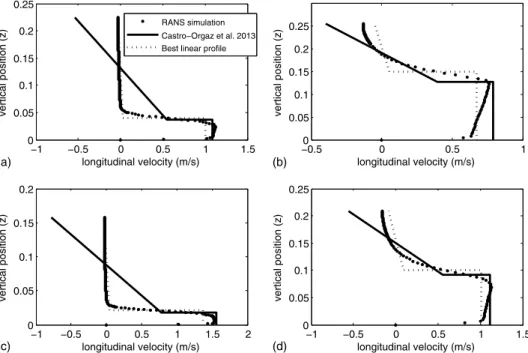
−1 −0.5 0 0.5 1 1.5 0 (a) (b) (c) (d) 0.05 0.1 0.15 0.2 0.25 longitudinal velocity (m/s) vertical position (z) RANS simulation Castro−Orgaz et al. 2013 Best linear profile
−0.50 0 0.5 1 0.05 0.1 0.15 0.2 0.25 longitudinal velocity (m/s) vertical position (z) −1 −0.5 0 0.5 1 1.5 2 0 0.05 0.1 0.15 0.2 longitudinal velocity (m/s) vertical position (z) −1 −0.5 0 0.5 1 1.5 0 0.05 0.1 0.15 0.2 0.25 longitudinal velocity (m/s) vertical position (z)
Fig. 1. Velocity profiles for various simulated configurations (selection of four typical configurations; other results are available on request); Vj is
as the one proposed in the paper under discussion, these fluxes can be quantified. It further allows estimating a head loss coefficient [Eqs. (22) and (23)]. Considering a calibration on Boussinesq co-efficients, the authors obtainUr=Vj¼ 0.5. This results in a correct fitting for some configurations, but not all. Fig. 1 presents the velocity profiles obtained at the contracted section (Section 2, see Fig. 1 of discussed paper), defined as the one where the jet thickness is minimum. For most flow conditions, it can be observed that Ur=Vj should be closer to 0 than to 0.5, which means that the configuration of Fig.2(b) of the authors better describes the
velocity distribution than the one of Fig. 2(c). The data set used
in this discussion may be useful to find a relation between Ur
and Vj. RANS simulations indicate some dependency between
Ur=Vj, obtained by a least square error fitting method on the veloc-ity profiles, and relative submergence (Fig.2). As expected, when the column of water above the jet is large,Urmust tend to a very small proportion of the jet velocity, about 2% for experiment S 01. The fact that it better fits the relationship betweenβ and y=h may be due to the experimental points considered by the authors in their analysis. They used indeed several points along the jet, whereas Fig.1above is only for Section 2. After mixing, the veloc-ity profiles tend to uniformveloc-ity, which explains why Ur=Vj
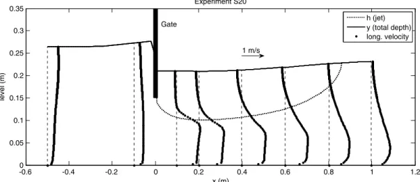
in-creases. As an example, Fig. 3 presents the velocity profiles
along the jet for simulation S20. While Ur=Vj is close to zero at Section 2, it regularly increases along the jet to reach the value of 1 far behind the roller. The value 0.5 is acceptable in average. Fig.4shows the values ofβ calculated in the jet. Fig.4(a)uses all the calculated locations within the jet, and corresponds to Fig.3(a)
of the authors. Values of β are above the line β ¼ y=h, and the
highest values ofβ=ðy=hÞ are rather well described by Eq. (14)
of the authors. However, the momentum equation (Eq. 3) should not use all these values but only the ones at Sections 2 and 3. In particular, the values ofβ2 [Fig.4(b)] do not present the same spreading as in Fig.4(a)of this discussion or Fig.3of the authors.
The best fitting gives β2≈ 1.064y2=h2. Using the velocity
distribution of the authors, this in turn gives
0.10 0.09 0.08 0.07 0.06 0.05 0.04 0.03 0.02 0.01 0.00 0 5 10 15 submergence rate (y2-h2)/h2 Ur /Vj
Fig. 2. Fitted values of Ur=Vj, as a function of submergence rate ðy2− h2Þ=h2 -0.60 -0.4 -0.2 0 0.2 0.4 0.6 0.8 1 1.2 0.05 0.1 0.15 0.2 0.25 0.3 0.35 Experiment S20 x (m) level (m) h (jet) y (total depth) long. velocity Gate 1 m/s
Fig. 3. Longitudinal velocity profiles at different locations, upstream and downstream of the gate
0 5 10 15 0 5 10 15 B o u ssi ne sq co effi ci ent β y/h β at section 2 β=1.064 y/h (r²=0.9998) (a) (b)
Ur Vj ¼ ffiffiffiffiffiffiffiffiffiffiffiffiffiffiffiffiffiffiffi 30.064hy 2 2− h2 s
with the asymptotic trend observed in Fig. 2, although it yields larger values than those obtained by fitting on velocity profiles. This suggests considering more complex velocity distributions.
Revisiting Pressure Distribution, Contraction, and Friction
Friction introduces head loss in the energy equation, as well as a friction force in the momentum equation. This force was not con-sidered by the authors, as it is assumed to be counterbalanced by other effects. The discussers appreciate the link made between velocity distribution and head loss [Eqs. (22) and (23)]. There is no clear conclusion about the prediction of head loss coefficients, as the calibrated values depend on the underlying assumptions (regarding pressure and velocity distributions, friction force), but the approach is an encouragement to continue the efforts for improving physically based relationships. Among these
assump-tions, Rajaratnam and Subramanya (1967) showed that pressure
is not perfectly hydrostatic at the vena contracta, and that the
ratio λ of bottom pressure head deviation to the kinetic energy
was between 0.05 and 0.08, which is consistent with the
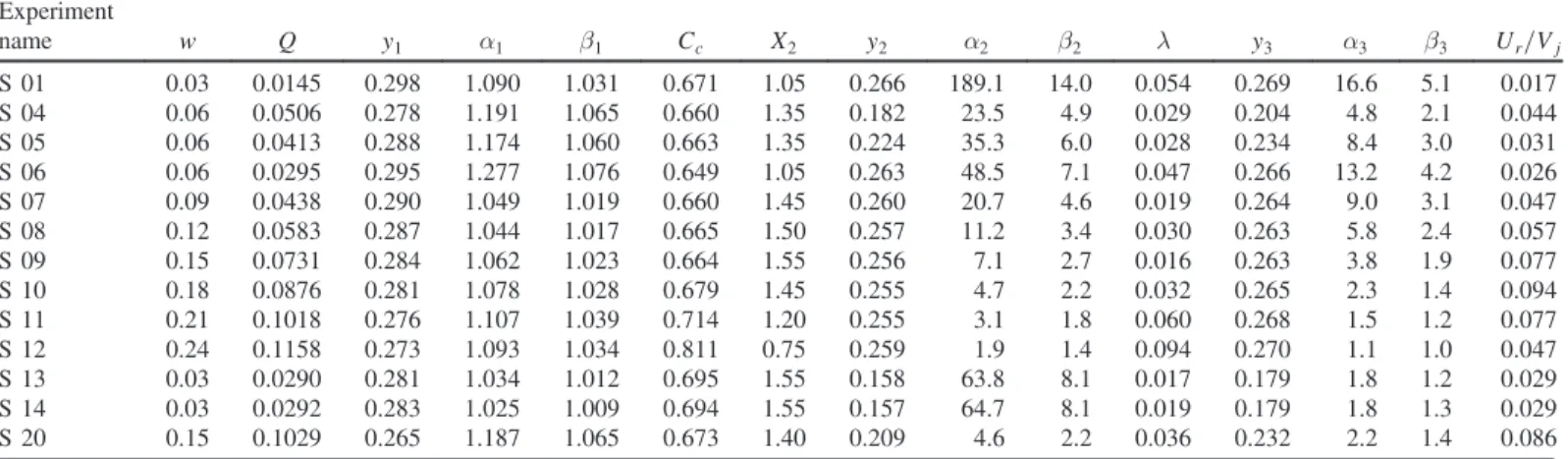
simulations used in this discussion (Table1, Fig.5). This effect is
somewhat counterbalanced in the momentum–energy system of
equations (Belaud et al. 2009), and the residual effect can be added to energy loss.
Contraction coefficient is another issue, particularly in sub-merged flow as it is not directly observed from the water profile. Experiments and simulation results show that the position of the vena contracta (x2) is betweenw and 1.5w downstream of the gate. The results also show that Cc significantly deviates from 0.61, particularly at large openings in submerged flows. However, as considered by the authors,Cccan be considered as constant until a ≈ 0.6, but then it largely increases to reach unity as the gate be-comes fully open (Table1). As pointed out by the authors, taking Ccas a constant while calibrating the discharge equation on exper-imental data can be counterbalanced by other simplifying assump-tions or by changing other coefficients, like velocity, pressure, or friction coefficients. This means that the energy-momentum (EM) method, although it may appear as physically based, remains an empirical method, so fitted relationships may not apply universally. Despite its complexity, it is still a promising method that can deal with particular gate configurations and flow regimes (like transi-tions from free to submerged flow or from gate to weir flow) frequently observed in irrigation systems. Further works should quantify the various effects, and lead to generic relationships that could be included in the EM method.
References
Belaud, G., Cassan, L., and Baume, J.-P. (2009).“Calculation of contrac-tion coefficient under sluice gates and applicacontrac-tion to discharge meas-urement.”J. Hydraul. Eng., 10.1061/(ASCE)HY.1943-7900.0000122, 1086–1091.
Cassan, L., and Belaud, G. (2012). “Experimental and numerical studies of the flow structure generated by a submerged sluice gate.” J. Hydraul. Eng., 10.1061/(ASCE)HY.1943-7900.0000514, 367–373.
Henderson, F. M. (1989). Open channel flow, MacMillan Publishing, New York.
Rajaratnam, N., and Subramanya, K. (1967).“Flow immediately below submerged sluice gate.” J. Hydr. Div. ASCE, 93(4), 57–77.
0 0.01 0.02 0.03 0.04 0.05 0.06 0.07 0.08 0.09 0.1 0.0 0.2 0.4 0.6 0.8 1.0 pressure coefficient relative opening
Fig. 5. Pressure correction coefficient
Table 1. Calculated Variables for Selected Numerical Experiments in Submerged Flow Experiment name w Q y1 α1 β1 Cc X2 y2 α2 β2 λ y3 α3 β3 Ur=Vj S 01 0.03 0.0145 0.298 1.090 1.031 0.671 1.05 0.266 189.1 14.0 0.054 0.269 16.6 5.1 0.017 S 04 0.06 0.0506 0.278 1.191 1.065 0.660 1.35 0.182 23.5 4.9 0.029 0.204 4.8 2.1 0.044 S 05 0.06 0.0413 0.288 1.174 1.060 0.663 1.35 0.224 35.3 6.0 0.028 0.234 8.4 3.0 0.031 S 06 0.06 0.0295 0.295 1.277 1.076 0.649 1.05 0.263 48.5 7.1 0.047 0.266 13.2 4.2 0.026 S 07 0.09 0.0438 0.290 1.049 1.019 0.660 1.45 0.260 20.7 4.6 0.019 0.264 9.0 3.1 0.047 S 08 0.12 0.0583 0.287 1.044 1.017 0.665 1.50 0.257 11.2 3.4 0.030 0.263 5.8 2.4 0.057 S 09 0.15 0.0731 0.284 1.062 1.023 0.664 1.55 0.256 7.1 2.7 0.016 0.263 3.8 1.9 0.077 S 10 0.18 0.0876 0.281 1.078 1.028 0.679 1.45 0.255 4.7 2.2 0.032 0.265 2.3 1.4 0.094 S 11 0.21 0.1018 0.276 1.107 1.039 0.714 1.20 0.255 3.1 1.8 0.060 0.268 1.5 1.2 0.077 S 12 0.24 0.1158 0.273 1.093 1.034 0.811 0.75 0.259 1.9 1.4 0.094 0.270 1.1 1.0 0.047 S 13 0.03 0.0290 0.281 1.034 1.012 0.695 1.55 0.158 63.8 8.1 0.017 0.179 1.8 1.2 0.029 S 14 0.03 0.0292 0.283 1.025 1.009 0.694 1.55 0.157 64.7 8.1 0.019 0.179 1.8 1.3 0.029 S 20 0.15 0.1029 0.265 1.187 1.065 0.673 1.40 0.209 4.6 2.2 0.036 0.232 2.2 1.4 0.086 Note:Q Discharge (m3=s); X2¼ x2=w relative position of vena contracta. Dimensional variables are in SI units.