HAL Id: lirmm-01348420
https://hal-lirmm.ccsd.cnrs.fr/lirmm-01348420
Submitted on 18 Dec 2019
HAL is a multi-disciplinary open access
archive for the deposit and dissemination of
sci-entific research documents, whether they are
pub-lished or not. The documents may come from
teaching and research institutions in France or
abroad, or from public or private research centers.
L’archive ouverte pluridisciplinaire HAL, est
destinée au dépôt et à la diffusion de documents
scientifiques de niveau recherche, publiés ou non,
émanant des établissements d’enseignement et de
recherche français ou étrangers, des laboratoires
publics ou privés.
On the fixed parameter tractability of agreement-based
phylogenetic distances
Magnus Bordewich, Celine Scornavacca, Nihan Tokac, Mathias Weller
To cite this version:
Magnus Bordewich, Celine Scornavacca, Nihan Tokac, Mathias Weller. On the fixed parameter
tractability of agreement-based phylogenetic distances. Journal of Mathematical Biology, Springer
Verlag (Germany), 2017, 74 (1-2), pp.239-257. �10.1007/s00285-016-1023-3�. �lirmm-01348420�
On
the Fixed Parameter Tractability of
Agreement-based
Phylogenetic Distances
Magnus Bordewich, Celine Scornavacca, Nihan Tokac and Mathias Weller
Abstract Three important and related measures for summarizing the dissim-ilarity in phylogenetic trees are the minimum number of hybridization events required to fit two phylogenetic trees onto a single phylogenetic network (the hybridization number), the (rooted) subtree prune and regraft distance (the rSPR distance) and the tree bisection and reconnection distance (the TBR dis-tance) between two phylogenetic trees. The respective problems of computing these measures are known to be NP-hard, but also fixed-parameter tractable in their respective natural parameters. This means that, while they are hard to compute in general, for cases in which a parameter (here the hybridiza-tion number and rSPR/TBR distance, respectively) is small, the problem can be solved efficiently even for large input trees. Here, we present new analy-ses showing that the use of the “cluster reduction” rule – already defined for the hybridization number and the rSPR distance and introduced here for the TBR distance – can transform any O(f(p) · n)-time algorithm for any of these problems into an O(f(k) · n)-time one, where n is the number of leaves of the phylogenetic trees, p is the natural parameter and k is a much stronger (that
Magnus Bordewich
School of Engineering and Computing Sciences, Durham University, Durham DH1 3LE, U.K., E-mail: [email protected]
Celine Scornavacca
Institut des Sciences de l’Evolution (Universit´e de Montpellier, CNRS, IRD, EPHE), Place E. Bataillon CC 064 - 34095 Montpellier Cedex 5, France, E-mail: [email protected]
Nihan Tokac
School of Engineering and Computing Sciences, Durham University, Durham DH1 3LE, U.K., E-mail: [email protected]
Mathias Weller
Institut de Biologie Computationnelle (IBC), Laboratory of Informatics, Robotics, and Mi-croelectronics of Montpellier (LIRMM), Universit´e de Montpellier, 161 rue Ada 34392 Mont-pellier Cedex 5, France, E-mail: [email protected]
is, smaller) parameter: the minimum level of a phylogenetic network displaying both trees.
Keywords
Phylogenetic network, hybridization number, cluster reduction, SPR dis-tance, TBR distance.
1 Introduction
Since Darwin first introduced the theory of evolution, one of the central goals of evolutionary biology has been to try to construct an accurate ancestral history of present day species. Reconstruction of phylogenetic trees has been the principal tool to study the relationships between taxa, however it has long been known that not all evolution can be represented by a tree. There are some groups (for example including some subgroups of plants and fish) for which the evolutionary history contains reticulation events, caused by processes including hybridization, lateral gene transfer and recombination. For such groups of species, it is appropriate to represent their ancestral history by phylogenetic networks: single-rooted acyclic digraphs, where arcs represent lines of genetic inheritance and vertices of in-degree at least two represent reticulation events. One fundamental problem is to determine how much reticulation is re-quired to explain the evolution of a given set of taxa: given a collection of rooted phylogenetic trees on a set of taxa that correctly represent the tree-like evolution of different parts of their genomes, what is the smallest number of reticulation events needed to display the trees within a single phylogenetic network (the Hybridization Number problem)?
This question, along with the closely related problems of determining the minimum number of subtree prune and regraft, respectively tree bisection and reconnection, operations required to transform one phylogenetic tree into another (the rSPR Distance and TBR Distance problem, respectively) has been considered in a number of papers [1, 2, 3, 5, 10, 12, 17, 18]. Key theoretical developments have shown that each of these three problems is NP-hard even in the restricted case that the input consists of two binary phylo-genetic trees [4, 6, 12], but also that they are all fixed-parameter tractable in their respective natural parameters [1, 4, 5]. In essence, this means that there are efficient algorithms for computing the hybridization number and the rSPR/TBR distance on two trees of large size, as long as there have not been too many reticulations in the evolutionary history of the considered taxa. In these theoretical analyses, an operation known as chain reduction is used to prove fixed-parameter tractability, but this operation does not seem to help the algorithms much in practice. On the other hand another operation, the cluster reduction [3], which did not crop up in the theoretical analyses, greatly speeds up the algorithms in practice. The cluster reduction for Hybridiza-tion Number has been included in algorithms since the first parameterized algorithms appeared [7], and recent work has shown the applicability of an equivalent cluster reduction for rSPR Distance [16].
Here, we give a theoretical justification of why the cluster reduction for Hybridization Number is so useful in practice by showing that the divide-and-conquer approach that follows from it implies fixed-parameter tractability where the parameter is not the total number of reticulations in the optimal network displaying the two input trees, but instead the maximum number of reticulations seen in any biconnected component of such a network. This concept has been studied before as the level of the network (see for exam-ple [14, 21]). In essence, this means that for large input trees, even when there have been many reticulations, as long as not too many of the reticulations are entangled with each other, the problem may still be solved efficiently. This is what is expected to happen for real biological data, in part because reticu-lation events such as hybridization events are less likely to happen between genetically-distant species.
Actually, in this paper, we show something stronger: the use of the cluster reduction can transform any O(f (p)· n)-time algorithm for any of the consid-ered problems into an O(f (k)· n)-time algorithm, where n is the number of leaves of the phylogenetic trees, p is the natural parameter and k is the min-imum level of a phylogenetic network displaying both trees, which is a much stronger (that is, smaller) parameter than p.
The fact that the cluster reduction implies fixed-parameter tractability in the level for Hybridization Number was already implicitly present in [15, 20]. Still, we think that it is worth proving explicitly and formally, and extending the reasoning to rSPR Distance and TBR Distance, thus giving hard evidence for the importance of implementing the cluster reduction in available software.
In the next section, we give formal notation and definitions and we present the main theorems of the paper. We prove fixed-parameter tractability of Hy-bridization Number, rSPR Distance and TBR Distance with respect to the level in Sections 3, 4, and 5, respectively.
2 Definitions and Statement of Results
The notation and terminology in this paper follows Semple and Steel [19], unless explicitly stated otherwise. A directed graph (digraph) D is an ordered pair (V, A) consisting of a non-empty set V of vertices and a set A⊆ V × V of arcs. A digraph is acyclic (a DAG) if it has no directed cycles. The degree of a vertex is the sum of its in- and out-degree. A vertex of degree zero is said to be isolated, and a vertex of in-degree one and out-degree zero is called a leaf. A vertex of in-degree zero is called a root.
A rooted binary phylogenetic network N = (D, φ) (on X) is an ordered pair consisting of a DAG D with a unique root ρ, and a map φ such that
1. φ bijectively maps X to the set of leaves of D, 2. ρ has in-degree zero and out-degree two, and 3. all other vertices have degree three.
The vertices of in-degree two (and out-degree one) are called reticulation ver-tices. We denote the set of leaf labels associated to a rooted binary phylogenetic network N byL(N) (note that X = L(N)).
A rooted binary phylogenetic X-tree (or rooted binary phylogenetic tree on X) is a rooted binary phylogenetic network on X without reticulation vertices. The number of arcs we need to remove from a rooted phylogenetic net-work N on X to obtain a rooted binary phylogenetic tree on X is denoted by h(N ) and referred to as the hybridization number of N . (Note that, for rooted binary phylogenetic networks, h(N ) coincides with the number of reticulation vertices in N ). A cut vertex (cut arc) is a vertex (an arc) whose removal discon-nects the graph. A biconnected component is a maximal connected subgraph that does not contain a cut vertex. The maximum h(B) in any biconnected component B of N is called the level of the phylogenetic network N . For all vertices v of N , let c(v) denote the subset of X consisting of the elements x for which there is a directed path in N from v to φ(x). We call c(v) the cluster corresponding to v. A subset C of X is a cluster of N if there is some vertex v of N such that C = c(v) and C is non-trivial if C6= X and |C| > 1.
Let T be a rooted binary phylogenetic X-tree with root ρ. We define the size of the tree T to be |T | := |X| and abbreviate n := |X|. Let P be a set of leaves ofT . We denote the minimal rooted subtree of T that connects the leaves of P by T (P ), and the root of T (P ) is the unique degree-two vertex ofT (P ) that is closest to the root of T in T . Furthermore, the restriction of T to P (denoted T|P ) is the rooted binary phylogenetic tree that is obtained fromT (P ) by suppressing all non-root vertices of degree two. For a non-trivial cluster C corresponding to a vertex v ofT , we define the contraction of T with respect to C (denoted by T↓C) as the result of contracting the subgraph rooted
at v inT onto v, removing all labels of C from X, and giving v a new label (we use the label aC unless otherwise specified). Cutting an arc (u, v) of T
means deleting the arc (u, v) fromT , producing disconnected subtrees Tuand
Tv, containing u and v, respectively, and then suppressing u if it has degree
two inTu.
An unrooted binary phylogenetic network N on a set X is a graph G con-taining only vertices of degree three or one, with a bijection φ mapping the degree-one vertices of G to X. An unrooted binary phylogenetic X-tree (or unrooted binary phylogenetic tree on X) is an unrooted binary phylogenetic network on X that is connected and acyclic (a tree). All concepts, except that of a cluster, defined in this section for rooted binary phylogenetic net-works/trees can be easily adapted to the unrooted framework by disregarding the root and considering the graph as undirected. In the unrooted framework, we will use the word edge instead of arc. To avoid confusion, we defer the definition of a cluster for unrooted trees to Section 5.
The Hybridization Number. LetT be a rooted binary phylogenetic X-tree and let N = (D, φ) be a rooted phylogenetic network on X. We say that N displays T if T can be obtained from a rooted subtree of N by suppressing degree-two vertices. In other words,T can be obtained from N by first deleting a subset of
the arcs of D and then deleting isolated vertices and suppressing the non-root degree-two vertices. For two rooted binary phylogenetic X-trees, T and T0,
we define the hybridization number ofT and T0 as
h(T , T0) := min{h(N) | N displays T and T0}.
We also define the hybridization level of T and T0 as the minimum k such
that there is a level-k rooted phylogenetic network, i.e. a rooted phylogenetic network with level k, that displays T and T0. The decision problem,
Hy-bridization Number, is formally stated as follows. Hybridization Number
Input: Two rooted binary phylogenetic X-treesT and T0, and l∈ N.
Question: Is h(T , T0)≤ l?
We can now state our first theorem, whose proof is deferred to Section 3. Theorem 1 Let T and T0 be two rooted binary phylogenetic X-trees. Hy-bridization Number is fixed-parameter tractable with respect to the hybridiza-tion level ofT and T0.
Plugging in current results for Hybridization Number [22], Theorem 1 im-plies the following.
Corollary 1 Let T and T0 be two rooted binary phylogenetic X-trees. Hy-bridization Number can be solved in time O(3.18k· n), where n is the size of the leaf set of T and k is the hybridization level of T and T0.
It was already known that Hybridization Number is fixed-parameter tractable when parameterized by the hybridization number [5] but our result is stronger as the hybridization level can be small, even 1, for pairs of trees for which the hybridization number is arbitrarily large. On the other hand, it is clear that the hybridization level never exceeds the hybridization number.
The rSPR Problem. Let T be a rooted binary phylogenetic X-tree. For the upcoming definition of a rooted subtree prune and regraft operation, we regard the root ofT as a vertex labelled by a dummy taxon lρat the end of a pendant
arc adjoined to the original root (for details see [4]. This is done to be able to regraft above the original root). Now let e = (u, v) be an arc ofT not incident with the vertex labelled lρ. Let T0 be the rooted binary phylogenetic X-tree
obtained fromT by deleting e and then reconnecting v to the component Tuby:
(i) creating a new vertex u0 which subdivides an arc inTu,
(ii) adding the arc (u0, v), and
(iii) contracting the degree-two vertex u.
We say that T0 is obtained from T by one rooted subtree prune and regraft
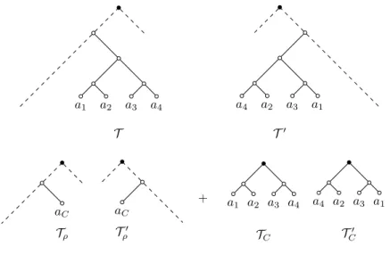
a1 a2 a3 a4 T a1 a3 a2 a4 T0 aC Tρ aC T0 ρ + a 1 a2 a3 a4 TC a1 a3 a2 a4 T0 C
Fig. 1 An example of the rooted cluster reduction. Black vertices are the respective roots.
phylogenetic X-trees T1 and T2 to be the minimum number of rSPR
opera-tions that are required to transform T1 into T2. We denote this distance by
drSPR(T1,T2). The associated decision problem is the following.
rSPR Distance
Input: Two rooted binary phylogenetic X-treesT and T0 and l∈ N.
Question: Is drSPR(T , T0)≤ l?
Our second theorem is an analogue of Theorem 1 for rSPR Distance instead of Hybridization Number. However, in order to define the required param-eter, the rSPR level of two rooted binary phylogenetic X-trees, we need to define a cluster reduction, following [5].
Definition 1 (rooted cluster reduction) LetT and T0 be rooted binary
phylogenetic X-trees and let C be a non-trivial cluster common to both T and T0. A cluster reduction is the operation of splitting (T , T0) into the two
pairs of smaller trees (TC,TC0), (Tρ,Tρ0) := (T |C, T0|C), (T ↓C,T0↓C). Note that
(TC,TC0) is a pair of phylogenetic C-trees, and (Tρ,Tρ0) is a pair of phylogenetic
((X\C)∪{aC})-trees that contain the original roots of T and T0 respectively.
See Fig. 1 for an example.
We now define a cluster sequence, which is essentially the result of applying several cluster reductions to a pair of trees. Let T and T0 be rooted binary
phylogenetic X-trees. Set ˆT0 =T and ˆT00 =T0. For a cluster sequence
con-sisting of t reductions, for i = 1, . . . , t let Ai be a non-trivial cluster common
to both ˆTi−1 and ˆTi0−1, and define Ti := ˆTi−1|Ai and Ti0 := ˆT0|Ai, and also
ˆ
Ti:= ˆTi−1↓Ai and ˆT
0
i := ˆTi0−1↓Ai, where the newly created leaf in ˆTiand ˆT
0 i is
labelled by ai. Finally, we denote ( ˆTt, ˆTt0) as (Tρ,Tρ0), to emphasize that these
two trees contain the original roots ofT and T0. The result is a sequence of
pairs of trees (T1,T10), . . . , (Tt,Tt0), (Tρ,Tρ0) which we call a cluster sequence.
Note that the leaf set of Ti and Ti0 is Ai and the leaf set of Tρ and Tρ0 is
(X∪S
i{ai}) \SiAi.
We say a cluster sequence is a full cluster reduction ofT and T0 if at each
step the cluster Ai is a minimal non-trivial common cluster and the trees Tρ
andT0
ρ contain no further non-trivial common clusters. Observe that the full
cluster reduction is unique, up to the ordering of pairs, since any non-trivial common cluster of T and T0 will at some point become minimal (once all
common subclusters have been reduced), and it will then itself be reduced. In addition, no pair (Ti,Ti0) in the full cluster reduction contains a non-trivial
common cluster.
For two rooted binary phylogenetic X-trees T and T0, the rSPR level is
the maximum rSPR distance between a pair of trees in a full cluster reduction ofT and T0, i.e. the maximum of d
rSPR(Ti,Ti0) over i∈ {1, . . . , t, ρ}. We may
now state the second theorem of the paper whose proof is deferred to Section 4. Theorem 2 Let T and T0 be two rooted binary phylogenetic X-trees. rSPR Distance is fixed-parameter tractable with respect to the rSPR level ofT and T0.
Note that, analogous to the hybridization number, the rSPR level of a pair of trees is at most the rSPR distance between the trees, and may be much smaller, even 1 for trees that have arbitrarily large rSPR distance. Plugging in current results for rSPR Distance [9], Theorem 2 implies the following. Corollary 2 LetT and T0 be two rooted binary phylogeneticX-trees. rSPR Distance can be solved in time O(2.344k· n), where n is the size of the leaf set ofT and k is the rSPR level of T and T0.
The TBR Problem. Let T be an unrooted binary phylogenetic X-tree and e = {u, v} be an edge of T such that neither u nor v is a leaf. Let T0 be
the unrooted binary phylogenetic X-tree obtained fromT by deleting e and reconnecting the subtreesTu andTv by
(i) subdividing an edge ofTu with a new vertex w,
(ii) subdividing an edge ofTv with a new vertex z,
(iii) adding the edge{w, z}, and
(iv) suppressing any vertices of degree two.
The decision problem TBR Distance is formally stated as follows. TBR Distance
Input: Two unrooted binary phylogenetic X-treesT and T0and l∈ N.
Note that the notions of displaying, hybridization number and hybridization level of two unrooted trees are defined as in the rooted framework. Our third theorem is an analogue of Theorem 1 for TBR Distance instead of Hy-bridization Number.
Theorem 3 LetT and T0be two unrooted binary phylogeneticX-trees. TBR Distance is fixed-parameter tractable with respect to the hybridization level of T and T0.
Plugging in current results for TBR Distance [8], Theorem 3 implies the following.
Corollary 3 LetT and T0be two unrooted binary phylogeneticX-trees. TBR Distance can be solved in time O(3k· n), where n is the size of the leaf set of T and k is the hybridization level of T and T0.
Note that the unrooted hybridization level is always smaller or equal to the TBR distance, since the unrooted hybridization number equals the TBR distance (see Theorem 6 in Section 5).
3 Proof of Theorem 1
The following lemma shows how the cluster reduction can be used as part of a divide-and-conquer approach to computing the hybridization number. Lemma 1 ([3]) Let T and T0 be two rooted binary phylogenetic X-trees. Suppose thatC⊂ X is a cluster of both T and T0, where (T
C,TC0)and (Tρ,Tρ0)
are the results of performing a cluster reduction of C on (T , T0). Then,
h(T , T0) = h(TC,TC0) + h(Tρ,Tρ0).
A straightforward consequence of Lemma 1 is that if (T1,T10),· · · , (Tt,Tt0),
(Tρ,Tρ0) is a cluster sequence ofT and T0, then
h(T , T0) = h(T
1,T10) +· · · + h(Tt,Tt0) + h(Tρ,Tρ0).
Next, we show that the hybridization level of two rooted binary phylo-genetic X-trees T and T0 is equal to the maximum hybridization number
between a pair of trees in a full cluster reduction of T and T0. Recall that,
for a rooted phylogenetic network N , its level is the maximum number of reticulation vertices in any biconnected component of N .
Lemma 2 Let T and T0 be two rooted binary phylogenetic X-trees and let (T1,T10), . . . , (Tt,Tt0), (Tρ,Tρ0) be a full cluster reduction of T and T0. Then,
the hybridization level of T and T0 equals max
i∈{1,...,t,ρ}h(Ti,T 0 i).
Proof For each i∈ {1, . . . , t}, let Ni be a rooted phylogenetic network
display-ing Ti and Ti0 with hybridization number h(Ti,Ti0) and let Ai and ai denote
the set of leaves of Ti and the new leaf created to represent the cluster Ai in
the ith cluster reduction, respectively. We may now rebuild a rooted
phylo-genetic network N displayingT and T0 from the smaller rooted phylogenetic
networks Ni as follows. We start with N = Nρ. While N contains a leaf v
labelled ai for some i, we replace v by a pendant copy of Niin N . Since each
arc incident with such a leaf is a cut arc of the resulting rooted phylogenetic network N , each biconnected component of N is a subnetwork of Ni for some
i∈ {1, . . . , t, ρ}. Thus, N displays T and T0 and the level of N is at most the
maximum of h(Ti,Ti0) over i∈ {1, . . . , t, ρ}, hence the hybridization level of T
andT0 is at most the maximum of h(T
i,Ti0) over i∈ {1, . . . , t, ρ}.
Conversely, let N be any rooted phylogenetic network displayingT and T0
and let k denote its level. Let the vertex set of N be V and the root be ρ. We will construct a cluster sequence forT and T0. Each cut arc (u, v) of N gives
rise to a cluster c(v) which is a common cluster toT and T0. A cut arc (u, v)
of N is trivial if v is a leaf of N , and it is a minimal non-trivial cut arc if there is no other non-trivial cut arc (w, x) of N such that there is a directed path from v to w in N . We obtain a cluster sequence forT and T0 by iteratively:
– selecting v in V at the head of a minimal non-trivial cut arc of N , which gives rise to c(v), a minimal non-trivial common cluster ofT and T0;
– performing the cluster reduction ofT and T0by c(v) replacing the cluster
with a new vertex cv, and
– replacing the subnetwork below the cut edge with a single pendant leaf cv
in N
Note that the deleted subnetwork is either a subtree (in fact, due to minimality, just a pair of leaves with a common parent, which is known as a cherry) or a biconnected component of N with pendant leaves, since otherwise, we could choose a smaller common cluster. Since the level of the network is k, this subnetwork of N is a phylogenetic network on c(v) containing at most k hybridization vertices and displayingT |c(v) and T0|c(v). Hence the cluster
pair in the cluster reduction has hybridization number at most k. We repeat this process until N has no further cut arcs, obtaining a cluster sequence (T1,T10), ..., (Tt,Tt0), (Tρ,Tρ0) forT and T0. Every cluster pair (Ti,Ti0) from the
cluster sequence has hybridization number at most k. It remains to consider the final pair (Tρ,Tρ0). Since in the end N had no (non-trivial) cut arcs, either
N was reduced to a cherry or N was a biconnected component with pendant leaves, and again we deduce that h(Tρ,Tρ0) ≤ k. Thus if T and T0 can be
displayed on a level-k phylogenetic network, then there is a cluster sequence forT and T0such that the maximum hybridization number between a pair of
trees in the cluster reduction is at most k.
It remains to show that the maximum hybridization number between a pair of trees in the full cluster reduction is therefore also at most k. We will make use of the fact that if a cluster reduction is not a reduction by a minimal non-trivial common cluster, then it can be broken down into a series of cluster
reductions each of which is by a minimal non-trivial common cluster. To see this consider a cluster reduction of T and T0 by a common cluster A and
suppose it is not a minimal non-trivial common cluster. Then, there is a subset A1⊂ A such that A1is a minimal non-trivial common cluster. We first reduce
by A1, obtaining (TA1,TA01), (Tρ,T
0
ρ), where there is a leaf a1 in Tρ and Tρ0
replacing the cluster A1. We may then reduce by the common cluster A∪
{a1} \ A1 of Tρ and Tρ0. This has broken the cluster reduction by A into a
minimal cluster reduction by A1 and a cluster reduction by a proper subset
of A. By repeating this process until the remaining reduction is itself by a minimal non-trivial common cluster, we iteratively break down the cluster reduction by A into a sequence of cluster reductions, each of which is by a minimal non-trivial common cluster.
So we first form a full cluster reduction from (T1,T10), ..., (Tt,Tt0), (Tρ,Tρ0)
by following the same sequence of cluster reductions used to create the cluster sequence, but at each step where we would reduceT and T0by a common
clus-ter A, we instead reduce by a sequence of minimal non-trivial common clusclus-ters, as described above, whose union contains all the elements of A. Finally, once we have finished breaking down the cluster reductions in the original cluster sequence, we continue to perform cluster reductions on Tρ and Tρ0 by any
re-maining minimal common clusters until none remain. The result is a full cluster reduction ( ˆT1, ˆT10), ..., ( ˆTs, ˆTs0), ( ˆTρ, ˆTρ0) such that each pair (Ti,Ti0) of the
orig-inal cluster sequence corresponds to a subsequence ( ˆTj, ˆTj0), . . . , ( ˆTq, ˆTq0) of the
full cluster reduction, in the sense that ( ˆTj, ˆTj0), . . . , ( ˆTq, ˆTq0) is itself a cluster
reduction of (Ti,Ti0). Then, by Lemma 1,
h(Ti,Ti0) = X j≤l≤q h( ˆTl, ˆTl0)≥ max j≤l≤qh( ˆTl, ˆT 0 l), implying k≥ max i∈{1,...,t,ρ}h(Ti,T 0 i)≥ max j∈{1,...,s,ρ}h( ˆTj, ˆT 0 j),
and, since this holds for every phylogenetic network N displaying T and T0,
whatever the level of N , the lemma follows. ut From Lemmas 1 and 2 it follows that there is a network displayingT and T0 minimizing the hybridization level that also minimizes the hybridization
number.
Lemma 3 Let T and T0 be two rooted binary phylogenetic X-trees. A full cluster reduction of T and T0 can be computed in time O(n), where n is the size of the leaf set of T .
Proof We start by applying the algorithm in [11] toT , which preprocesses T in time O(n) and creates a data structure that returns the least common ancestor (LCA) of any two specific vertices of T in O(1) time. Then, we compute, for each vertex x ofT , the number l(x) of leaves below it in O(n) total time. We do the same forT0. Finally, for each vertex x ofT , we store the vertex x0 of
T0 with x0 := LCA
T0(c(x)) as m(x). Since, assuming the children of x are y
and z, we have m(x) = LCAT0(m(y), m(z)), this can be done in O(n) time
via a post-order traversal ofT0 using the precomputed data structure. Then,
a cluster reduction ofT and T0 can be found as follows:
1 i← 1;
2 forx in a post-order traversal ofT do
3 if l(x)≥ 2, l(x) = l(m(x)) and x is not the root of T then
4 Ai← c(x);
5 (Ti,Ti0)← (TAi,TA0i);
6 reduce Ai to a single leaf ai in bothT and T0;
7 i← i + 1; 8 (Tρ,Tρ0)← (T , T0);
The overall worst-case running time of this algorithm is O(n); indeed, al-though there are O(n) iterations of the outer loop, each one involving reducing a cluster Ai of size O(n) in line 6, the sum of the sizes of the clusters is at
most O(n), and so the amortized running-time of this line is O(1). ut We are now in a position to prove Theorem 1 and Corollary 1.
Proof of Theorem 1 and Corollary 1Let the two rooted binary phyloge-netic X-trees T and T0 and the integer l be an instance of Hybridization
Number. Let|X| = n, and let k be the hybridization level of T and T0. We may first compute a full cluster reduction (T1,T10), ..., (Tt,Tt0), (Tρ,Tρ0) of T
andT0 in time O(n) by Lemma 3. We then apply the algorithm of [22] to each
pair (Ti,Ti0) to obtain h(Ti,Ti0) in time O(3.18h(Ti,T
0
i)· |Ti|). By Lemma 2,
h(Ti,Ti0)≤ k, and clearly
P
i|Ti| = O(n), hence we may compute h(T , T0) =
h(T1,T10) + ... + h(Tt,Tt0) + h(Tρ,Tρ0) in time O(3.18k· n). By a comparison of
h(T , T0) and l we may answer the decision problem in the same time bound,
and hence Hybridization Number is fixed parameter tractable when pa-rameterized by the hybridization level ofT and T0. ut
4 Proof of Theorem 2
Recall that, for solving instances of rSPR Distance with two rooted binary phylogenetic X-trees T and T0, we add to each of them a vertex labelled
by a dummy taxon lρ at the end of a pendant edge adjoined to the original
root. Given such an “augmented” treeT and a label x, let T |lρ→xdenote the
result of removing the vertex labelled lρ and replacing the label x by lρ. In
the following, we make use of the concept of rooted agreement forests: Given two rooted binary phylogenetic X-trees T and T0, a leaf-labelled forestF is
called a rooted agreement forest ofT and T0 ifF can be obtained from T and
T0, respectively, by a series of edge cuts as defined in Section 2. We say that a
rooted agreement forest is root-isolating if it contains the singleton tree that consists of the leaf labelled lρ. A rooted agreement forest for a cluster sequence
(T1,T10), ..., (Tt,Tt0), (Tρ,Tρ0) of two rooted binary phylogenetic X-treesT and
T0, is a leaf-labelled forestF on X ∪ {a
1, . . . , at} which can be obtained from
the forests{T1, ...,Tt,Tρ} and {T10, ...,Tt0,Tρ0} by a series of edge cuts.
For the proof of Theorem 2, we need to define the concept of cluster hierar-chy: the cluster hierarchy for a full cluster sequence (T1,T10), ..., (Tt,Tt0), (Tρ,Tρ0)
of two rooted binary phylogenetic X-treesT and T0 is defined as the directed
tree with a vertex for each component (Ti,Ti0) of the cluster sequence, and a
directed edge from vertex (Ti,Ti0) to vertex (Tj,Tj0) if a leaf labelled by aj is
present inT0
i. Then, by starting with (Tρ,Tρ0) as the root of the tree, and using
a breadth-first search, since t < n we have the following:
Observation 1 The cluster hierarchy for a full cluster sequence can be com-puted in timeO(n), where n is the size of the leaf set of T .
For the proof of Theorem 2, we will also make use of the Minimum-Weight Forest Algorithm of Linz and Semple [16], which establishes the correctness of the use of a cluster reduction in a divide-and-conquer approach for com-puting the rSPR distance. In particular, they offer the following theorem and algorithm.
Theorem 4 (Theorem 2.2 of [16]) Let T and T0 be two rooted binary phylogeneticX-trees. Let (T1,T10), ..., (Tt,Tt0), (Tρ,Tρ0) be a cluster sequence for
T and T0. Let G be a rooted agreement forest for this sequence of minimum
weightw(G). Then drSPR(T , T0) = w(G) − 1.
Algorithm Minimum-Weight Forest [16]
Input: A cluster sequence (T1,T10), ..., (Tt,Tt0), (Tρ,Tρ0) of two rooted binary
phylogenetic X-treesT and T0, along with its cluster hierarchy.
Output:The minimum weight of a rooted agreement forest for this sequence. Without needing to give a precise definition of a minimum-weight rooted agreement forest for a cluster sequence (for details see [16]), it suffices to note that if we start with two rooted binary phylogenetic X-treesT and T0, first
compute a full cluster reduction and its cluster hierarchy, and then apply the Minimum-Weight Forest algorithm, our output is one more than the rSPR distance between T and T0. It remains to bound the running time of this
approach. To do so, we need the following lemma:
Lemma 4 Let T and T0 be rooted binary phylogenetic X-trees and let x ∈ X. Then, there is a root-isolating rooted maximum-agreement forestF for T andT0 if and only ifdrSPR(T , T0) = drSPR(T |lρ→x,T0|lρ→x) + 1.
Proof LetT∗:=T |lρ→xandT∗0 :=T0|lρ→x.
“⇒”: Let F be a root-isolating rooted maximum-agreement forest for T and T0 and let T
ρ be the tree in F that consists of the singleton labelled lρ.
Then, drSPR(T , T0) = |F|. Let F0 be the result of removing Tρ from F and
relabelling the leaf labelled x by lρ. Clearly,F0 is a rooted agreement forest
maximizes agreement, assume towards a contradiction that there is a rooted agreement forestF∗forT
∗andT∗0with|F∗| < |F0|. Then, relabelling the leaf
labelled lρ by x inF∗ and adding Tρ to F∗ yields a rooted agreement forest
forT and T0 with|F∗| + 1 < |F| components, contradicting optimality of F.
“⇐”: Let drSPR(T , T0) = drSPR(T∗,T∗0) + 1. We construct a root-isolating
rooted maximum-agreement forest F for T and T0. To this end, letF ∗ be a
rooted maximum-agreement forest for T∗ and T∗0 and let F be the result of
relabelling the leaf labelled lρby x inF∗and adding a singleton tree whose only
vertex is labelled lρ. Then,|F| = |F∗| + 1 = drSPR(T∗,T∗0) + 1 = drSPR(T , T0).
Thus,F is a root-isolating rooted maximum-agreement forest for T and T0.
u t We have now all the building blocks to prove the main results of this section. Proof of Theorem 2 and Corollary 2.Let the two rooted binary phyloge-netic X-treesT and T0 and the integer l be an instance of rSPR Distance.
Let |X| = n, and let k be the rSPR level of T and T0. We may first
com-pute a full cluster reduction (T1,T10), ..., (Tt,Tt0), (Tρ,Tρ0) ofT and T0 and its
cluster hierarchy in time O(n) by Lemma 3 and Observation 1. We then ap-ply the algorithm of [16] to obtain drSPR(T , T0). The time-consuming step in
this algorithm is finding a maximum-agreement forest for each pairTi,Ti0 (if
possible a root-isolating one). These may be found, using Lemma 4, in time O(2.344drSPR(Ti,Ti0)·|Ti|) by the approach of [9]. By definition, drSPR(Ti,T0
i)≤ k
and, clearly,|Ti| ∈ O(n). Hence, the whole algorithm runs in time O(2.344k·n).
By a comparison of drSPR(T , T0) and l we may answer the decision problem in
the same time bound, and hence rSPR Distance is fixed parameter tractable when parameterized by the rSPR level ofT and T0. ut
Note that the hybridization number of two trees is always bigger than their rSPR distance [2], and so Lemma 2 and Corollary 2 imply the following: Corollary 4 LetT and T0 be two rooted binary phylogeneticX-trees. rSPR Distance can be solved in time O(2.344k· n), where n is the size of the leaf set ofT and k is the hybridization level of T and T0.
Note also that the authors of [22] claim to have an algorithm to solve rSPR Distance in O(2drSPR(T ,T0)· n) [23]. If this is true, the running time
in Corollaries 2 and 4 will reduce to O(2k
· n).
5 Proof of Theorem 3
In this section, we consider unrooted binary phylogenetic X-trees. Note that each edge e of any phylogenetic X-tree uniquely partitions X into nonempty sets C and C := X\ C such that all paths between a leaf labelled with an element of C and a leaf labelled with an element of C contain e. A set C for which such an edge exists in T is called a cluster of T . A cluster is called trivial if |C| = 1 or |C| = 1. Given an unrooted binary phylogenetic X-tree
T and a nontrivial cluster C of T , let T |C denote the minimal subtree of T containing each leaf whose label is in C (analogous to the rooted case) and denote by T ↓C the unrooted phylogenetic tree where T |C has been replaced
by a leaf labelled by aC. An unrooted agreement forest (uAF) for two unrooted
phylogenetic X-trees is the unrooted version of a rooted agreement forest: it is a leaf-labelled forestF that can be obtained from T and T0, respectively,
by a series of edge deletions, deletions of unlabeled leaves, and suppressions of degree-two vertices. A uAF of minimal cardinality is called an unrooted maximum-agreement forest (uMAF). F is said to isolate some x ∈ X if F contains a singleton tree consisting of the leaf labelled x (denoted by{x} ∈ F). Finally, we denote the number of trees inF by |F|.
In the following, we describe a cluster reduction for unrooted binary phy-logenetic trees, slightly different from the rooted case.
Definition 2 (unrooted cluster reduction) Let T and T0 be unrooted binary phylogenetic trees and let C be a non-trivial cluster common to both T and T0 (note that C is also a common cluster of T and T0). A cluster
reductionis the operation of splitting (T , T0) into the two pairs of smaller trees
(TC,TC0), (TC,TC0) := (T ↓C,T 0↓
C), (T ↓C,T0↓C). See Fig. 2 for an example.
Analogously to the rooted case, we call the result (T1,T10), . . . , (Tt,Tt0) of
repeatedly applying the cluster reduction to two unrooted binary phylogenetic treesT and T0 a cluster sequence forT and T0 and such a sequence is called
full if each cluster reduction leading to the sequence reduces a minimal non-trivial common cluster and the treesTtandTt0 contain no further non-trivial
common clusters. Again, the full cluster reduction is unique, up to the ordering of pairs and no pair (Ti,Ti0) in the full cluster reduction contains a non-trivial
common cluster.
Note that an unrooted cluster sequence can be computed as described in Lemma 3 by previously rooting the two trees on the same leaf.
The following results are fundamental for proving that TBR Distance is FPT in the hybridization level.
Theorem 5 ([1]) LetT and T0 be two unrooted binary phylogeneticX-trees. Let F be a uMAF for T and T0. ThendTBR(T , T0) =|F| − 1.
Theorem 6 ([13]) Let T and T0 be unrooted binary phylogenetic X-trees. Thenh(T , T0) = d
TBR(T , T0).
Note that the concepts of hybridization number and level refer to the undi-rected versions. The following observation is straightforward.
Observation 2 A forestF = {F1, . . . , Fk} is a uAF of T and T0if and only if
1. each tree ofF is displayed by both T and T0, 2. all labels ofT and T0 occur inF, and
3. the subtreesT (L(F1)), . . . ,T (L(Fk)) andT0(L(F1)), . . . ,T0(L(Fk)) are all
a1 a2 a3 a4 T T |C a1 a3 a2 a4 T0 T0|C aC T |C T ↓C aC T0|C T0↓C + aC a1 a2 a3 a4 T ↓C aC a1 a3 a2 a4 T0↓ C
Fig. 2 An example of an unrooted cluster reduction. The common cluster is C = {a1, a2, a3, a4}.
The following two lemmas constitute a portation of Lemma 4 and Lemma 1 to unrooted binary phylogenetic trees.
Lemma 5 Let T and T0 be unrooted binary phylogeneticX-trees and let x∈ X. If there is a uMAFF for T and T0 that isolates x, then
dTBR(T , T0) = dTBR(T |(X − x), T0|(X − x)) + 1
and, otherwise,
dTBR(T , T0) = dTBR(T |(X − x), T0|(X − x)).
Proof LetF0 be a uMAF forT |(X − x) and T0|(X − x).
First, suppose that there is a uMAFF for T and T0 that isolates x. Then,
F can be turned into a uAF for T |(X − x) and T0|(X − x) by deleting the
singleton tree containing x andF0can be turned into a uAF forT and T0 by
adding a singleton tree containing a vertex labelled x. Thus,|F| = |F0| + 1.
Next, suppose that there is no uMAF for T and T0 that isolates x and
vertex labelled x to F0 yields a uAF for T and T0 that isolates x, we have
|F| < |F0| + 1. However, since removing x from the tree of F that contains
x yields a uAF forT |(X − x) and T0|(X − x), we also have |F| ≥ |F0|. Thus,
|F| = |F0|. The lemma follows by Theorem 5. ut
Lemma 6 LetT and T0 be unrooted binary phylogeneticX-trees and let C be a nontrivial cluster of T and T0. If there is a uMAF forT ↓C andT0↓C that
isolates the leaf labelledaC, then
dTBR(T , T0) = dTBR(T ↓C,T0↓C) + dTBR(T |C, T0|C),
and, otherwise,
dTBR(T , T0) = dTBR(T ↓C,T0↓C) + dTBR(T ↓C,T0↓C).
Proof First off, suppose that there is a uMAF forT ↓C andT0↓C that isolates
the leaf labelled aC.
“≤”: Let FC be a uMAF for T |C and T0|C. Let FC be analogous for C.
LetF0 :=F
C] FC. Then, all trees of F0 are displayed byT and T0 and by
Observation 2,F0 is a uAF forT and T0. Thus,
dTBR(T , T0)≤ |F0| − 1 =|FC| + |FC| − 1 Theorem 5 = dTBR(T |C, T0|C) + dTBR(T |C, T0|C) + 1 Lemma 5 = dTBR(T ↓C,T0↓C) + dTBR(T |C, T0|C)
“≥”: Let F be a uMAF for T and T0. LetF(C) denote the set containing
exactly the trees ofF that contain only leaves labelled by elements of C. Let F(C) be defined analogously for C.
Case 1:F = F(C)]F(C). Then, | uMAF(T |C, T0|C)| = |F(C)| since, oth-erwise, exchangingF(C) for a uMAF of T |C and T0|C in F yields a uAF that is
smaller thanF, contradicting optimality of F. Likewise, | uMAF(T |C, T0|C)| =
|F(C)|. Then, dTBR(T , T0) =|F| − 1 = |F(C)| + |F(C)| − 1 Theorem 5 = dTBR(T |C, T0|C) + dTBR(T |C, T0|C) + 1 Lemma 5 = dTBR(T ↓C,T0↓C) + dTBR(T |C, T0|C)
Case 2:There is a tree H inF containing a leaf labelled x ∈ C and a leaf labelled y∈ C (note that only one of such “mixed” trees can be present in F; indeed, since C is a cluster of both trees, the existence of two such trees will contradict Condition 3 of Observation 2). Then, F = F(C) ] F(C) ] {H}. Let H↓C denote the result of contracting all edges of H that are on a path
between two leaves with labels of C in H and labelling the vertex on which they are all contracted with C. Let H↓C be analogous for C. Then, all labels of C and the special label aC occur in F1 :=F(C) ] {H↓C} and all its trees
are displayed byT ↓CandT0↓
C. Thus, by Observation 2,F1is a uAF forT ↓C
andT0↓
C. Likewise, F(C) ] {H↓C} is a uAF for T ↓C andT0↓C. Thus,
dTBR(T , T0) =|F| − 1 = |F(C) ] F(C) ] {H}| − 1
=|F(C) ] {H↓C}| + |F(C) ] {H↓C}| − 2
≥ dTBR(T ↓C,T0↓C) + dTBR(T ↓C,T0↓C)
≥ dTBR(T ↓C,T0↓C) + dTBR(T |C, T0|C)
Next, suppose that there is no uMAF forT ↓C andT0↓C that isolates the
leaf labelled aC.
“≤”: First, note that if there is a uMAF for T ↓C and T0↓C that isolates
the leaf labelled aC, the first part of our proof implies that dTBR(T , T0) = dTBR(T |C, T0|C) + dTBR(T ↓C,T0↓C)
≤ dTBR(T ↓C,T0↓C) + dTBR(T ↓C,T0↓C).
Now, let consider the case where there is no uMAF for T ↓C and T0↓C
(respectively T ↓C and T0↓C) that isolates the leaf labelled aC (respectively
labelled aC). LetFC be a uMAF for T ↓C and T0↓C and let HC denote the
tree of FC containing the label aC. Let FC and HC be analogous for C.
Let H be the result of joining HC and HC by identifying the leaves labelled
aC and aC, respectively and suppressing this degree-two vertex. Let F0 :=
(FC\ {HC}) ] (FC\ {HC}) ] {H}. Then, H is displayed by T and T0 and,
thus, all trees ofF0 are displayed byT and T0. Moreover, it is easy to see that
T (H) is vertex disjoint with the other trees in the forest, and the same holds forT0(H). Then, by Observation 2,F0 is a uAF forT and T0. Thus,
dTBR(T , T0)≤ |F0| − 1 =|FC\ {HC}| + |FC\ {HC}| + |{H}| − 1 =|FC| + |FC| − 2 = dTBR(T |C, T0|C) + dTBR(T |C, T0|C) Lemma 5 = dTBR(T ↓C,T0↓C) + dTBR(T ↓C,T0↓C)
“≥”: Let F be a uMAF for T and T0. LetF(C) denote the set containing
exactly the trees ofF that contain only leaves labelled by elements of C. Let F(C) be defined analogously for C.
Case 1:F = F(C)]F(C). Then, | uMAF(T |C, T0|C)| = |F(C)| since, oth-erwise, exchangingF(C) for a uMAF of T |C and T0|C in F yields a uAF that is
smaller thanF, contradicting optimality of F. Likewise, | uMAF(T |C, T0|C)| =
|F(C)|. Let F0(C) be a uMAF forT ↓
C andT0↓Cand note that, by Lemma 5
|F0(C)| = |F(C)|. Further, let F0(C) be a uMAF forT ↓
C andT0↓C and note
that|F0(C)| ≤ |F(C)| + 1. Then,
dTBR(T , T0) =|F| − 1 = |F(C)| + |F(C)| − 1
≥ |F0(C)| + |F0(C)| − 2
Case 2:There is a tree H inF containing a leaf labelled x ∈ C and a leaf labelled y∈ C. This is completely analogous to Case 2 above. ut It is worth mentioning that, in the two cases of Lemma 6, the TBR dis-tances differ by exactly one, that is, dTBR(T |C, T0|C) ≤ dTBR(T ↓C,T0↓C)≤
dTBR(T |C, T0|C) + 1, Lemma 6 implies that, if there is a uMAF for T ↓C and
T0↓
C that isolates the leaf labelled aC and a uMAF for T ↓C and T0↓C that
isolates the leaf labelled aC, then, when gluing the forests of the subtrees back together to form a uMAFF for T and T0, then we have a tree that does not
contain any labelled leaf. Thus, an optimal uMAF has size|F|−1. This means that, to minimize the size of a forest forT and T0, we need to favor the forests
isolating the dummy taxa. Then, we have the following:
Corollary 5 LetT and T0be unrooted binary phylogeneticX-trees. Let (T1,T10),
. . . , (Tt,Tt0) be a cluster sequence ofT and T0. LetF be a maximum-agreement
forest of T and T0. Fori∈ {1, . . . , t}, let Fi be a maximum-agreement forest
for Ti and Ti0 such that r :=|{C : {aC}, {aC} ∈ UiFi}| is maximal. Then,
dTBR(T , T0) = (Pi|Fi|) − t − r.
Corollary 5 is a drop-in replacement for Theorem 2.2 in [16] and lets us use the entire cluster-sequence-based machinery of [16] for unrooted phylogenetic trees. Thus, a slight modification of the Minimum-Weight Forest algorithm of [16] (solving the TBR Distance instead of the rSPR Distance and using the unrooted cluster reduction instead of the rooted one) leads right to the following theorem:
Theorem 7 Let T and T0 be two unrooted binary phylogenetic X-trees and let (T1,T10), . . . , (Tt,Tt0) be a full cluster reduction of T and T0. Then, the
hybridization level of T and T0 equals max
i∈{1,...,t}dTBR(Ti,T 0 i).
Proof First, from Lemma 6, we have that max i∈{1,...,t}dTBR(Ti,T 0 i) = max i∈{1,...,t}h(Ti,T 0 i).
The fact that maxi∈{1,...,t}h(Ti,Ti0) equals the hybridization level ofT and T0
can be proven similarly to Lemma 2, and we do not repeat the proof here. ut Thanks to Theorem 7, Theorem 3 and Corollary 3 can be proven simi-larly to Theorem 2 and Corollary 2, since TBR Distance can be solved in O(3k
· n), where k is the TBR distance of T and T0 [8].
6 Conclusion
In this paper, we have shown better bounds for the running time of algorithms computing the hybridization number and the rSPR/TBR distance between two
phylogenetic trees using cluster reductions. We have thus given an explanation for the curious divergence between theoretical results and observed running time of algorithms using cluster reductions.
A deeper biological question that warrants further research is: why does real biological data partition so effectively under the cluster reduction? In other words, why are observed networks of low hybridization level?
Acknowledgment
The third author gratefully acknowledges the scholarship supplied to her from the Republic of Turkey, Ministry of National Education.
Part of the work has been conceived at the 7th workshop on Graph Classes, Optimization, and Width Parameters.
References
1. Allen BL, Steel M (2001) Subtree transfer operations and their induced metrics on evolutionary trees. Annals of combinatorics 5(1):1–15
2. Baroni M, Gr¨unewald S, Moulton V, Semple C (2005) Bounding the num-ber of hybridisation events for a consistent evolutionary history. Journal of mathematical biology 51(2):171–182
3. Baroni M, Semple C, Steel M (2006) Hybrids in real time. Systematic Biology 55(1):46–56
4. Bordewich M, Semple C (2005) On the computational complexity of the rooted subtree prune and regraft distance. Annals of combinatorics 8(4):409–423
5. Bordewich M, Semple C (2007) Computing the hybridization number of two phylogenetic trees is fixed-parameter tractable. IEEE/ACM Transac-tions on Computational Biology and Bioinformatics (TCBB) 4(3):458–466 6. Bordewich M, Semple C (2007) Computing the minimum number of hy-bridization events for a consistent evolutionary history. Discrete Applied Mathematics 155(8):914–928
7. Bordewich M, Linz S, John KS, Semple C (2007) A reduction algorithm for computing the hybridization number of two trees. Evolutionary bioin-formatics online 3:86
8. Chen J, Fan JH, Sze SH (2013) Parameterized and approximation algo-rithms for the MAF problem in multifurcating trees. In: Graph-Theoretic Concepts in Computer Science, Springer, pp 152–164
9. Chen ZZ, Fan Y, Wang L (2013) Faster exact computation of rSPR dis-tance. Journal of Combinatorial Optimization 29(3):605–635
10. Hallett MT, Lagergren J (2001) Efficient algorithms for lateral gene trans-fer problems. In: Proceedings of the fifth annual international contrans-ference on Computational biology, ACM, pp 149–156
11. Harel D, Tarjan RE (1984) Fast algorithms for finding nearest common ancestors. siam Journal on Computing 13(2):338–355
12. Hein J, Jiang T, Wang L, Zhang K (1996) On the complexity of comparing evolutionary trees. Discrete Applied Mathematics 71(1):153–169
13. van Iersel L, Kelk S, Stougie L, Boes O (In preparation) On unrooted and root-uncertain variants of several well-known phylogenetic network problems
14. Jansson J, Sung WK (2006) Inferring a level-1 phylogenetic network from a dense set of rooted triplets. Theoretical Computer Science 363(1):60–68 15. Kelk S, Scornavacca C, Van Iersel L (2012) On the elusiveness of clusters. IEEE/ACM Transactions on Computational Biology and Bioinformatics (TCBB) 9(2):517–534
16. Linz S, Semple C (2011) A cluster reduction for computing the subtree distance between phylogenies. Annals of Combinatorics 15(3):465–484 17. Maddison WP (1997) Gene trees in species trees. Systematic biology
46(3):523–536
18. Nakhleh L, Warnow T, Linder CR (2004) Reconstructing reticulate evolu-tion in species: theory and practice. In: Proceedings of the eighth annual international conference on Resaerch in computational molecular biology, ACM, pp 337–346
19. Semple C, Steel MA (2003) Phylogenetics, vol 24. Oxford University Press 20. Van Iersel L, Kelk S (2011) When two trees go to war. Journal of
Theo-retical Biology 269(1):245–255
21. Van Iersel L, Kelk S, Mnich M (2009) Uniqueness, intractability and exact algorithms: reflections on level-k phylogenetic networks. Journal of Bioin-formatics and Computational Biology 7(04):597–623
22. Whidden C, Beiko RG, Zeh N (2013) Fixed-parameter algorithms for max-imum agreement forests. SIAM Journal on Computing 42(4):1431–1466 23. Whidden C, Beiko R, Zeh N (In preparation) Computing the SPR distance