HAL Id: inria-00417713
https://hal.inria.fr/inria-00417713
Submitted on 16 Sep 2009
HAL is a multi-disciplinary open access
archive for the deposit and dissemination of
sci-entific research documents, whether they are
pub-lished or not. The documents may come from
teaching and research institutions in France or
abroad, or from public or private research centers.
L’archive ouverte pluridisciplinaire HAL, est
destinée au dépôt et à la diffusion de documents
scientifiques de niveau recherche, publiés ou non,
émanant des établissements d’enseignement et de
recherche français ou étrangers, des laboratoires
publics ou privés.
Smoothing techniques for convex problems.
Applications in image processing.
Pierre Weiss, Mikael Carlavan, Laure Blanc-Féraud, Josiane Zerubia
To cite this version:
Pierre Weiss, Mikael Carlavan, Laure Blanc-Féraud, Josiane Zerubia. Smoothing techniques for convex
problems. Applications in image processing.. SAMPTA, May 2009, Marseille, France. �inria-00417713�
Smoothing techniques for convex problems.
Applications in image processing.
Pierre Weiss
(1), Mika¨el Carlavan
(2), Laure Blanc-F´eraud
(2)and Josiane Zerubia
(2)(1) Institute for Computational Mathematics, Kowloon Tong, Hong Kong.
(2) Projet Ariana - CNRS/INRIA/UNSA, 2004 route des Lucioles, 06902 Sophia-Antipolis, France. (1) [email protected], (2) [email protected]
Abstract:
In this paper, we present two algorithms to solve some inverse problems coming from the field of image process-ing. The problems we study are convex and can be ex-pressed simply as sums of lp-norms (p ∈ {1, 2, ∞}) of
affine transforms of the image. We propose 2 different techniques. They are - to the best of our knowledge - new in the domain of image processing and one of them is new in the domain of mathematical programming. Both meth-ods converge to the set of minimizers. Additionally, we show that they converge at least as O¡1
N
¢
(where N is the iteration counter) which is in some sense an “optimal” rate of convergence. Finally, we compare these approaches to some others on a toy problem of image super-resolution with impulse noise.
1. Introduction
Many image processing tasks like reconstruction or seg-mentation can be done efficiently by solving convex opti-mization problems. Recently these models received con-siderable attention and this led to some breakthrough. Among them are the new sampling theorems [5] and the impressive results obtained using sparsity or regularity as-sumptions in image reconstruction (see e.g. [4]).
These results motivate an important research to accelerate the convergence speed of the minimization schemes. In the last decade, many algorithms like iterative threshold-ing or dual approaches were reinvented by the “imagthreshold-ing community” (see for instance [2, 3] for old references). Recently, the “mathematical programming community” got interested in those problems and it led to some drastic improvements. As examples let us cite the papers by Y. Nesterov [9, 10] and M. Teboulle [1] which improve by one order of magnitude most first order approaches. In this paper, we mainly follow the lines of Y. Nesterov [9]. We consider the problem of minimizing the sum of
lp-norms (p ∈ {1, 2, ∞}) of affine transforms of the
im-age. The general mechanism of the algorithms we propose consists in smoothing the problem and solve it with an ef-ficient first order scheme. Our contribution is mainly to extend the results of [9] to a more general setting and to propose a dual variant which behaves better in all prob-lems we tested. We also give convergence rates for the proposed algorithms. We believe, this gives some insight on the important factors that influence the algorithms effi-ciency and helps designing solvable problems.
2. The problems considered
In this paper, we consider the following seminal model of image deterioration:
u0= Du + b (1)
where u is an original, neat image, D : Rn → Rmis some
known linear transform, b ∈ Rm is some additive noise
and u0 ∈ Rm is a given observed image. This simple
formalism actually models many real situations. For in-stance, D can be an irregular sampling and a convolution. In this case recovering u from u0 is a super-resolution
problem [7]. Other applications include image inpainting, compression noise reduction, texture+cartoon decomposi-tions, reconstruction from noisy indirect measurements... Finding u from the observation u0is an inverse problem.
There exists many ways to solve it. In this paper, we con-centrate on two variational models. The first one consists in solving the following convex problem:
min x∈X ||Bx||1+ λ||Dx − u0||p | {z } Ψ(x) . (2)
The second one consists in solving: min y∈Y ¡ ||y||1+ λ||DB∗y − u0||p ¢ . (3) In both problems, B : Rn → Rois a linear transform, || ·
||pdenotes the standard lp-norm and X and Y are simple
convex sets (like Rnor [0, 1]n).
The interpretation of the first model is as follows: we look for an image x which minimizes ||Bx||1such that Dx is
close to u0. The function x 7→ ||Bx||
1can be seen as a
regularity a priori on the image. For instance, if B is the
discrete gradient, then it corresponds to the total variation. If B is some wavelet transform, it is equivalent to a Besov semi-norm [6]. p must be chosen depending on the statis-tics of the additive noise. For instance, p should be equal to 2 for Gaussian noise, to 1 for impulse noise and to ∞ for uniform noise.
The interpretation of the second model is the following: we look for a decomposition y of the restored image in some dictionary B∗ such that its reconstruction B∗y is
close to u0. Minimizing the l1-norm of y is known to
favor sparse structures. The underlying assumption is thus that the original image u is sparse in the dictionary B∗.
From a numerical point of view, both problems are very similar. However, the first one is slightly more general and complicated than the second. We will thus give a detailled analysis of its resolution and only provide numerical re-sults for the second one.
The remaining of the paper is as follows. We first present an algorithm based on a regularization of the primal prob-lem (2). Then we present a technique to regularize a dual version of (2). Finally we propose theoretical and numeri-cal comparisons of both techniques on a problem of image super-resolution. Due to space limitations, we only pro-vide the main ideas in this paper. We refer the reader to [12] (in French), for the proofs of the propositions.
3. Smoothing of the primal problem
In this section, we propose a method to minimize (2). Its principle is exactly the same as the method proposed by Y. Nesterov in [9]:
1. Smooth the non-differentiable terms in (2).
2. Solve the regularized problem using an accelerated gradient method.
The only difference is that we do not require the set X to be bounded, which requires a slightly different analysis. Now let us present some details of this approach. A key observation to solve (2) is that it can be rewritten as a so called min-max problem. Let p0 denote the conjugate of
p
³ i.e. 1
p0 +1p = 1
´
. We can rewrite problem (2) as fol-lows: min x∈X µ max y∈Y ¡ hBx, y1i + λhDx − u0, y2i ¢¶ (4) = min x∈X
maxy∈Y (hAx − h, yi)
| {z } Ψ(x) (5)
where h·, ·i denotes the canonical scalar product,
A = · B λD ¸ , h = · 0 λu0 ¸ and (6) Y = {y = (y1, y2) ∈ Ro×Rm, ||y1||∞≤ 1, ||y2||p0 ≤ 1}. (7) The function Ψ is a conjugate function and the set Y is bounded. It can thus be smoothed using a Moreau regular-ization. Let us denote:
Ψµ(x) = max y∈Y ³ hAx − h, yi −µ 2||y|| 2 2 ´ . (8) This function can be shown to be L-Lipschitz differen-tiable:
||∇Ψµ(x1) − ∇Ψµ(x2)||2≤ L||x1− x2||2 (9)
with L = |||A|||µ 2 and |||A||| = max
x∈Rn,||x||
2≤1
(||Ax||2).
Furthermore, it is a good uniform approximation of Ψ in the following sense:
0 ≤ Ψ(x) − Ψµ(x) ≤ µ 2D. (10) where D = µ max y∈Y ¡ ||y||2 2 ¢
. Thus, we can make the dif-ference between Ψ and Ψµas small as desired by
decreas-ing µ. The approximation Ψµ is actually very common
in image processing. For instance, when p = 1, it cor-responds to the approximation of the absolute value by a Huber function. When p = ∞ it is slightly more difficult, but it can still be computed in closed form.
The smoothed problem writes: min
x∈X(Ψµ(x)) . (11)
It consists in minimizing a differentiable function over a simple set. We can thus apply projected gradient like al-gorithms to solve it. Unfortunately, µ has to be chosen small in order to get a good approximate solution. This requires to use small step sizes in the gradient descent and thus results in a very slow convergence rate. The main observation of Y. Nesterov in [9] is that using an accel-erated version of the projected gradient methods can ac-tually compensate the approximation error. This results in a convergence rate in O¡1
N
¢
(where N is the iteration counter), while other first order approaches like projected subgradient descents converge as O
³ 1 √ N ´ .
Now let us write down the complete algorithm to solve (11). Let x∗
µdenote a solution of (11) (it is not unique in
general). We propose the following algorithm: Algorithm 1 (Primal)
Choose a number of iterations N .
Set a starting point x0(as close as possible to x∗ µ). Set µ = µ(N ) = |||A|||·||x0−x∗µ||2 N . Set A = 0, g = 0 and x = x0. for k = 0 to N do a = 1 L+ q 1 L2 +L2A v = ΠX ¡ x0− g¢ y = Ax+av A+a x = ΠX ³ y −∇Ψµ(y) L ´ g = g + a∇Ψµ(x) A = A + a end for Set xN = x.
Our main convergence results are as follows. Let x∗
de-note a solution of (2).
Proposition 1 xN converges to the set of minimizers of
(2).
Proposition 2 The worst case convergence rate is: Ψ(xN) − Ψ(x∗) ≤2|||A||| · ||x 0− x∗ µ||2 √ D N . (12)
Note that the distance ||x0 − x∗
µ||2 is unknown in
gen-eral, so that Algorithm 1 might not seem implementable. In the case where X is a compact set, this quantity can be bounded above by the diameter of X. When X is not bounded, it actually suffices to choose µ of order |||A|||N to
get a precision of order O¡N1¢. Algorithm (1) is thus im-plementable and converges as O¡1
N
¢
. This convergence rate is neatly sublinear and might seem bad at first sight. Actually, it is somehow optimal. Indeed, A. Nemirovski shows in [8] that some instances of problems like (5) can-not be solved with a better rate of convergence than O¡1
N
¢ using first order methods.
4. Smoothing of the dual problem
In this section, we propose an approach alternative to the previous one. Its flavor is similar to a proximal-method. One way to understand this scheme is that we smooth the “dual” problem instead of the primal problem. Note that the min and the max in equation (5) cannot be inverted as we do not suppose X to be compact. So we cannot use -properly speaking - the term dual problem.
Instead of solving (2), we solve: min x∈X ³ ||Bx||1+ λ||Dx − u0||p+ ² 2||x − x 0||2 2 ´ (13) where ² ∈ R+
∗ and x0 should be chosen close to the set
of minimizers of (2). It can be shown that as ² goes to 0, the unique solution of (13) converges to the Euclidean projection of x0onto the set of minimizers of (2). We can
rewrite (13) as a min-max problem: min
x∈X
µ max
y∈Y (hAx − h, yi) +
² 2||x − x 0||2 2 ¶ (14) = max y∈Y minx∈X ³ hAx − h, yi +² 2||x − x 0||2 2 ´ | {z } Ψ²(y) (15).
Note that we can invert the min and the max only because the term ²
2||x − x0||22 makes the problem coercive in x.
Now, the important observation is that the function Ψ² is
the conjugate of a strongly convex function. It is thus con-cave and Lipschitz differentiable:
||∇Ψ²(y1) − ∇Ψ²(y2)||2≤ L||x1− x2||2 (16)
∀(y1, y2) ∈ Y × Y with L ≤ |||A|||
2
² . Problem (15)
consists in maximizing a Lipschitz differentiable concave function over a convex set. It thus seems interesting to use a scheme similar to Algorithm 1 on this problem. Unfortu-nately we will get a convergence rate on the dual variable
y and not on the variable of interest: x(y) = arg min
x∈X ³ hAx − h, yi +² 2||x − x 0||2 2 ´ . (17)
Actually, a slight modification of Nesterov’s scheme (an ergodic version) can be shown to ensure convergence of
xN with the desired convergence rate. In the following,
we detail briefly our main results. Let x∗
²denote the solution of (13) and y∗²denote a solution
of (15). Let X∗denote the set of minimizers of (2) and let
us consider the following algorithm:
Algorithm 2 (Dual)
Choose a number of iterations N .
Set a point x0(as close as possible to X∗).
Set a starting point y0(as close as possible to y∗ ²). Set ² = ²(N ) = |||A|||·||x0−x∗²||2 N . Set A = 0, g = 0, ¯x = 0 and y = y0. for k = 0 to N do a = 1 L+ q 1 L2 +L2A v = ΠY ¡ y0− g¢ z = Ay+avA+a y = ΠY ³ z +∇Ψ²(z) L ´ ¯ x = ¯x + ax(y) (cf. equation (17)) g = g − a∇Ψ²(y) A = A + a end for Set ¯xN = x¯ A.
This algorithm can be shown to have the following prop-erties.
Proposition 3 ¯xN converges to the projection of x0onto
the set of minimizers of (2).
Proposition 4 The worst case convergence rate is: Ψ(¯xN) − Ψ(x∗) ≤ 2|||A||| · ||x 0− x∗ ²||2 √ D N . (18)
Rate (18) is actually very similar to (12). It is thus natural to wonder if there is an interest in using this dual approach. Let us present some interesting aspects of this scheme:
• In the dual approach, the solution of the regularized
problem is unique. This guarantees a certain stability of the iterates.
• We can show an additional convergence rate in norm
to the regularized solution. Namely, for a fixed ², we have for all k:
||¯xk− x∗ ²||22≤
D|||A|||
² · k2 (19)
• In practical experiments, model (13) with a small ²
leads to slightly better SNR than model (2) for some restoration purposes in image processing.
• The practical convergence rates of the dual approach
were better than those of the primal approach in all our experiments.
To conclude the theoretical part of this paper, let us pre-cise that problem (3) can be solved with the same algo-rithms. However, it is preferable not to regularize the term
y 7→ ||y||1which can be minimized using accelerated
soft-thresholding algorithms [1, 10, 12].
5. Numerical results
In this section we present some comparisons for a prob-lem of image zooming with impulse noise. To solve this problem, we simply set:
0 500 1000 1500 2000 2500 3000 3500 4000 4500 5000 10−3 10−2 10−1 100 101 102 103 104 Number of iterations Ψ (x k) − Ψ (x *) Nesterov Primal Nesterov Dual Projected Gradient Primal Projected Gradient Dual
Figure 1: Cost function w.r.t. the number of iterations.
• D: convolution by a low-pass filter followed by a
down sampling of factor d in the x and y directions.
• p = 1 (which is adapted to impulse noise).
• B: a redundant wavelet transform. We set B to be
the Dual-Tree Complex Wavelet Tranform (DTCW) [11].
In that case |||A|||2 can be computed explicitly. For the
general case, let us point out that iterated power algorithms provide good approximations of |||A∗A||| = |||A|||2.
In Figure 1, we chose ² = 0.045 and µ = 10−5. This
ensures that both methods lead to the same asymptotic ac-curacy (measured in terms of objective function). We can see that the dual approach seems to have a better behav-ior. For this problem reducing Ψ(x0) − Ψ(x∗) by a factor
103is enough for visual purposes. The dual Nesterov
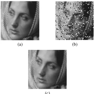
ap-proach requires 450 low cost iterations. The smoothing method proposed by Y. Nesterov requires 1700 iterations. The classical Cauchy steps requires much more than 5000 iterations to reach this goal. We can thus see the major improvement of Y. Nesterov’s scheme on these problems. We carried out many other experiments which led to the same conclusion. Figure 2 shows the solution of the prob-lem. The DTCW transform allows to retrieve thin details but slightly blurs the image. Further investigations will be led to address this issue.
6. Acknowledgments
The authors would like to thank the CS Compagny in Toulouse (France) for partial funding of this research work.
References:
[1] A. Beck and M. Teboulle. Fast iterative shrink-agethresholding algorithm for linear inverse prob-lems. SIAM J. on Imaging Science, to appear. [2] A. Bermudez and C. Moreno. Duality methods for
solving variational inequalities. Comp. and Maths.
with Appls., 7:43-58, 1981.
(a) (b)
(c)
Figure 2: Restoration of a down-sampled and noised im-age. (a) Original image, (b) down-sampled (by a factor 2) and noised image by 10% of ”Salt & Pepper” noise and finally (c) result of the Nesterov dual approach.
[3] R.J. Bruck. On the weak convergence of an ergodic iteration for the solution of variational inequalities for monotone operators in hilbert space. J. Math.
Anal. Appl, 61:159-164, 1977.
[4] J.F. Cai, R. Chan, Z.W. Shen, and L.X. Shen. Con-vergence analysis of tight framelet approach for missing data recoverys. Advances in Computational
Mathematics, to appear.
[5] E. Candes, J. Romberg, and T. Tao. Robust uncer-tainty principles: Exact signal reconstruction from highly incomplete frequency information. IEEE Inf.
Theory, 2006.
[6] A. Chambolle, R. Devore, N.Y. Lee, and B.J. Lucier. Nonlinear wavelet image processing: Variational problems, compression, and noise removal through wavelet shrinkage. IEEE Trans. Image Processing, 7:319-335, 1998.
[7] G. Facciolo, A. Almansa, J.-F. Aujol, and Vicent Caselles. Irregular to regular sampling, denoising and deconvolution. SIAM Journal on Multiscale Modeling and Simulation, in press.
[8] A. Nemirovski. Information-based complexity of linear operator equations. Journal of Complexity, 8:153-175, 1992.
[9] Y. Nesterov. Smooth minimization of non-smooth functions. Math. Program., 103(1):127-152, 2005. [10] Y. Nesterov. Gradient methods for minimizing
com-posite objective function. CORE Discussion Paper
2007/76, 2007.
[11] I. W. Selesnick, R. G. Baraniuk, and N. G. Kings-bury. The dual-tree complex wavelet transform.
IEEE Signal Processing Magazine, 22(6), Nov.
2005.
[12] P. Weiss. Algorithmes rapides d’optimisation
con-vexe. Applications `a la restauration d’images et `a la d´etection de changements. PhD thesis, Universit´e de