Decentralized control of multiple collaborating agents

Decentralized Control of Multiple Collaborating Agents

by

Henry Wong

Submitted to the Department of Electrical Engineering and Computer Science

in partial fulfillment of the requirements for the degree of

Bachelor of Science in Computer Science and Engineering

and Master of Science in Computer Science and Engineering

at the

MASSACHUSETTS INSTITUTE OF TECHNOLOGY

June 2001

@ Henry Wong, MMI. All rights reserved.

The author hereby grants to MIT permission to reproduce and distribute publicly paper

and electronic copies of this thesis document in whole or in part.

A u th or ... . ...

Department of Electrical Engineering and Coji ter Scienc

May 18, 2001

Certified by.

Certified by. .

...

...

... ... ....

Dr. Michael Cleary

Sei' r Member of Technical Staff, Draper Laboratory

Thesis Supervisor

...

. ... ..

.".W

.. ...

Leslie Pack Kaelbling

Professor, MIT Artifical Intelligence Laboratory

Thesis Supervisor

I

Accepted by ... ...-.

Arthur C. Smith

Chairman, Department Committee on Graduate Theses

MASSACHUSETTS INSTITUTE OF TECHNOLOGY

MIT

L-ib

ries

Document Services

DISCLAIMER OF QUALITY

Due to the condition of the original material, there are unavoidable

flaws in this reproduction. We have made every effort possible to

provide you with the best copy available. If you are dissatisfied with

this product and find it unusable, please contact Document Services as

soon as possible.

Thank you.

The images contained in this document are of

the best quality available.

* Archives copy of this thesis contains grayscale images only.

Decentralized Control of Multiple Collaborating Agents

by

Henry Wong

Submitted to the Department of Electrical Engineering and Computer Science on May 18, 2001, in partial fulfillment of the

requirements for the degree of

Bachelor of Science in Computer Science and Engineering and Master of Science in Computer Science and Engineering

Abstract

This thesis investigates the effect of various factors on multi-agent collaboration in a simulated fire-fighting domain. A simulator was written that models fires and fire-fighting agents in an area of a few square city blocks. Different scenarios were constructed to test the effects of limiting the agents' knowledge and to compare the effects of coordinating the agents through a single entity with the results obtained through independent decision making. This research demonstrates that the amount of information available to each agent and the agents' ability to act on this information are typically much more important factors than the use of a complex planning mechanism; as long as the agents are aware of each other and take minimal steps to coordinate their actions they are able to achieve results that are nearly as good as those achieved by much more complicated algorithms.

Thesis Supervisor: Dr. Michael Cleary

Title: Senior Member of Technical Staff, Draper Laboratory

Thesis Supervisor: Leslie Pack Kaelbling

Acknowledgments

I'd like thank my supervisor, Michael Cleary, for his invaluable guidance and technical advice. I'd also like to thank Micheal Cleary and Mark Abramson for making a Draper Fellowship available

to me, for giving me a topic to explore and for all of their support and enthusiasm towards my thesis.

I'd also like to thank my MIT advisor, Dr. Leslie Kaelbling, for explaining some of the harder parts of the mathematics to me and for providing constant advice on how I could improve my thesis and what steps I should take in order to accomplish the most in the given amount of time.

This thesis was supported by The Charles Stark Draper Laboratory Inc., under IR&D 13024. Publication of this thesis does not constitute approval by The Charles Stark Draper Laboratory, Inc., of the findings or conclusions contained herein. It is published for the exchange and stimulation of ideas.

Permission is hereby granted by the Author to the Massaschusetts Institute of Technology to reproduce any or all of this thesis.

Contents

1 Introduction

2 Related Work in Fire Suppression

2.1 Previous Fire Models . . . . 2.1.1 A Simple Grid of Cells . . . .

2.1.2 Rothermel's Work . . . .

2.1.3 The RoboCup Rescue Simulator . . . .

3 The Simulator and Fire Model

3.1 The Simulator Engine . . . . 3.2 The Hybrid Fire Model . . . . 4 The cost of moving agents during a single action

4.1 Overview of the stepping stone algorithm... 4.1.1 Step 1 -Initial Solution . . . .

4.1.2 Step 2 -Basic Cells . . . .

4.1.3 Step 3 -Dual Costs . . . .

4.1.4 Step 4 - Negative Reduced Cost Cycles . .

17 21 21 21 22 23 25 25 26 29 31 36 38 . . . . 40 . . . . 41

4.2 Proof of correctness of the stepping stone

algorith m . . . . 4.2.1 Constructing the initial solution . . . . 4.2.2 Improvement of the solution . . . . 4.2.3 Termination . . . . 4.2.4 Optimality conditions . . . . 4.3 Run time analysis of the stepping stone

algorithm . . . .

5 Agent Decision Algorithms

5.1 Optimal algorithm . . . .

5.1.1 Collapsing the Agent Location Information . . .

5.2 Approximation algorithm . . . .

5.3 Decoupled algorithm . . . . 5.4 Fully collaborative algorithm . . . .

5.5 Constrained collaborative algorithm . . . .

6 Experiments and Results

6.1 Comparison of Optimal and Approximation algorithms . . . . .

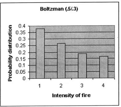
6.2 Effects of fire configuration on optimal solutions . . . . 6.3 Parameter tuning in the Boltzman distributions . . . . 6.4 Comparison of Approximate, Decoupled and Fully Collaborative

6.5 Effects of vision in the fully collaborative algorithm . . . .

6.6 Travel Time of Agents in Constrained Collaborative algorithm

6.7 Effectiveness of the Constrained Collaborative algorithm . . . .

61 . . . . 6 5 . . . . 6 7 . . . . 7 2 . . . 7 4 . . . 7 8 . . . . 8 0 85 . . . . 85 . . . . 88 . . . 93 algorithms . . . . . 96 . . . 104 . . . 107 . . . 108 . 46 . 46 54 56 57 . 58

6.8 Effects of vision range on the constrained collaborative algorithm . . . 111

6.9 Effects of non-line-of-sight communications on the constrained collaborative algorithm112

6.10 Effects of non-constant vision on the constrained collaborative algorithm . . . 113 6.11 Damage caused as a function of time . . . 115

7 Summary and Interpretation of Results 121

8 Future work 125

9 Appendix A - Markov Decision Processes 127

List of Figures

3-1 The Simulator display . . . ... ..2

Illustration of sample transportation problem Reduction in the number of agents considered Cost/Supply/Demand table ("Cost Table") . A sample cell . . . .

P ath . . . .

A sample cycle . . . . .. . . . .

Another sample cycle. . . . .. . . . . . A tree of cells . . . .. . . . . . A spanning tree of cells . . . .. . . .

Beginning the greedy allocation. . . .. . . .

After two allocations . . . . After three allocations .. . . . . The final allocation. . . . . Psuedocode for the greedy allocation...

. . . . . 30 . . . . . 32 . . . . . 32 . . . . 3 3 . . . . 3 4 . . . . 3 4 . . . . 3 5 . . . . 3 5 . . . . 3 6 . . . 3 7 . . . . 3 7 . . . . 3 8

4-15 Labelling an additional cell as basic with value zero . . . . 4-16 A cycle formed from a cell (S2, Dl) with negative reduced cost . . . .

. . . . 39 . . . . 39 . . . . 40 42 4-1 4-2 4-3 4-4 4-5 4-6 4-7 4-8 4-9 4-10 4-11 4-12 4-13 4-14 26

4-17 An improved solution.

4-18 Psuedocode for handling a negative cost cycle .

A possible cycle . . . . A cycle with fewer cells . . . .

One cell matched to two dimensions

(S3, D2) matched to its column . . . (S1, D3) is unmatched . . . . A path from X to Z . . . . A cycle in m+n cells . . . .

Two trees joined by a single cell . . .

A cycle formed within a tree .

4-28 A network flow problem derived from

Pseudocode for the typical value iteration method .

Pseudocode for the improved value iteration method

A linear probability distribution . . . . A Boltzman distribution with C1 = .3 and C2 = .3 A boltzman distribution with C1 = .3 and C2 = .5

A Boltzman distribution with C1 = .5 and C2 = .3

Area visible to an agent . . . . Range of communication for an agent . . . .

. ... 44 4-19 4-20 4-21 4-22 4-23 4-24 4-25 4-26 4-27 . . . 6 9 . . . 7 1 . . . 7 5 . . . 7 6 . . . 7 6 . . . 7 7 . . . . 7 9 . . . . 8 2

Differences between the approximation and optimal algorithms The "Small" fire configuration . . . . The "Mix" fire configuration . . . .

87 89 90 . . . . 4 5 . . . . 4 5 . . . 4 7 . . . 4 7 . . . 4 8 . . . 4 9 . . . 4 9 . . . 5 0 . . . . 5 1 a cost table . . . . 55 5-1 5-2 5-3 5-4 5-5 5-6 5-7 5-8 6-1 6-2 6-3 . . . 43

6-4 The "Far" fire configuration . . . 90

6-5 Comparison of algorithms in ten-fire, cost free problems. . . . . 97

6-6 Comparison of algorithms in fifteen-fire, cost free problems. . . . . 98

6-7 Damage relative to approximate algorithm in ten-fire, cost free problems. . . . . 99

6-8 Damage relative to approximate algorithm in fifteen-fire, cost free problems. . . . . . 99

6-9 Comparison of algorithms in ten-fire, travel-cost problems. . . . 102

6-10 Comparison of algorithms in fifteen-fire, travel-cost problems. . . . 102

6-11 Damage relative to approximate algorithm in ten-fire, travel cost problems. . . . 103

6-12 Damage relative to approximate algorithm in fifteen-fire, travel cost problems. . . . . 103

6-13 Factors controlling agent vision . . . 104

6-14 Effectiveness of agents with various vision ranges. . . . 106

6-15 Fully collaborative and constrained collaborative algorithm for ten-fire problem . . . 109

6-16 Fully collaborative and constrained collaborative algorithm for fifteen-fire problem . 110 6-17 Effects of vision parameters on constrained collaborative algorithm . . . 112

6-18 Effects of non-constant vision on constrained collaborative algorithm . . . 115

6-19 Damaged caused as a function of time for 4 fire, 7 agent problems . . . 116

6-20 Damaged caused as a function of time for 10 fire, 15 agent problems . . . 117 6-21 Damaged caused as a function of time during a constrained collaborative problem . 119

List of Tables

2.1 Fire M odels . . . . 23

3.1 Probability of fire growth . . . . 27

3.2 Hybrid Fire M odel . . . . 27

5.1 Damage caused to the city during each of the four scenarios . . . . 62

5.2 Algorithms to be Compared . . . . 64

6.1 Comparison of optimal and approximation algorithms on cost-free problems . . . . . 85

6.2 Effectiveness of approximate travel-cost algorithm . . . . 86

6.3 States in which the Approximation and Optimal algorithms differed . . . . 88

6.4 Initial intensities of various fire configurations . . . . 89

6.5 Effects of distance on optimal travel-cost algorithm effectiveness . . . . 91

6.6 Affects of distance on approximate travel-cost algorithm effectiveness . . . . 93

6.7 C1 and C2 values in the Boltzman Distribution for the cost-free decoupled algorithm 94 6.8 C1 and C2 values in the Boltzman Distribution for the cost-free, fully collaborative algorithm . . . 94

6.10 C1 and C2 values in the Boltzman Distribution for the travel-cost, fully collaborative

algorithm . . . . 95

6.11 Algorithm results for cost free, ten-fire problems . . . . 96

6.12 Algorithm results for cost free, fifteen-fire problems . . . . 97

6.13 Algorithm results for travel-cost ten-fire problems . . . 101

6.14 Algorithm results for travel-cost fifteen-fire problems . . . 101

6.15 Effectiveness of various vision parameters . . . 105

6.16 Time spent traversing the city in the constrained collaborative problem . . . 107

6.17 Results (in damage points) of the constrained collaborative algorithm on ten-fire problem s . . . 108

6.18 Results (in damage points) of the constrained collaborative algorithms on fifteen-fire problem s . . . 108

6.19 Effectiveness of vision in constrained collaborative algorithm . . . 111

6.20 Effectiveness of communication despite lack of line-of-sight . . . 113

Chapter 1

Introduction

Multi-agent collaboration, in which multiple entities cooperate to accomplish a shared goal, can be found throughout life. Research into automating such collaboration has targeted everything from soccer [11] to industry [6]. However, finding the optimal behavior for each agent in a group is a difficult task.

Constructing an optimal set of behaviors for every entity requires that every agent know the state of each of its peers and attempt to predict what actions they will take. This information must then be factored into the agents' decision making process. Suboptimal solutions, though more tractable, are of questionable value unless their degree of suboptimality is well characterized. This research identifies and quantifies the effects of various factors on the ability of a group of simulated fire fighting agents to extinguish a set of fires throughout a city. The following paragraphs discuss optimal and suboptimal approaches to multi-agent collaboration, the algorithms and comparison methods used in this work and the fire fighting domain these algorithms were tested in.

There are two common approaches to this problem, both of which use centralized planning. One approach is to assign optimal behaviors to each agent a priori [23], allowing each agent to carry out its plan independently of the other agents. Issuing a priori commands requires detailed

knowledge of the problem before a solution can be constructed. In addition, this style of multi-agent collaboration is extremely inflexible; if circumstances deviate at all from their expected state the entire plan may become useless. Another approach that has been taken towards multi-agent collaboration is to have some form of central coordination that issues commands to every agent in the group as the situation unfolds[5], requiring constant communication between group members.

If a central coordination mechanism with global knowledge issues commands to and receives

information from every agent then the problem can be reduced to finding the optimal set of orders that the central coordinator should issue, given the state of the world. In this type of problem there is no real collaboration; only one entity makes any decisions. One method for calculating the optimal set of orders to be issued in any given world-state is through the use of Markov decision processes [10, 17] (MDPs). Appendix A provides a brief description of MDPs and the value iteration

algorithms used herein.

Despite the attractiveness of optimal solutions, there are several drawbacks to the centralized approach. Centralized planning requires perfect communication between the coordinating entity and all of the agents and is hampered by damage to the coordinating agent, which is a single point of failure. In addition, development of an optimal multi-agent policy typically requires detailed knowledge of the problem as a whole, which is likely to be infeasible for realisitically complex problems.

Since agents in an urban environment typically do not have global knowledge of the entire city, and often have limited communications with each other or with a central coordinator. This re-search examines the effects of various factors on agent performance. These factors are the presence or absence of global knowledge, the presence or absence of central coordination, variations in the communication and vision range and the speed at which agents travel around the city. Five algo-rithms were developed to support review of the various factors. An optimal algorithm was designed

and implemented. This algorithm relies on global knowledge and perfect communications and is very computationally intensive for all but the most trivial problems. A near-optimal approximation algorithm was used in order to solve problems involving larger numbers of agents and fires. In order to examine the effects of central coordination, a third algorithm was developed that did not rely on central coordination but still allowed the agents global knowledge of the city. A fourth algorithm was also designed that required neither global knowledge nor central coordination; comparing this algorithm to the previous one helps to demonstrate the effects of global knowledge on agent ef-fectiveness. Finally, a fifth algorithm was developed which did not rely on global knowledge or coordination and also imposed more realistic constraints on the rate at which agents could travel around the city. The effects of these constraints are discussed as well.

Since solving Markov decision problems is computationally intensive, the size of tractable prob-lems that can be solved optimally is prohibitively small. As a result, a three-level comparison was performed between the optimal solutions (for problems of small size), near-optimal solutions created using an approximation algorithm discussed below and the algorithms discussed in this work.

For comparison purposes, all of the algorithms were run in situations for which an optimal, centralized solution could be constructed. In addition, the algorithms were run in situations for which construction of an optimal solution is computationally intractable; these iterations and their results are discussed in Chapter 6.

The agents' performance increased quickly as their range of knowledge increased, although it plateaued after a certain range. Agents with global knowledge but no centralized control performed nearly as well as centrally controlled agents with global knowledge. The results for problems of various sizes are discussed in Chapter 6.

This algorithm has been adapted for use in this thesis and compared with the results of the optimal algorithm. The results are discussed in Chapter 6. This approximation is used as a baseline for judging the results of this project on problems which are too large to solve optimally using MDPs. This work deals with the fire fighting domain. Although prior research' has already developed algorithms for use in this domain [2, 5, 12], these algorithms rely on either centralized control or knowledge of the entire world. This project uses a simple simulation that models a few city blocks; the simulator models the increase in intensity of the fires throughout the city as well as the efforts of the fire fighters to extinguish them. This simulator is used to compare the effectiveness of the various distributed algorithms, the near-optimal approximation and the optimal MDP solution. The RoboCup Rescue project [12] has developed a similar simulator, but it is unsuitable for this research for reasons that will be detailed in Chapter 6.

The remainder of this thesis is laid out as follows: Chapter 2 describes prior research done in this field including the requirements for the creation of an optimal solution and previous work aimed at developing near optimal solutions that bypass these requirements. It also further describes the goals and motivations behind this work. Chapter 3 discusses the simulator that is used in this research as well as the particulars of how fires and fire fighters are modeled. Chapter 4 discusses the stepping stone algorithm, which is used to calculate the cost of moving a set of agents between fires. Chapter 5 discusses the algorithms implemented during this research and the situations in which they are applicable. Chapter 6 discusses the tests performed on the various algorithms and the results that were obtained. Chapter 7 summarizes the thesis and presents an interpretation of the results as a whole. Chapter 8 discusses some of the possible future extensions to this work. Appendix A discussed the Markov Decision Problems used to model the simulation and the value iteration algorithm used to provide optimal agent behavior.

Chapter 2

Related Work in Fire Suppression

One application for which multi-agent collaboration is currently being explored is cooperative fire-fighting [2, 5, 12], where simulated fire fighting agents work together to either contain [5] or extinguish [2, 12] fires. The following sections describe related work in modeling fire spread and fire suppression.

2.1

Previous Fire Models

Much of the previous work in fire simulation has focused on creating a realistic fire model that is simple enough computationally to be used in a simulation involving many fires spreading over a wide area of land. Several of these approaches are documented below.

2.1.1 A Simple Grid of Cells

One widely used approach is to model the fire as a lattice of cells. The cells are either on fire or not (there is no intensity) and burn through their fuel supply at a predetermined rate. Individual cells have their own fuel supply. At every time step there is some probability that the fire will spread to nearby cells based on factors such as wind, hill gradient, etc. This model treats each cell

as a separate fire.

Previous work using this model has represented fire suppression in various ways. Cohen has the fire-fighting agents contain the fire and wait for it to run out of fuel [5]. Since Cohen was simulating large scale forest fires and the agents were often far apart from each other, he relied on a centralized "fire boss" to coordinate the agents when they were far apart.

Andrade models fire suppression efforts by reducing the amount of fuel that a particular cell has, thus decreasing the time before it burns out [2]. Andrade's model requires agents to reduce the fuel for each cell individually. Andrade modeled fire fighting in individual rooms on a ship. Thus, each agent had complete knowledge of the room it was in, including the location of each of the fires.

2.1.2 Rothermel's Work

Many fire simulations (e.g., [8, 15]) which model the spread of fires in the wilderness are derived from work developed by Rothermel in 1972 [18]. These systems model a fire as a collection of cells, which spreads by igniting nearby (non-burning) cells. Unlike the simple grid of cells discussed previously, individual cells can have different intensities which affect how likely the fire is to spread to neighboring cells. The intensity of a cell is based on the type of fuel being burned and is not time dependent. Each cell is described by its fuel type, amount of fuel, current state (i.e., on fire or not), susceptibility to being lit on fire by other fires and many other factors. Additionally there are global factors such as terrain, wind conditions and moisture in the air that affect all of the cells. Fire suppression is not typically studied using this type of simulation; these models are generally used to study how a fire will spread unchecked through a forest [7].

2.1.3

The RoboCup Rescue Simulator

The RoboCup Rescue project [12] has developed a simulation that will allow multiple agents to cooperatively fight fires with only local knowledge and limited communications. This promises to be a very useful environment for future research. However, the current efforts of the RoboCup Rescue development team are focused on improving the simulator, rather than designing or implementing the agents' strategies, making it less applicable to this thesis. Since the RoboCup Rescue project has just begun [20], the algorithms used in the project are not very sophisticated. For example, each agent simply heads towards the closest fire, regardless of how many other agents are heading towards or already at that same fire.

Several characteristics of the current implementation of the RoboCup Rescue simulator make it unsuitable for the current research. They include the inability to reset the simulator state, the lack of distance and line-of-sight constraints on agent vision and agent communication, and the need for a more realistic fire fighting model.

The fire models discussed in this chapter are summarized in table 2.1.

Simple Grid Rothermel's Model RoboCup Rescue

Same intensity across fire Yes No No

Intensity changes over time No No Yes

Fires consume fuel Yes Yes Yes

Used to model fire suppression Yes No Yes

Chapter 3

The Simulator and Fire Model

This chapter discusses the simulator used in this research (in section 3.1) and describes the way that fire and fire suppression were modeled (in section 3.2). Each of the agents in the simulator determines and executes its plan of action.

3.1

The Simulator Engine

The simulator used in this research is a simple Java program that models fires and fire fighting agents within a few city blocks. The city is represented as a grid of nodes of three types ("road",

"fire" or "building"). "Building" nodes can catch on fire. Fires that are extinguished are still treated as "fire" nodes, but with zero intensity. Each fire has its own intensity, discussed in section

3.2. The simulator models constraints such as vision and communications bounded by line-of-sight

and distance.

The simulator consists of a single main loop that first updates all of the fires (increasing or decreasing their intensity if appropriate), then provides the agents with the information available to them (about the entire world if the scenario allows global knowledge, otherwise only about the

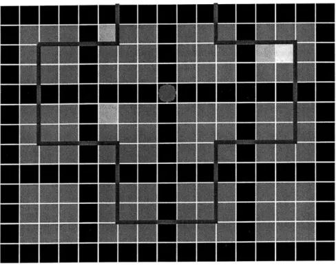
applicable portions of the world) and runs each agent's decision making routine. As part of the decision making process, each agent decides which fire to fight or, if central coordination is present, is assigned to a fire. Figure 3-1 shows the simulator display. The black squares forming a grid through the picture indicate roads. The magenta circle at the intersection.is a fire fighting agent. The two light gray squares above and to the right of the agent are low intensity fires. The other squares represent unburned ground.

U EE.EEENEE U

Figure 3-1: The Simulator display

3.2

The Hybrid Fire Model

This section describes the model used to represent fires in this research. This hybrid model retains many of the characteristics of the previously discussed fire models, but is simplified for use

with MDPs.

Each fire has one of five intensity levels; as the fire reaches each new intensity level it does more damage. For example, a level one fire might scorch the paint off walls, while a level four fire might cause total destruction. Level zero is used to denote fires that have been extinguished. There is an a priori probability that a fire at one particular level of intensity will jump to the next level

of intensity; this probability is based only on the fire's current level. The probability of the fire increasing in intensity goes up as the fire intensity increases. For example, level-three fires have a

60% chance of becoming level-four fires in the next time step whereas level one fires have only a 15% chance of becoming level-two fires in the next time step. Table 3.1 lists the odds of fires at

various intensities increasing to the next level.

Intensity of Fire Probability of Increase

0

I

1 .15

2 .35

3 .6

4 0 (Maximum intensity)

Table 3.1: Probability of fire growth

There is also some probability that a fire will decrease by one level of intensity. This probability is a function of the number of fire fighters fighting the fire and the current intensity of the fire. The effectiveness of each additional fire fighter decreases as the number of fire fighters assigned to the fire increases. For example, having one fire fighter fight a particular fire might provide a 10% chance that the fire will decrease in intensity while having two fire fighters might only provide a

17% chance that fire's intensity will decrease. Table 3.2 summarizes the properties of the hybrid

fire model.

Hybrid Fire Model Same intensity across fire Yes

Intensity changes over time Yes

Fires consume fuel No

Used to model fire suppression Yes

Table 3.2: Hybrid Fire Model

useful to this project. Fires that are not extinguished will eventually increase in intensity and, more importantly, will continue to increase in intensity at a faster and faster rate. This forces the agents to attempt to fight every fire they have a realistic chance of stopping, because fires that grow past a certain threshold will be very hard to control. In addition, the decreasing effectiveness of additional fire-fighters means that the agents need to spread out their efforts for maximum gain while still concentrating their efforts enough to fight fires that are on the verge of becoming uncontrollable.

It is very important that the fire model be kept as simple as possible in order to increase the size of the problems that are optimally solvable via MDPs. As a basis for comparison, it took a Sun UltraSparc 20 with a 333 MHz processor one hour to solve the MDP corresponding to four fires, each using the hybrid fire model, and seven fire fighting agents. It took the same computer six hours to solve a two fire, four agent problem when the problem used the RoboCup Rescue fire model because the RoboCup Rescue fire model allows the same fire to have different intensities at different points across its surface and also keeps track of the fuel consumption of each fire.

Chapter 4

The cost of moving agents during a

single action

In this research, the "actions" evaluated by a Markov Decision Process (MDP) are simply assignments of agents to fires. At any given time the agents are already at various locations. Thus, the reward for a given action has to take into account the cost of moving the agents from their current locations to the ones designated by the MDP. This chapter describes an algorithm used by the simulator to quickly compute these costs.

For example, consider a situation with four fires (A, B, C, D) and two agents (a, b), where agent "a" is at fire "A" and agent "b" is at fire "B". The cost to assign an agent to "C" and an

agent to "D" is the minimum of C(A, C) + C(B, D) and C(A, D) + C(B, C), where C(X, Y) is the

cost of moving an agent from location X to location Y. Figure 4-1 illustrates this problem.

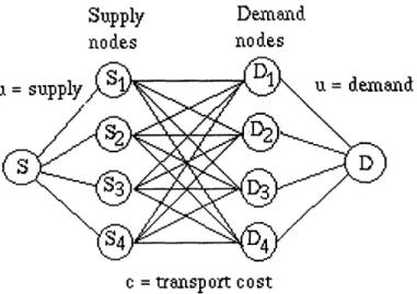
This type of problem is a transportation problem [21]; it is a special case of a weighted bipartite matching problem which is in turn a special case of a min-cost flow problem. For computational efficiency reasons, the algorithm implemented in this research is Charnes and Cooper's "stepping

Moving an agent from A to C and from B to D

A

B

C

D

Moving an agent from A to D and from B to C

A

B

G

GD

1"

C)

D

Figure 4-1: Illustration of sample transportation problem

stone" algorithm [4], which is described in detail below.

The stepping stone algorithm is based on the network simplex method, and thus has a similar running time. Although there is no known method that will make the simplex method run in poly-nomial time [19], in practice the network simplex method, and thus the stepping stone algorithm, run very quickly.

Since the transportation problem is a special case of a min-cost flow problem, it is possible to use min-cost flow algorithms to solve it. However, an average problem uses very few iterations of the stepping stone algorithm and thus runs considerably faster than most min-cost flow algorithms. For example, if the number of nodes in a graph is n and the number of edges if m, the running time of the algorithm described by Galil [9] grows with O(n2_{(m + n log n) log n). By comparison,} a single iteration of the stepping stone algorithm grows in O(m + n)2

time. The stepping stone algorithm is used to calculate the cost of moving a set of agents from their current locations to a

set of new locations. This cost is then factored into the instantaneous reward associated with a given action in the MDP.

4.1

Overview of the stepping stone algorithm

The stepping stone algorithm minimizes the cost of transporting agents from m sources to n destinations along mn direct routes from source to destination. Each path from a source to a destination has a cost associated with it. That cost is applied to each agent that travels along the route. The algorithm is based on the simplex method of solving linear programming problems; it begins by creating a feasible solution to the problem and then refining that solution until an optimal solution is reached.

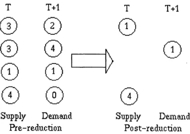
Before the stepping stone algorithm is called, the simulator determines which locations have more agents than are needed and which locations require additional agents. The simulator assumes that each fire either "supplies" agents or "receives" agents, but not both. Since the travel cost is linearly proportional to the distance traveled, it is always possible to construct an optimal solution that does not require an agent to leave a location and a different agent to enter that location. Al-though this isn't neccessary, it speeds up the calculation of the final solution considerably because it means that the stepping stone algorithm only needs to consider the number of agents either "sup-plied" or "received" at each fire, rather than the total number of agents. Figure 4-2 demonstrates one such reduction. The pre-reduction circles indicate the number of agents at each location for a given time and the post-reduction circles indicate only the agents that the stepping stone algorithm will consider.

The stepping stone algorithm begins by generating a table correlating the various costs, supplies and demands. Figure 4-3 shows a sample table. Each row represents a source location; the number

T

T+1

Supply

Demand

Pre-reduction

T

0

T+1

Supply

Demand

Po st-reduction

Figure 4-2: Reduction in the number of agents considered

of available agents is shown in parentheses next to the location name. Each column represents a destination and lists its total demand in parentheses.

Destination(Demand)

Source

D1(4)

D2(2)

(Supply)

S1(2)

S2(5)

S3(6)

D3(1)

D4(6)

Figure 4-3: Cost/Supply/Demand table ("Cost Table")

For example, the cell (S1, D2) in figure 4-3 shows the cost of transferring an agent from S1 to D2 (the cost is 1) and the number of agents being sent from S1 to D2 (2 agents are being moved). In order for a solution to be feasible, the values in each row must add up to the total supply available at that location and the values in each column must add up to the total demand

2

1

3

4

3

7

5

8

at that location. For example, (S2, D3) + (S2, D4) = S2S, = 5. Figure 4-3 shows a sample

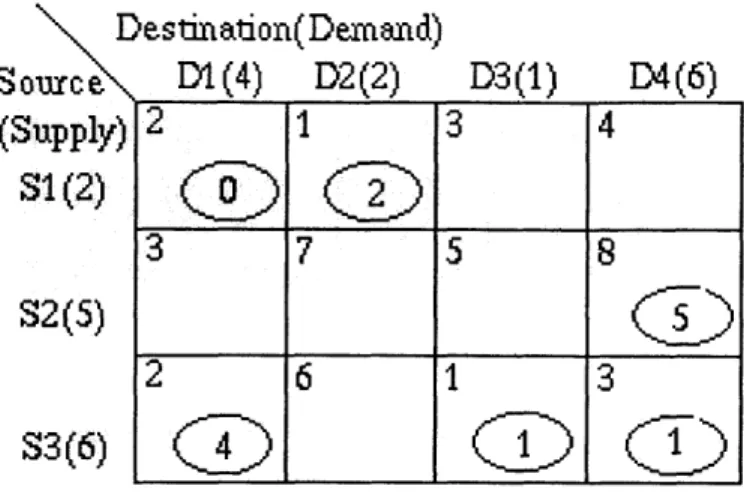
table with costs, supplies, demands and cell values. Such tables will be referred to as "cost tables." Sources with no surplus agents and destinations requiring no additional agents are dropped from the table. The cost of transporting an agent from a source to a destination (the cost of the cell) is indicated in the upper left corner of the corresponding cell. The number of agents being transported along that route (the value of the cell) is also shown. For the purposes of clarity, cells that have not been marked as "basic" (see below) do not have their value displayed in any of tables in this section; each of these "non-basic" cells has a value of zero. Figure 4-4 shows a sample cell with cost 3 and value 4; the cell is marked as "basic".

Figure 4-4: A sample cell

A "path" of cells is a sequence of cells in the cost table. The cells in a path do not have to be

adjacent in the cost table but each cell must share either a row or column with the both previous and next cells along the path. Figure 4-5 shows a path through various cells of the cost table. The

path starts at (S1, Dl) and includes (S3, Dl), (S3, D3), (S2, D3), (S2, D4) and (S3, D4). Note that the path does not include (S2, D1) or (S3, D2). A path cannot include the same cell more than once except when it forms a cycle, as noted below. Thus (S2, DI), (S2, D2), (S2, D1), (S3,

DI) is not a valid path. In all diagrams in this section, the arrow heads will denote cells actually

included in the path.

A "cycle" is a path of cells that starts and ends at the same cell. Cycles "originate" at the first

Destination(Demand)

D1(4)

D2(2)

D3(1)

D4(6)

Source

(Supply

S1(2)

S2(5)

S3(6)

Source

(Supply)

31(2)

S2(5)

S3(6)

Figure 4-6: A sample cycle

)2

1

3

4

3

7

5

8

2

6

1

3

Destination(Demand)

DI1(4)

D2(2)

D3(1)

D4(6)

2

1

3

4

7

5

8

2

6

1

3

Source

(Supply)

S1(2)

S2(5)

S3(6)

)estination(Demand)

D1(4)

D2(2)

D3(1)

D4(6)

2

1

3

4

3

7

5

2

6

1

3

Figure 4-7: Another sample cycle

A set of "connected" cells is an unordered set of cells such that there is a path between any two

cells in the set made up entirely of cells within the set.

A "tree" of cells is an set of connected cells such that there are no cycles made up of cells in

the tree. Figure 4-8 shows a tree of cells. The tree contains the cells (S2, D1), (Si, D3), (S2, D3), (S3, D3), (S3, D4). For example, (S2, Dl), (S2, D3), (S3, D3) is a path between (S2, D1) and (S3,

D3) composed entirely of cells in the tree.

OIC

Source

(Supply)

SI(2)

S2(5)

S3(6)

)estination(Demand)

D1(4)

D2(2)

D3(1)

D4(6)

Figure 4-8: A tree of cells

A "spanning tree" is a tree which contains a cell in every row and every column of the cost

2

1

3

4

3

7

5

-2

613

table. Figure 4-9 shows a spanning tree of cells.

D

S ouxc

e

(Supply)

S1(2)

S2(5)

S3(6)

estination(Demand)

D1(4)

D2(2)

D3(1)

D4(6)

2

1

3

4

3

7

5

8

2

6

1

3

Figure 4-9: A spanning tree of cells

4.1.1 Step 1 - Initial Solution

The stepping stone algorithm uses a greedy approach to create the initial feasible solution. The cell with the lowest cost among those whose supply and demand constraints are both unfulfilled (greater than zero) is chosen and enough agents are assigned to that cell to fulfill the smaller of the two constraints on that cell. If two cells with unfulfilled constraints have the same cost than either of them may be used. As agents are assigned to each cell the remaining supply and demand totals on that cell are reduced. This process is repeated until every supply and demand constraint has been satisfied; proof that all of the constraints will be satisfied is given below. Figures 4-10, 4-11, 4-12 and 4-13 show this process occuring. The grey bars indicate supply and/or demand constraints that have already been fulfilled and the grey numbers represent the value of the reduced constraints.

Note in figure 4-11 that the S3 constraint has been reduced to 5, but not yet fulfilled.

In figure 4-12, cell (S3, Dl) was chosen because it has the lowest cost among the cells with both constraints unfulfilled. Although cell (S3, D3) has lower cost, one of its constraints has already

Destination(Demand)

Source

1(4)

D2(?f

A

(Supply)

S2(5)

S3(6)

Figure 4-10: Beginning the greedy allocation

Destination(Demand)

Source

D1(4)

D2Qj

(

S2(5)

S3

D3f

0 D4(6)

Figure 4-11: After two allocations

D3(1)

D4(6)

2

1

3

4

3

7

5

2

6

1

3

24

2

351

4

_I <9±1

(Supply)

2

6

I

3

been fulfilled.

Destination(Demand)

Source

D14 ( )D2

)j

,D3fJt()

D4(6)

(Supply) 2

1

Sp

3

7

5

8

S2(5)

216

1

3

Figure 4-12: After three allocations

Assigning a value to a cell must fulfill at least one constraint, and the last cell must fullfill two constraints since the total supply and total demand are the same. Since the allocation finishes when all of the constraints are fulfilled, the greedy algorithm requires filling at most m + n - 1 possible

cells where m is the number of sources and n is the number of destinations. In the above example, the first allocation fulfilled two constraints (both the S1 and D2 constraints) so only m + n - 2 cells were required. Pseudocode for the greedy allocation can be found in figure 4-14.

4.1.2 Step 2 - Basic Cells

The cells chosen in the previous step are marked as "basic" cells. Since each basic cell is chosen on the condition that both its supply and demand constraints are unfulfilled, the basic cells will not form a cycle. If there are less than m

+

until there are m + n - 1 basic cells. The additional cells are chosen in such a way that there are

no cycles among the basic cells. Proof that these additional cells always exist, as well as a method to pick them, is discussed below.

Destination(Demand)

Source

DIS(4)

D2 f'f0

(Supply

SI)

52 (5

2

3

4

L

.

.Z

...

L _

...

...

_ _

...

---..

SI24

y3

Figure 4-13: The final allocation

notDone = true

//

while notDone

do notDone = false

min-i = 0

min-j = 0

//

for i = 0 to length[columns]

do for

j

do if table[i][j].cost < table[min-i][min-j].cost and columns[i].constraint > 0 and rowsj].constraint > 0 then min-i = i min-j = j notDone = true if notDone

//

then table [i] [].value = minimum (columns [i].constraint, rows [j]. constraint) columns [i]. constraint = columns [i].constraint - table[i][j).value rows[j].constraint = rows[j].constraint - table[i] [j].value

Figure 4-14: Psuedocode for the greedy allocation

10

20

)~f

D3

(0)Dffo()

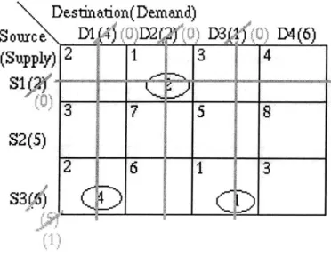
Figure 4-15 shows cell (S1, Dl) being labeled as basic. The value of the cell is still zero.

estination(Demand)

Dl(4)

D2(2)

D3(1)

D4(6)

Figure 4-15: Labelling an additional cell as basic with value zero

4.1.3 Step 3 - Dual Costs

Improving the initial solution requires calculating the "dual" costs for every cell in the cost table. As in the Network Simplex Method, the dual cost of a cell reflects the potential change in the value of a solution if that cell were included. Including cells with a negative dual cost would improve the solution while including cells with a positive dual cost would degrade the solution. Cells already included in the solution have a dual cost of zero, as do cells whos inclusion into the solution would not change the value of the solution.

Before the dual costs for the cost table cells can be calculated, the "dual values" for the various rows and columns must first be computed. These values will be used to compute the dual costs of the individual cells, but have no meaning on their own. Calculating the dual values for the various rows and columns can be done by using the cost equations for the basic cells. The cost equations read:

D

Souc

e

(Supply)

S1(2)

S2(5)

S3(6)

2

1

3

4

3

7

5

8

C)

2

6

1

3

C)

(DC

U, + V =QCj (4.1)

Here Cij is the given cost for the basic cell, Ui is the dual value for row i and Vj is the dual value for column j. Since there are m + n - 1 dual equations (one for each of the basic cells) and

m +

n

Once the dual costs for the rows and columns are calculated, the reduced cost for non-basic cell (i,

j)

RC~j

(Ut + 1/i)

The reduced cost for a non-basic cell represents the change in the value of the solution which results from making cell ij basic and making adjustments around the cycle of basic cells thus created in the solution. There were originally m + n - 1 basic cells, marking an additional cell as basic

creates m + n basic cells. Proof that any collection of m + n cells must include a cycle can be found below.

If all of the reduced costs for non-basic cells are non-negative then the solution is optimal;

including additional cells in the solution will not improve the solution at all. Proof of this is discussed below, under the heading "Optimality Conditions" in the "Proof of Correctness" section.

If one of the non-basic cells has a negative reduced cost, it can be added into the solution in the

following manner.

4.1.4 Step 4 - Negative Reduced Cost Cycles

Consider a cycle of cells that involves a non-basic cell with a negative reduced cost and various basic cells. The m + n - 1 basic cells were chosen such that they do not form a cycle. Since it is

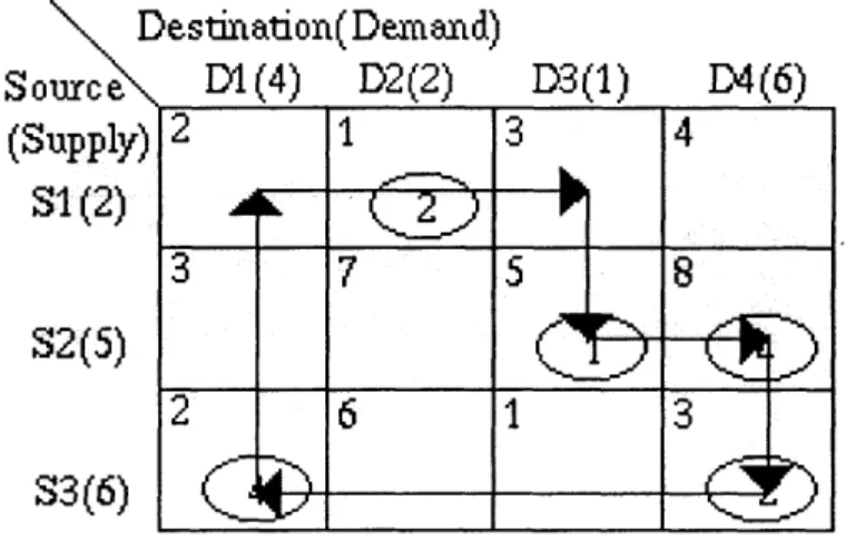
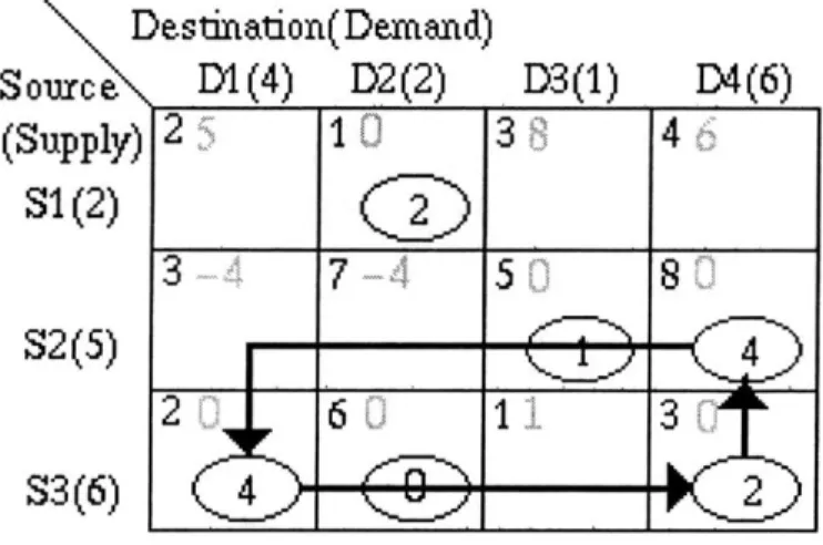
impossible to pick m + n cells such that there are no cycles (see section 4. 4.1.1) it must be possible to choose such a cycle. This cycle is refered to as a "negative cost cycle." Figure 4-16 shows the cycle formed from basic cells and a single cell with a negative reduced cost. Note that the cell values used in figure 4-16 were not generated using the greedy algorithm but do represent a feasible solution to the transportation problem. Numbers in gray represent reduced values. Cell (S3, D2) has been marked as basic (with value zero) in order to ensure that there are m + n - 1 basic cells.

Destination(Demand)

Source

D1(4)

D2(2)

D3(1)

D4(6)

(Supply)

S1(2)

S2(5)

S3(6)

Figure 4-16: A cycle formed from a cell (S2, D1) with negative reduced cost

The first cell in the cycle (the cell with negative reduced cost; (S2, D1) in the example) is labeled "positive." The other cells are alternately labeled "positive" or "negative." The "flow" around this cycle is defined as the value of the smallest "negative" cell. In figure 4-16 the flow would have value 4.

The flow around this negative cost cycle is then subtracted from every negative cell and added to every positive cell. The first positive cell is then labeled basic, and one of the negative cell which now has zero value is labeled non-basic. Figure 4-17 shows the cost table after the flow around the cycle has been added to every positive cell and subtracted from every positive cell; cell (S2, D1) has been made basic and cell (S3, D1) has been made non-basic. The dual values for each row

2-

10

38

46

3.,

7-4

50

80

4

2'

.0

1

3 I J

and column are recomputed using the new set of basic cells and the dual costs for each cell are recomputed using the new dual values. The process is then repeated until none of the non-basic cells have a negative reduced cost. Note that the combined cost of the four cells in the cycle in figure 4-16 is C(S2, D1)V(S2, D1) + C(S3, D1)V(S3, D1) + C(S2, D4)V(S2, D4) + C(S3, D4)V(S3, D4) = 3. 0 + 2 -4+ 3 .2+8. 4 = 46 where C(i, j) is the cost of cell (i,

j)

j).

+

Destination(Demand)

Source

D1(4)

D2(2)

D3(1)

D4(6)

(supply)

S1(2)

S2(5)

S3(6)

Figure 4-17: An improved solution.

The search procedure mentioned on line 2 returns an array of the cells found in the cycle created

by the basic cells and the negative reduced cost cell. Proof that this cycle can always be found is

given below; a simple depth-first search algorithm can be used to find the particular cells. If any three or more cells in the cycle all share the same row or the same column then only the first and last cells in that row or column are included in the cycle. Figures 4-19 and 4-20 demonstrate this

2

1

3

4

3-4

7-4

5

0

4

_0.

0

6 0

11

3

//

cycle = search(start-cell)

//

min-negative = positive-infinity

min-index = -1

for i = 0 to length[cycle]

do if i mod 2 == 0 and

/1

min-negative < cycle[i.value then min-negative = cycle[i].value

min-index = i

/

start-cell.value = start-cell.value + min-negative for i = 0 to length[cycle]

do if i mod 2 == 0

then cycle[i].value = cycle[i].value - min-negative else cycle[i].value cycle[i].value + min-negative

//

start-cell.basic = true

//

cycle[min-index].basic = false

Figure 4-18: Psuedocode for handling a negative cost cycle

10

Destination(Demand)

Source

D1(4)

D2(2)

(Supply)

S1(2)

S2(5)

S3(6)

D

Source

(Supply)

S1(2)

S2(5)

S3(6)

D3(1)

D4(6)

2

1

3

4

3

7 (+

5

8

2

6

1

3

Figure 4-19: A possible cycle

estination(Demand)

D1(4)

D2(2)

D3(1)

D4(6)

2

1

3

4

3

7

5

8

2

6

1

3

Figure 4-20: A cycle with fewer cells

Removing cells in this fashion can never result in the negative-reduced cost cell (the non-basic cell) being removed, because doing so would form a cycle of only basic cells. The set of basic cells must be acyclic. Proof of this is given in below.

This process results in a feasible solution with lower total cost unless the flow around the negative cost cycle is zero, in which case the total cost will not change. If the flow is zero and another non-basic cell has a negative reduced cost then the same procedure is applied to it. If the

4.2

Proof of correctness of the stepping stone

algorithm

This proof is divided up into sections detailing various stages of the stepping stone algorithm. [4]

4.2.1 Constructing the initial solution

Theorem 1 At most m + n - 1 cells are chosen by the greedy allocation.

Each basic cell chosen during the greedy allocation is chosen such that it fulfills either the supply or demand constraint for its row or column. Since the sum of all of the supply constraints equals the sum of all of the demand constraints and the value of each basic cell is subtracted from both a supply and a demand constraint, the final basic cell must satisfy two constraints. Thus, there must be at most m + n - 1 cells.

Theorem 2 A set of m + n or more spanning cells must form a cycle.

A set of spanning cells includes a cell in every row and every column of the cost table. The

cells can be matched up with the rows and columns in a manner similar to that used to create only cell with negative reduced cost is in a cycle with zero flow then the solution is optimal.

If the flow was not zero (and the algorithm has not terminated) then the cells are labeled basic

or non-basic as appropriate and the algorithm is repeated. If more than one cell in the cycle has been reduced to zero flow only one of them is labeled non-basic.

This process continues until the reduced cost for each of the non-basic cells is non-negative. Proof that the algorithm eventually terminates and that it produces an optimal solution can be found below.

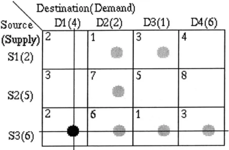
the initial greedy solution; one of the cells is matched up with both its row and column. Any cell who's column or row has been matched to a different cell can then be matched to its remaining, unmatched dimension. Figure 4-21 shows a set of m + n cells. Cell (S3, Dl) has been matched with both its row and its column.

Destination(Demand)

Sourc e

D1(4)

D2(2)

(Supply)

S1(2)

S2(5)

S3(6)

D3(1)

D4(6)

Figure 4-21: One cell matched to two dimensions

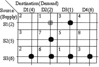
Figure 4-22 shows one of the cells in the

cell (S3, D2) matched with its column. set with only one unmatched dimension.

(S3, D2) was chosen because it was

Destination(Demand)

Source

1(4)

D2(2)

(supply)

SI(2)

S2(5)

S3(6)

Figure 4-22: (S3, D2) matched to its column

2

1

3

4

3

7

5

8

2

6

₃

2

13

4

3

758

2

IS

D3(1)

D4(6)

The first cell was matched with both its row and its column. Since there are m

+

Destinadon(Demand)

21

3

4

3

7

5

8

2

6

1

3

This cell is part of a cycle. Since X was not matched to its row, but its row was matched up with a cell, there must be another cell Y in the same row as X that was matched with the row X

is on. In figure 4-23, X is cell (S1, D2) and Y is cell (S1, D3).

Y was matched with either its column or with both its row and column. If Y was matched with only its row then that means that there must be another cell in the same column as Y that was matched with that column. This new cell, Y', is connected to X by the path Y'-> Y->X and is similarly matched with either just its column or with both its row and column. In figure 4-23,

cell (S3, D3) is Y'.

This path can be continued until it reaches Z, the cell which was originally matched against both its row and its column. In figure 4-23, Z is cell (S3, D1). Z was matched up with the row

that Y" is on, thus the path goes from (S1, D2) to (S1, D3) to (S3, D3) to (S3, D6). Figure 4-24

~Soure'

(SuppIy

S1(2)

S2(5)

shows the complete path.

Destination(Demand)

(Supply)

S1(2)

S2(5)

S3(6)

T4 (6)

Figure 4-24: A path from X to Z

A similar path can be constructed beginning with the cell in the same column as X. This path

can also be extended until it reaches Z. There are now two distinct paths connecting X to Z;

reversing the direction of one of these paths will form a cycle among the m

+

Destination(Demand)

Source

(supply)

S1(2)

S2(5)

S3(6)

Figure 4-25: A cycle in m+n cells

Thus, a set of m + n cells in a cost table must form a cycle.

2

i

3

4

3

7

5

8

2

6

13

2

3

4

3

7

L5

8