The design and field evaluation of a new dual pressure and temperature tapered probe

The Design and Field Evaluation of a New Dual Pressure and

Temperature Tapered Probe

by

Matthew G. Chartier

Bachelor of Science in Geology

New York State College at Oneonta, Oneonta, New York (2000)

SUBMITTED TO THE DEPARTMENT OF CIVIL AND ENVIRONMENTAL ENGINEERING IN PARTIAL FULFILLMENT OF THE REQUIREMENTS FOR THE

DEGREE OF

MASTER OF SCIENCE IN CIVIL AND ENVIRONMENTAL ENGINEERING AT THE

MASSACHUSETTS INSTITUTE OF TECHNOLOGY

June 2005

@ 2005 Massachusetts Institute of Technology All rights reserved

MASSACHUS9tTS INSTfTUT OF TECHNOLOGY

MAY

3 12005

LIBRARIES

-Department of Civil and Environmental Engineering May 23, 2005

Certified by

Principal Research Associate of Civil and

J.1p

-Professo rrdrew J. Whittle Chairman, Department Committee for Graduate Studies

The Design and Field Evaluation of a New Dual Pressure and Temperature Tapered Probe

by

Matthew G. Chartier

Submitted to the Department of Civil and Environmental Engineering on May 23, 2005 in partial fulfillment of the requirements for the degree of

Master of Science in Civil and Environmental Engineering

ABSTRACT

The T2P is a new penetration device that measures temperature at its tip and pore pressure at a point just above the tip and at a second location near the base of the probe shaft. The main purpose of the T2P, recently designed and fabricated at MIT, is to reduce the time required to accurately estimate in-situ pore pressures (u.) of marine sediments. This goal will be accomplished by using the two-point matching method (Whittle et al., 1997; 2001) to compare measured partial T2P dissipation records with theoretical dissipation curves, derived using the Strain Path Method (Baligh, 1985) and total or effective stress soil models.

A four-day field program was conducted at a test site in Newbury, Massachusetts to

evaluate the design and performance of the T2P. The field program was designed with the intention of performing a number of dissipation tests at a series of elevations within a deep deposit of Boston Blue Clay. Twenty-four hour operation of the data acquisition system allowed overnight dissipation data to be collected. Two boreholes were used to collect a total of eight pore pressure dissipation records, whose length ranged from 0.74 to 19.74 hours. It is not clear if any of the eight monitoring periods were of sufficient duration for full dissipation to occur; it is suspected that measurement periods longer than 20 hours are required to allow complete dissipation around the probe, which is in agreement with previous research (Varney, 1998).

The field test data was used to estimate uO at various locations within the clay, using the inverse time extrapolation method and the two-point matching method. It was found that inverse time extrapolation could be used to approximate uO within 10% accuracy from T2P tip data within an average monitoring time of 942 seconds; however, the two-point matching method consistently produced more accurate estimates of uO than inverse time extrapolation at similar dissipation times. In addition, soil hydraulic conductivity (k) was interpreted by comparing the measured dissipation data with theoretical curves, using the T50 matching method. The calculated

values of k closely matched values previously obtained through laboratory measurements. The T2P field test data is compared with piezoprobe and piezocone penetration and dissipation records, collected at a site in Saugus, Massauchusetts (Varney, 1998).

Recent modifications have been made to the T2P prototype since the 2004 field test, in preparation for an upcoming sea deployment. These modifications were based upon the field performance of the T2P prototype and design changes required for offshore operations.

Thesis Supervisor: Dr. John T. Germaine

ACKNOWLEDGMENTS

I am forever indebted to my wife, Christina, for keeping me sane during my time at MIT and for constantly believing in me. I could not have made it without her.

Of course, I could never repay my parents for all the love and support that they've given me over the years. This thesis is not big enough to contain all the reasons that I have to be thankful to them.

Special thanks to Dr. Lucy Jen for having more faith in me that I ever did myself, and for pushing me to achieve things that I never considered possible. She has been a great friend and an inspiration to me.

I also have to thank my professors from my alma mater, SUNY Oneonta, especially Dr. P.J. Fleisher and Dr. Arnold Palmer. My experiences with them changed the way I look at the world and life in general.

I am also very thankful to have had the opportunity to work with Dr. Germaine at MIT, who is both a true professional and a great guy.

DEDICATION:

Table of Contents Abstract ₃ Acknowledgments ₅ Dedication ₇ Table of Contents 9 List of Tables 11 List of Figures 13 1 Introduction ₂₃

1.1 Purpose of this Project 27

1.2 Organization of Thesis 27

2 Background ₃₇

2.1 T2P Field Test Site 37

2.1.1 Summary of Newbury Site Subsurface Conditions 38

2.2 Saugus Field Test Site 39

2.2.1 Subsurface Conditions at the Saugus Site 39

2.3 Comparison between the Newbury and Saugus Clay Deposits 40

2.4 Scope of 2004 T2P Field Program 40

2.4.1 Penetrations ₄₂

2.4.2 Dissipations 42

2.5 Theoretical Framework for Predictions 43

3 Equipment ₈₅

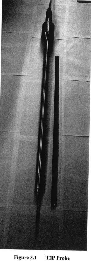
3.1 T2P Piezoprobe ₈₅

3.1.1 Physical Configuration 85

3.1.2 Pore Pressure Measurement 87

3.1.3 Temperature Measurement 88

3.1.4 Electrical Connections 88

3.2 Depth Locator Box 89

3.3 Atmospheric Pressure Transducer 90

3.4 Response Chamber 90

3.5 Porous Element Saturation System 90

3.6 Data Acquisition 91

3.7 Power Supply ₉₂

3.7.1 Power for Data Acquisition System and Laptop Computer 92

3.7.2 Power for T2P and Support Equipment 92

4 Field Test Procedures ₁₁₅

4.1 Assembly of T2P 115

4.2 Borehole Advancement 115

4.3 _{Penetration, Dissipation, and Extraction Procedures 116}

4.4 Sampling ₁₁₈

4.5 Data Collection Routines 118

4.5.1 Initial Response Configuration 118

4.5.2 Prepenetration Configuration 118

4.5.3 Penetration Configuration 119

4.5.5 Extraction Configuration 4.5.6 After Penetration Configuration 4.5.7 Final Response Configuration

4.6 Equipment Calibration

4.7 Resolution, Noise, and Stability of Transducers 4.8 Pressure Response Evaluation

4.9 Equipment Problems During the Field Test

5 Field Data

5.1 Penetration Records

5.1.1 Penetration Rate

5.1.2 Temperature Measurements

5.1.3 Pore Pressure Measurements

5.1.3.1 Individual Penetrations 5.1.3.2 Piecewise Penetration 5.2 Dissipation Records

5.2.1 Influence of Electrical Noise on Dissipation Data

5.2.2 Detachment Effects on Dissipation

5.3 Extraction Records 6 Interpretation of Field Data

6.1 Comparison of Dissipation Data 6.2 Time for 50% Dissipation (t50)

6.3 Brake Points

6.4 Determination of In-Situ Pore Pressure (u₀) 6.4.1 Full Dissipation

6.4.2 Inverse Time (1/t) Extrapolation 6.4.3 Two-Point Intersection Method

6.4.4 Comparison of Methods for Estimating In-Situ Pore Pressure

6.5 Determination of Hydraulic Conductivity (k)

7 Summary, Conclusions, and Recent Advancements 7.1 Summary of Research

7.1.1 Field Test Data 7.1.2 Data Interpretation

7.1.3 Recent T2P Modifications

7.1.3.1 Overview of Modifications

7.1.3.2 New Electrical Components and Power Source 7.1.3.3 Modified Housing Components

7.2 Conclusions References Appendix A Appendix B Appendix C 10 119 119 120 120 121 124 125 171 171 171 172 173 173 175 176 178 179 179 289 289 290 291 291 292 293 296 298 299 341 341 342 343 345 345 346 347 349 357 359 365 387

LIST OF TABLES

Table 2.1 Newbury Test Site Soil Properties (Paikowsky and Hart, 1998) 47

Table 2.2 Geologic Profile of Saugus Site (Varney, 1998) 49

Table 2.3 Numerical Values of the Model Parameters for Normally 51

Consolidated BBC, with K. = 0.537 (Levadoux, 1980)

Table 3.1 Relationship Between Thermistor Resistance and Temperature 95 (provided by General Electric, Inc.)

Table 4.1 Summary of Installation Details 127

Table 4.2 Field Test Channel Configurations 128

Table 4.3 Calibration Factors and Goodness of Fit (R2_{) 128}

Table 4.4 Resolution, Noise, and Drift of Transducers 129

Table 4.5 Pressure Change Between Initial and Final Zero Pressure Values 130

Table 5.1 Initial Zero Pressure Voltages 181

Table 5.2 Time from the Beginning of Dissipation to the Moment the Cross 181 Head Was Removed from the Drill String.

Table 6.1 Time to 50% Dissipation (t5 0) for the T2P 301

Table 6.2 Piezoprobe and Piezocone tso Values from the Saugus Site 301 (Varney, 1998)

Table 6.3 Dissipation Measurement Durations 302

Table 6.4 Ratio of Final Measured Pore Pressure (udiss) to Assumed In-Situ 302 Value (uo)

Table 6.5 Inverse Time Extrapolation Method for Determination of u) 303

-Tip Data

Table 6.6 Inverse Time Extrapolation Method for Determination of u. 304 - Shaft Data

Table 6.8 Comparison Between Inverse Time Extrapolation and Two-Point Matching Methods for T2P Data

Table 6.9 Values of Hydraulic Conductivity (k) from the T5 0 Matching

Method - T2P Tip Data

Table 6.10 Values of Hydraulic Conductivity (k) from the T50 Matching Method - T2P Shaft Data

12

305

306

LIST OF FIGURES

Figure 1.1 Geometry of the FMMG Piezoprobe (Ostermeier et al., 2001) and the DVTP-P (Schroeder, 2002)

Figure 1.2 Example of Inverse Time Extrapolation Method to Estimate In-Situ Pore Pressure

Figure 1.3 Calculation of Hydraulic Conductivity from Measured and Predicted Dissipation Behavior Using T50 Matching

(Whittle et at., 2001)

Figure 1.4 Modeled Dissipation Behavior of Dual-Pressure Probe as predicted with a Total Stress Soil Model

Figure 2.1 T2P Field Test Site Location (Paikowsky and Hart, 1998) Figure 2.2 Newbury Field Test Site Plan with Boring Locations

(based on figure from Degroot et al., 2004)

Figure 2.3 Newbury Test Site Soil Profile (Paikowsky and Hart, 1998) Figure 2.4 Water Table Elevation Measurements from the Newbury

Test Site (Paikowsky and Hart, 1998) Figure 2.5 Plasticity Chart

Figure 2.6 Stress History Profile for Newbury Site (Paikowsky and Hart, 1998)

Figure 2.7 Calculated and Measured Undrained Shear Strength at the Newbury Test Site (Paikowsky and Hart, 1998)

Figure 2.8 Cone Penetrometer Data from Three Penetrations (DeGroot, 2005) Figure 2.9 Saugus Site Plan (Varney, 1998)

Figure 2.10

Figure 2.11

Figure 2.12

Comparison of Piezoprobe Piecewise Penetration Records with Continuous Piezocone Penetration Records at Saugus

(Varney, 1998)

Index Properties and Stress History of BBC at the Saugus Site (Varney, 1998)

Field Vane Strength of BBC at the Saugus Site (Varney, 1998)

29 31 33 35 53 55 57 59 61 63 65 67 69 71 73 75

Figure 2.13 Figure 2.14 Figure 2.15 Figure 2.16 Figure 3.1 Figure 3.2 Figure 3.3 Figure 3.4 Figure 3.5 Figure 3.6 Figure 3.7 Figure 3.8 Figure 3.9 Figure 3.10 Figure 3.11 Figure 3.12 Figure 4.1 Figure 4.2 Figure 4.3

Laboratory Measurements of Soil Permeability at Saugus (Varney, 1998)

Newbury Test Site Soil Profile (Paikowsky and Hart, 1998) with Locations of T2P Tip Dissipation Measurements Schematic of the Method used to Calculate Strain, Stress, and Pore Pressure During Probe Penetration and Dissipation (Varney, 1998; Whittle et al., 1997)

Modeled Results for T2P Dissipation (courtesy of Hui Long, personal communication)

T2P Probe

Tip with Attached Thermistor Tube Needle

Transducer Block

Drive Tube with Drive Tube Nut Attached AW Coupling

Spin Collar

T2P Pore Pressure Measurement Locations Depth Locator Box (Varney, 1998)

Response Chamber (Varney, 1998)

Schematic of System used to Evacuate the Chamber in Preparation for Saturation of Filters (Varney, 1998) Schematic of the Deaired Water System used to Saturate Porous Elements (Varney, 1998)

Calibration of Original Tip Pore Pressure Transducer Calibration of Shaft Pore Pressure Transducer

Calibration of Replacement Tip Pore Pressure Transducer 14 77 79 81 83 97 99 99 101 101 103 103 105 107 109 111 113 131 133 135

Figure 4.4 Figure 4.5 Figure 4.6 Figure 4.7 Figure 4.8 Figure 4.9 Figure 4.10 Figure 4.11 Figure 4.12 Figure 4.13 Figure Figure Figure Figure Figure Figure Figure Figure Figure Figure 4.14 4.15 4.16 4.17 4.18 4.19 4.20 4.21 5.1 5.2

Calibration of Witness pore Pressure transducer Calibration of Temperature Probe in Ice Bath

Laboratory Stability Test of Atmospheric Pressure Transducer Calibration of Depth Box

Laboratory Stability Test of Original Tip Pore Pressure Transducer

Laboratory Stability Test of Shaft Pore Pressure Transducer Laboratory Stability Test of Replacement Tip Pore Pressure Transducer

Change in Initial Zero Pressure Values for the Pore Pressure Transducers

Drift of Initial and Final Zero Pressure Values Measured at the Tip

Drift of Initial and Final Zero Pressure Values Measured at the Shaft

Initial and Final Response Initial and Final Response Initial and Final Response Initial and Final Response Initial and Final Response Initial and Final Response Initial and Final Response Initial and Final Response

Checks for TP1_P1 Checks for TP 1_P2 Checks for TP1_P3 Checks for TP 1_P4 Checks for TP1_P5 Checks for TP 1_P6 Checks for TP2_P1 Checks for TP2_P2

TP1_P1 Change in Depth vs. Time during Penetration TP1_P2 Change in Depth vs. Time during Penetration

137 139 141 143 145 147 149 151 153 153 155 157 159 161 163 165 167 169 183 185

Figure 5.3 Figure 5.4 Figure 5.5 Figure 5.6 Figure 5.7 Figure 5.8 Figure 5.9a Figure 5.9b Figure 5.9c Figure 5.1 Oa Figure 5.1Ob Figure 5.1 Oc Figure 5.11a Figure 5.11b Figure 5.11 c Figure 5.12a Figure 5.12b Figure 5.12c Figure 5.13a Figure 5.13b Figure 5.13c Figure 5.14a TP1_P3 TP1_P4 TP1_P5 TP1_P6 TP2_P1 TP2_P2 TP1_P1 TP1_P1 TP1_P1 TP1_P1 TP1_P1 TP1_P1 TP1_P2 TP1_P2 TP1_P2 TP1_P3 TP1_P3 TP1 P3

Change in Depth vs. Time during Penetration Change in Depth vs. Time during Penetration Change in Depth vs. Time during Penetration Change in Depth vs. Time during Penetration Change in Depth vs. Time during Penetration Change in Depth vs. Time during Penetration Temperature vs. Time during Penetration Depth vs. Time during Penetration

Temperature vs. Depth during Penetration Change in Depth vs. Time during Penetration Penetration Pore Pressure vs. Time

Pressure vs. Depth during Penetration

Change in Depth vs. Time during Penetration Penetration Pore Pressure vs. Time

Pressure vs. Depth During Penetration

Change in Depth vs. Time During Penetration Penetration Pore Pressure vs. Time

Pressure vs. Depth During Penetration

TP1_P4 Change in Depth vs. Time During Penetration TP1_P4 Penetration Pore Pressure vs. Time

TP1_P4 Pressure vs. Depth During Penetration

TP1_P5 Change in Depth vs. Time During Penetration

16 187 189 191 193 195 197 199 199 201 203 203 205 207 207 209 211 211 213 215 215 217 219

Figure 5.14b Figure 5.14c Figure 5.15a Figure 5.15b Figure 5.15c Figure 5.16a Figure 5.16b Figure 5.16c Figure 5.17a Figure 5.17b Figure 5.17c Figure 5.18 Figure 5.19 Figure 5.20 Figure 5.21 Figure 5.22 Figure 5.23 Figure 5.24 Figure 5.25 TP1_P5 TP1_P5 TP1_P6 TP1_P6 TP1_P6 TP2_P1 TP2_P1 TP2_P1 TP2_P2 TP2_P2 TP2_P2

Penetration Pore Pressure vs. Time Pressure vs. Depth During Penetration

Change in Depth vs. Time During Penetration Penetration Pore Pressure vs. Time

Pressure vs. Depth During Penetration

Change in Depth vs. Time During Penetration Penetration Pore Pressure vs. Time

Pressure vs. Depth During Penetration

Change in Depth vs. Time During Penetration Penetration Pore Pressure vs. Time

Pressure vs. Depth During Penetration

Ratio of Tip Pore Pressure over Shaft Pore Pressure vs. Depth During TPI_P3

Ratio of Tip Pore Pressure over Shaft Pore Pressure vs. Depth During TP1_P4

Ratio of Tip Pore Pressure over Shaft Pore Pressure vs. Depth During TP1_P5

Ratio of Tip Pore Pressure over Shaft Pore Pressure vs. Depth During TP1_P6

Ratio of Tip Pore Pressure over Shaft Pore Pressure vs. Depth During TP2_P1

Ratio of Tip Pore Pressure over Shaft Pore Pressure vs. Depth During TP2_P2

Combined Penetration Plots from TP1_P3, TP1_P4, TP1_P5, TP1 P6, and TP2_P2 TP 1_P3 Dissipation Data 219 221 223 223 225 227 227 229 231 231 233 235 235 237 237 239 239 241 243

Figure 5.26 Figure 5.27 Figure 5.28 Figure 5.29 Figure 5.30 Figure 5.31 Figure 5.32 Figure 5.33 Figure 5.34 Figure 5.35 Figure 5.36 Figure 5.37 Figure 5.37c Figure 5.38 Figure 5.39 Figure 5.39c Figure 5.40 Figure 5.40c Figure 5.41 Figure 5.41c Figure 5.42 Figure 5.42c TP1_P4 Dissipation Data TP1_P5 Dissipation Data TP 1_P6 Dissipation Data TP2_P1 Dissipation Data TP2_P2 Dissipation Data

TP1_P3 Installation Effects on Pore Pressure Record TP1_P4 Installation Effects on Pore Pressure Record TP1 _P5 Installation Effects on Pore Pressure Record TP1_P6 TP2_P1 TP2_P2 TP1_P3 TP1_P3 TP1_P4 TP1_P5 TP1_P5 TP1_P6 TP1_P6 TP2_P1 TP2 P1

Installation Effects on Pore Pressure Record Installation Effects on Pore Pressure Record Installation Effects on Pore Pressure Record Extraction Data

Extraction Data - Pressure vs. Depth

Extraction Data - Pressure vs. Time during Extraction Extraction Data

Extraction Data - Pressure vs. Depth Extraction Data

Extraction Data - Pressure vs. Depth Extraction Data

Extraction Data - Pressure vs. Depth TP2_P2 Extraction

TP2_P2 Extraction Data

Data - Pressure vs. Depth

18 245 247 249 251 253 255 257 259 261 263 265 267 269 271 273 275 277 279 281 283 285 287

Figure 6.1 Combined Normalized Dissipated Pore Pressure Records from Tip 307 Measurements

Figure 6.2 Combined Normalized Dissipated Pore Pressure Records from Shaft 309 Measurements

Figure 6.3 Values of t5 0 from T2P Dissipation Data 311

Figure 6.4 Tip and Shaft Dissipation Records for TP1_P1 313

Figure 6.5 Tip and Shaft Dissipation Records for TP 1_P5 315

Figure 6.6 Tip and Shaft Dissipation Records for TP2_P2 317

Figure 6.7 1/t Method on TP2_P2 Dissipation Record with t=100sec 319 Figure 6.8 1/t Method on TP2_P2 Dissipation Record with t=166.7sec 319 Figure 6.9 1/t Method on TP2_P2 Dissipation Record with t=250sec 321 Figure 6.10 1/t Method on TP2_P2 Dissipation Record with t=500sec 321 Figure 6.11 1/t Method on TP2_P2 Dissipation Record with t=1000sec 323 Figure 6.12 Results from the 1/t Method for T2P Tip and Shaft 325

Dissipation Data - Natural Scale

Figure 6.13 Results from the 1/t Method for T2P Tip and Shaft 327

Dissipation Data - Logarithmic Scale

Figure 6.14 Convergence of the Pore Pressure Predicted by the Inverse 329 Time Extrapolation Method to the Dissipated Pore Pressure

Value for the Piezoprobes (Varney, 1998)

Figure 6.15 Convergence of the Pore Pressure Predicted by the Inverse 331 Time Extrapolation Method to the Dissipated Pore Pressure

Value for the Piezocones (Varney, 1998)

Figure 6.16 Two-Point Matching Method - TP1_P3 Dissipation Data 333 Figure 6.17 Two-Point Matching Method - TP1_P4 Dissipation Data 335 Figure 6.18 Two-Point Matching Method - TP1_P6 Dissipation Data 337

Figure 6.19 Hydraulic Conductivity as Determined from the T5o Matching Method on T2P Dissipation Data

Figure 7.1 Modified Connection Between Drive Tube and New Data Acquisition System

Figure 7.2 T2P Shroud

Figure 7.3 Operation of Shroud

20

339

351

353 355

1 INTRODUCTION

The in-situ temperature and pore water pressure of sub-seafloor sediments are of great interest to both the scientific community and the offshore oil and natural gas industries. Fluid pressure and temperature affect the solubility of gas in water and impact the permeability of marine sediments (Kvenvolden, 1993). The migration of pore fluids and dissolved gases is driven by the permeability of these sediments and in-situ pressure and temperature gradients. Excess pore pressures within continental slopes have been linked to marine slope failures (Dugan and Flemings, 2002). Direct measurements of in-situ pore pressures within sub-seafloor sediments have been limited by the time and cost required to collect this data. The Integrated Ocean Drilling Program (IODP), an international research program involved in the exploration of marine hydrogeology, has obtained high-quality direct sub-seafloor temperature and pressure measurements through the use of long-term, seafloor observatories installed in boreholes (i.e., Circulation Obviation Retrofit Kits or CORKS). However, the time and expense associated with the installation and maintenance of these observatories make this approach unrealistic for routine data collection.

IODP and the oil and gas industries have also used penetration devices to measure the in-situ pore pressure and permeability of marine sediments. The first modern penetration device was the electric cone (de Ruiter, 1970), which has both an axial load cell to measure tip resistance and a friction sleeve to calculate soil/steel interface resistance. Continuous measurements of tip and friction resistance collected during cone penetration are correlated with variations in soil properties, thus providing an efficient method to determine subsurface profiles. However, it was not until Senneset (1974) developed the piezocone by adding a pressure transducer to the electric cone, that a single tool could concurrently measure pore pressure, tip resistance, and frictional resistance in the same borehole (Varney, 1998). The combination of pore pressure and tip force measurements in a single device improved the accuracy of the modern penetrometer as a profiling tool.

Penetration devices, such as the piezocone, are also commonly used to measure pore pressure during penetration of sediments at the base of boreholes drilled into the

seafloor. The insertion of the tool creates a pressure pulse, the rate of which is controlled by the radius of the penetrometer and the permeability and compressibility of the surrounding sediments.

Traditionally, piezocones have been deployed in this manner by industry and the Davis-Villinger Temperature-Pressure Probe (DVTP-P) has been used by the IODP. However, the time required to reach full dissipation using either of these tools can exceed 24 hours (Whittle et al., 2001), which is a prohibitively long time for a drilling vessel to remain stationary on the ocean surface while pressure measurements are being recorded. In order to address this problem, Fugro-McClelland Marine Geosciences, Inc. (FMMG) developed the FMMG piezoprobe, which measures pore pressure near the tip of a 26.5 cm long, 0.64 cm wide, tapered extension piece that is attached to the end of a standard piezocone shaft. This design is intended to accelerate the dissipation of penetration-induced excess pore pressure, thus reducing the required time to reach the in-situ value.

The geometries of the piezoprobe and the DVTP-P devices differ dramatically, as shown in Figure 1.1. Each tool measures pressure through a porous element near its tip. However, the piezoprobe measures pressure at a point located 2.4 cm above its tip, while the DVTP-P's porous element is located 10 cm above its tip. It has been found that the geometry of the DVTP-P causes dissipation to occur more slowly than it does for the piezoprobe in soils with similar permeability and compressibility. In addition, the piezoprobe is significantly narrower then the DVTP-P; therefore, the magnitude of the pressure pulse induced by the DVTP-P is considerably greater than that caused by the piezoprobe. It is also suspected that DVTP-P penetration may cause formation failure, due to the relatively large size of this tool. Since a drilling vessel must remain stationary during the deployment of a penetration device, it is impractical for a tool to remain at the measurement location for longer than a few hours. The time required for full dissipation of excess pore pressure induced by either DVTP-P or piezoprobe penetration is considerably longer than this; therefore, these tools are impractical for routine measurements. Therefore, an important goal of the IODP has been to develop a device that can measure in-situ pressures in shorter time periods.

In an effort to infer in-situ pore pressures from incomplete dissipation records, the inverse time extrapolation method has traditionally been used. For this method, pressure is plotted versus inverse time on a natural scale. A tangent line is then extended from the final portion of the incomplete dissipation record, with the y-intercept assumed to be the in-situ pressure. Figure 1.2 illustrates how this construction is used on a partial dissipation record, in which the in-situ pore pressure is estimated at 166.7 and 500 seconds after the start of dissipation. As indicated in this figure, the accuracy of the estimate of in-situ pore pressure improves as the length of the dissipation increases. Because the dissipation data is non-linear at large time scales, this method typically overestimates in-situ pressures for both the piezoprobe and the DVTP-P (Whittle et al., 2001).

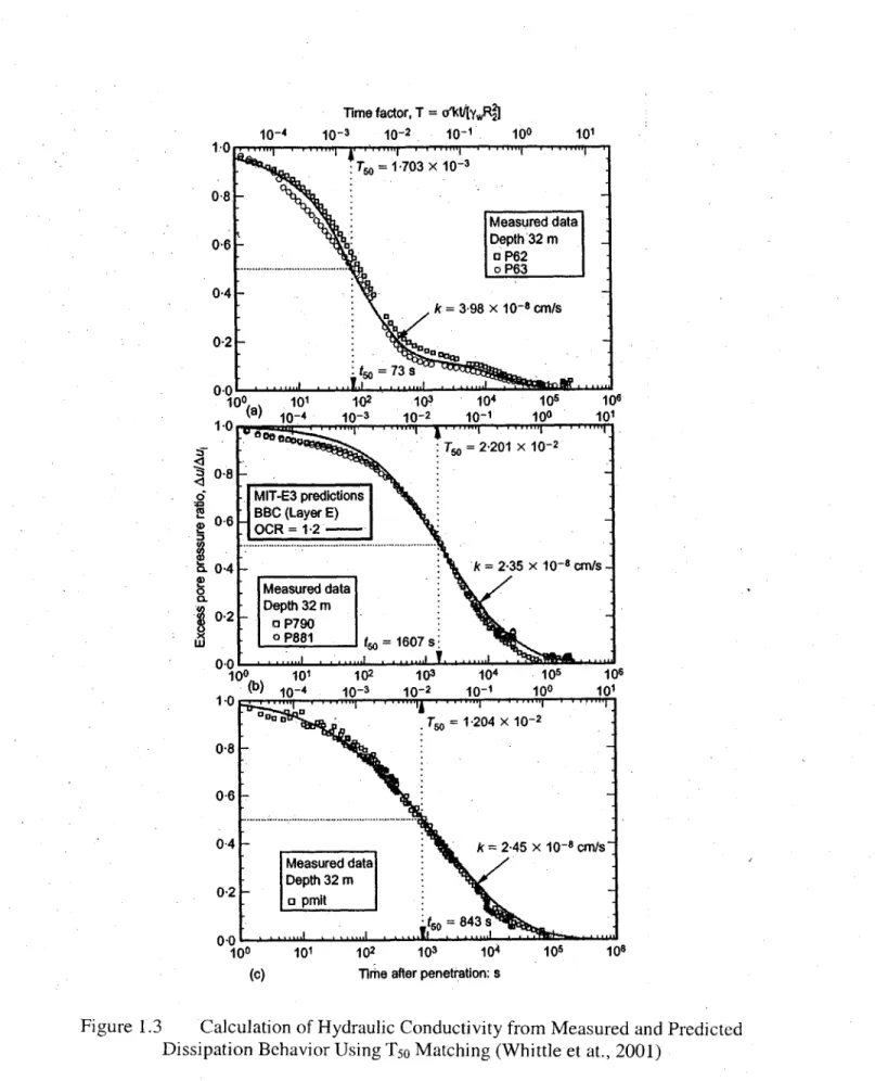
In order to improve the reliability of estimates of hydraulic conductivity from incomplete dissipation records, the MIT geotechnical group (Aubeny et al., 2000; Whittle, 1992; Whittle and Sutabutr, 1999, Whittle, 2001) used the Strain Path Method (SPM [Baligh, 1985]) in combination with effective stress soil models based on elasto-plasticity (MIT-E3 [Whittle et al, 1994]) to predict changes in stress during post-penetration consolidation. In this manner, a characteristic dissipation curve was derived for the penetrometer, based on specific input soil parameters. The dissipation of penetration-induced pore pressure is plotted versus a dimensionless time factor, from which hydraulic conductivity can be derived,

T =r k

yR Equation 1.1

where T is the model time factor, k is hydraulic conductivity, y, is the unit weight of water, R2 is the radius of the larger-diameter shaft of the piezoprobe, -' is the in-situ mean effective stress at the pore pressure measurement point, and t is the measured time. The T50 matching method can be used to calculate hydraulic conductivity from the

measured and predicted curves by matching the model predicted time factor for 50% dissipation (T50) with the measured time (t50) required for 50% dissipation of excess pore pressures. Hydraulic conductivity can then be calculated in the following manner:

k = 5 Equation 1.2 7 1 t50

Figure 1.3 shows how this technique was used to estimate hydraulic conductivity from measured and predicted dissipation of excess pore pressure for the FMMG piezoprobe.

The MIT geotechnical group also introduced a novel method for predicting in-situ pore pressures from incomplete dissipation records using SPM in combination with either effective stress or total stress soil models. This technique, referred to as the two point matching method, was used to improve the piezoprobe design. Whittle et al. (1997; 2001) predicted that concurrent measurements of pore pressure at two locations on the surface of a tapered probe could be used to make reliable predictions of in-situ pressures and to provide a consistent approach for controlling the required dissipation measurement duration. Figure 1.4 illustrates the predicted dissipation behavior for a dual-pressure probe, in which pore pressures are measured at both the tip (radius = 0.6 cm) and shaft (radius = 3.6 cm). This figure shows that approximately 90% dissipation of excess pore pressure will occur at the tip of a tapered probe when the magnitudes of dissipated pore pressure (u-u) are identical at both the tip and shaft. Once this intersection point is reached, it is possible to predict the in-situ pore pressure from incomplete dissipation data. Therefore, this approach provides a practical method for controlling dissipation measurement duration (i.e., data must only be collected until the intersection point is reached). It has been estimated that the intersection point will occur in as little as 30 minutes after the onset of dissipation for a piezoprobe in sub-seafloor sediment at the Hydrate Ridge, located offshore from Oregon, USA (Flemings et al., 2003). It has also been found that the intersection point will occur at approximately 90% dissipation of excess pore pressure at the tip, regardless of soil properties or stress history. Hence, it is not necessary to measure the soil properties of the deposit of interest or to run additional numerical simulations before using this method. The MIT group has verified the validity of this technique by combining and analyzing piezocone and FMMG piezoprobe dissipation data that was collected at a site in Saugus, Massachusetts (Varney, 1998).

In summary, a piezoprobe that measures pore pressure at multiple locations will improve the estimation of in-situ pore pressures at deep-water sites in shorter times than was previously possible with existing penetration tools.

1.1 Purpose of this Project

This thesis describes the design and land-based field evaluation of a probe prototype (referred to as the T2P) that measures temperature at its tip and pore pressure at two monitoring points with different radii. The T2P field data are presented, interpreted, and compared with the results of a previous land-based field evaluation of several piezoprobes and piezocones that was performed by Varney (1998).

This thesis is part of a larger project funded by the National Science Foundation. The overall goal of this project is to produce a dual-pressure probe capable of offshore deployment by the IODP. Since the 2004 T2P field test, various modifications have been made to the T2P in preparation for an anticipated offshore deployment in June and July of 2005. These design changes are discussed in Chapter 7 and illustrated in Appendix C.

1.2 Organization of Thesis

Chapter 2 presents the results of several geotechnical investigations previously performed at the Newbury field test site in Massachusetts. A summary of the theoretical framework used to create the model predictions presented in this thesis is also included in this chapter.

Chapter 3 describes the geometry of the tool, design considerations, and the equipment used during the December 2004 T2P field test. The equipment discussed in this chapter includes the prototype T2P housing, transducers, electrical connections, data acquisition, and support equipment.

Chapter 4 discusses the manner in which the field test was conducted and the steps taken to ensure the collection of high-quality data. The field stability and resolution of the pore pressure measurements are also examined in this section.

Chapter 5 presents the T2P temperature and pressure data collected during the field test. The resulting penetration, dissipation, and extraction records are examined for the influence of electrical noise and other equipment problems. The T2P dissipation data

is compared with the piezoprobe and piezocone dissipation records, collected by Varney (1998).

Chapter 6 discusses the various methods used to interpret the T2P dissipation data. The values of in-situ pore pressure and permeability inferred from the T2P

dissipation records are also presented in this chapter.

Chapter 7 summarizes the results and conclusions from the T2P field test and describes the advancements in the T2P design that have been implemented to date.

590mm'

10~rM4

23.6mm-

OmMs-DVTP-P

LU

K+fl4

-55.5mm

Piezoprobe

pressure

transducer

.

Jmm

35.6mm

4-6.4mm

pressure transducer

Geometry of the FMMG Piezoprobe (Ostermeier et al., 2001) and the DVTP-P (Schroeder, 2002) -

1,1nmM

4-11.7mm

thermistor

U= estimated in situ pore pressure I I 777777t I I 0.01 0.008 0.006 1/T (1/seconds) 0.004 0.002

Example of Inverse Time Extrapolation Method to Estimate In-Situ Pore Pressure

500 450 400 350 300 '0 250 ~'200 U 0.012 150 100 50 0 0 Figure 1.2

Time factor, T = o'kt[ywRll 10-4 10-3 10-2 10-1 1-.0 0.8. 0-6 0-4 0-2 00 1.0 100 101 102 103 104 106 106 10-3 10-2 10-1 100 101 T= 2-201 X 10-2 MIT-E3 predictions BB3C (Layer E) OCR = 1.2-2 k = 2-35 x 10-8 CM/s Measured data Depth 32 m 7 P790 I 0 P881 _{to 1607 s} 100 101 (b) _10-4 1.0J 0.8 0-6 0-4 0-2 n0 100 (c) 102 103 104 106 106 10-3 10-2 10-1 100 101 101 102 103 104 105 106

Tirme after penetration: s

Figure 1.3 Calculation of Hydraulic Conductivity from Measured and Predicted Dissipation Behavior Using T50Matching (Whittle et at., 2001)

T= 1-703 x 10-3 Measured data Depth 32 m o P62 ...--..-..--.-..--.-...-... _{o P63} k =398 x 10-8 cm/s Daa73 t = 73 s 0 101 (a) 1O-4 0-8 6 0-6 a0.4_0-4 0. 0-2 x w

4

bo

10

10

10

T=ct/R;

Modeled Dissipation Behavior of Dual-Pressure Probe as predicted with a Total Stress Soil Model

R:2 -R Shaf R -L

S14

10

08

460.6

0.4

V0.2

w

10

2 BACKGROUND

This chapter provides background information concerning the Newbury site used to perform the 2004 T2P field, a description of the scope of the field program, and a brief overview of the theoretical framework used to interpret the dissipation data. This chapter also includes background information for a site in Saugus, Massachusetts at which Varney (1998) evaluated the performance of several piezocones and piezoprobes. Penetration data collected at the Saugus site will be compared with T2P data in Chapters

5 and 6.

2.1 T2P Field Test Site

The field test site is located in Newbury, Massachusetts, next to the Newburyport Massachusetts Bay Transportation Authority (MBTA) train station. Refer to Figure 2.1 for the site location. The first subsurface studies at the site were conducted in the 1930's, for the construction of a foundation for a multi-span, concrete-reinforced bridge along Route 1 in Newbury (Paikowsky and Hart, 1998). This bridge, completed in 1935, was demolished in 1996. Additional geotechnical studies were performed at the site in the 1988 and throughout the 1990's for the construction of a replacement bridge. A total of 36 borings were completed at the site before the 2004 T2P field test (Paikowsky and Hart, 1998).

This site was chosen as the initial test location for the T2P because it contains a 9 to 12 meter-thick deposit of BBC, close to the ground surface. A detailed plan of the site is shown in Figure 2.2. The plan includes borings from previous research projects and the three borings created and used for the 2004 T2P field test (Borings TP1, TP2, and LI). The average ground elevation at the site is approximately 5.4 meters above mean sea level (DeGroot et al., 2004). The test site is bordered to the north by the MBTA station exit ramp, to the south by the foundation of the overlying Route 1 bridge, to the east by a utility road, and to the west by the MBTA commuter train tracks. Several piers supporting the bridge are located in the site area. The presence of the bridge over the site limits the available overhead clearance for drilling operations to approximately 8 meters.

2.1.1 Summary of Newbury Site Subsurface Conditions

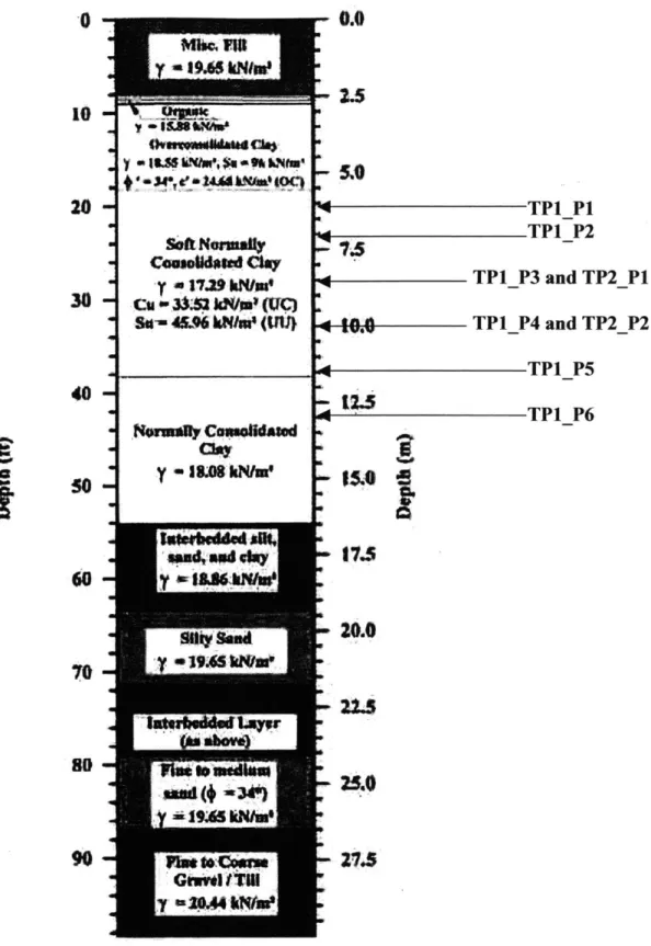
The following description of the Newbury test site deposit was abstracted from Paikowsky and Hart (1998), and is based upon field and laboratory testing of soil samples, performed at the University of Massachusetts at Lowell. Figure 2.3 illustrates an average geological cross-section of the site. From the ground surface downward, the general soil profile consists of 2.4 meters of granular fill, consisting of very dense, brown sand and gravel, intermixed with concrete fragments, overlying approximately 0.3 meters of organic silt and peat. Below the organic layer is a 13.7-meter thick deposit of Boston Blue Clay (BBC), a marine clay deposited by glacial meltwater. The BBC is composed of approximately 2.7 meters of medium stiff to very stiff, overconsolidated clay, over 6.1 meters of very soft to soft, plastic, normally to slightly overconsolidated clay, and 4.9 meters of soft, plastic, normally consolidated clay. A 2.9-meter thick layer of interbedded silt, fine sand, and silty clay lies beneath the BBC. Below this interbedded deposit is a 2.4-meter thick stratum of silty sand. A second interbedded deposit of silt, fine sand, and silty clay, approximately 2.3 meters thick, underlies the silty sand. Beneath this interbedded deposit is 2.4 meters of medium dense to dense, fine to medium sand. Below the fine to medium sand is a dense glacial till, composed of medium dense to dense, fine to coarse sand and gravel, with traces of rock fragments and silt. Underlying the till is mylonitic, basalt bedrock.

Figure 2.4 plots water table elevation measurements made at the Newbury test site by Paikowsky and Hart (1998) between March 5 and September 4, 1996. Over this period, the depth of the water table generally ranged from 1.75 and 2.5 meters.

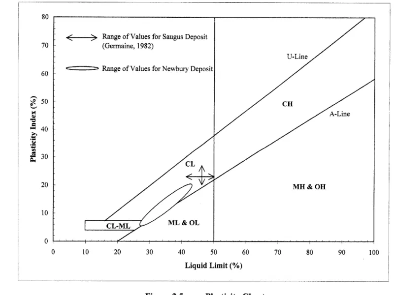
The index and engineering properties for the Newbury BBC deposit are listed in Table 2.1 and Figure 2.5 is a plasticity chart indicating the location of the Newbury site BBC. In the United Soil Classification System (USCS), the Newbury site BBC plots above the A-line and is designated CL, i.e., low-plasticity clay.

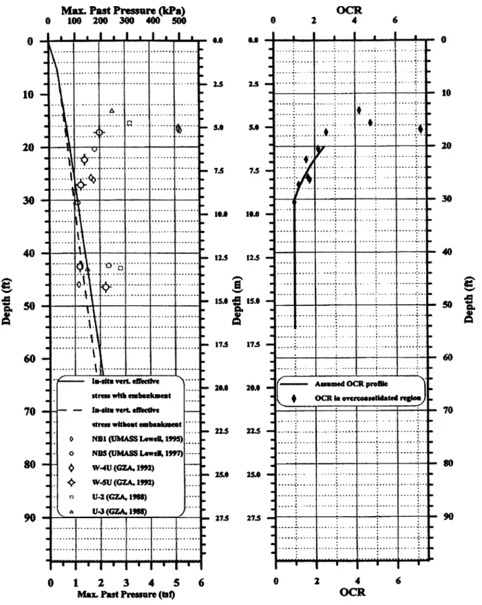
The stress history profile of the BBC is shown in Figure 2.6. The preconsolidation pressure is at a maximum at the top of the clay, decreases to a minimum at an approximate depth of 9 meters, and then increases linearly with depth. Figure 2.5

indicates that the overconsolidation ratio (OCR) of the deposit ranges from 4 to 7 at the top, decreases to 1 within the upper 7 meters, and then remains constant with depth.

Figure 2.7 presents the undrained strength profile of the clay, as measured with SHANSEP, DSS, UU, and UC laboratory tests. This figure indicates that the undrained shear strength approaches 100 kPa near the top of the deposit, and then ranges from 15 to 50 kPa below a depth of 5.5 meters. The trend in strength is similar to that of the preconsolidation pressure profile. It should be noted that the engineering properties for the Newbury BBC deposit have not been independently verified at MIT.

Data from several piezocone profiles perfomed at the Newbury site by Jacubowski (2004) are shown in Figure 2.8.

2.2 Saugus Field Test Site

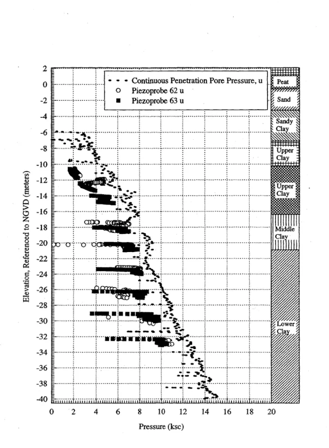
Since the mid-1960's, MIT has conducted various field programs at a well-documented site in Saugus, Massachusetts, including a 1996 field evaluation of two FMMG piezoprobes, two standard piezocones, and one MIT piezocone (Varney, 1998). A detailed plan of this site, located approximately 10 miles from MIT, is shown in Figure 2.9. The plan shows the locations of boreholes used for both the 1996 field program and for previous research projects. For the 1996 field test, two borings (790PUSH and 881PUSH) were used to perform continuous piezocone penetration soundings, and five borings were installed to collect long-term dissipation data: one for each piezoprobes (PP62 and PP63), one for each piezocone (PC790 and PC881), and one for the MIT piezocone (MIT). Three borings (M206A, M206B, and M206C) were used to install piezometers and one borehole (B96) was installed to collect undisturbed soil samples. The pore pressure data from a continuous piezocone profile and piezoprobe penetration records collected by Varney are plotted versus depth and are shown in Figure 2.10. For additional information on the manner by which the 1996 field program was conducted, refer to Varney (1998).

2.2.1 Subsurface Conditions at the Saugus Site

The following description of subsurface conditions at the Saugus field test site was summarized from Varney (1998) and is based on data collected during the 1996 field

test and from previous research programs. The soil profile is listed in Table 2.2. From the surface downward, this profile consists of 1.2 to 1.8 meters of peat overlying 5 meters of sand. Below the sand is a 37-meter thick deposit of BBC, over glacial till. The upper 4 meters of the BBC (Zone A) are stiff and strongly interbedded with sand. The next 3 meters of the clay (Upper Clay Zone B) are also stiff, with numerous sand layers. Upper Clay Zone B is significantly desiccated, with large variations in piezocone penetration resistance. The next 6 meters (Upper Clay Zone C) are stiff and have thicker clay layers, with large disparities in penetration resistance. Below Upper Clay Zone C is a transition zone (Middle Clay Zone D), which exhibits a constant to decreasing penetration resistance with depth and is considerably more uniform than the clay above. The remaining 24 meters of BBC (Lower Clay Zone E) are softer and more uniform, with little sand.

The index properties and stress history for the Saugus site clay deposit are shown in Figure 2.11. The natural water content of the clay gradually increases from roughly 30% near the top to approximately 45% in the soft clay, then is constant throughout the rest of the deposit (Germaine, 1980). The plasticity index ranges from 15 to 30% and is generally lower and more variable in the upper 15 meters. The location of the Newbury site BBC. Like the Newbury BBC, the clay at the Saugus site is designated as CL (low-plasticity clay) in the USCS, and plots above the A-line in a plasticity chart, as shown in Figure 2.5.

Figure 2.11 indicates that the OCR of the clay is at a maximum of approximately 6 near the top of the deposit, and then decreases with depth. The scatter of calculated OCR values is larger in the upper layers. The BBC is normally consolidated below a depth of roughly 24 meters.

The undrained strength profile, as determined with a Geonor field vane, is presented in Figure 2.12. The undrained strength of the clay is larger and more scattered near the top of the deposit and then increases linearly with depth in Lower Clay Zone E.

Figure 2.13 presents laboratory measurements of the hydraulic conductivity of the clay. The values range from approximately 3xl06 cm/s at the top of the deposit, to 3x10-8 cm/s within the normally consolidated zone.

2.3 Comparison between the Newbury and Saugus Clay Deposits

Both the Newbury and Saugus BBC deposits are overconsolidated near the top and normally consolidated at depth. The water contents of the normally consolidated sections of both deposits have similar ranges and average values; however the Newbury BBC has a lower liquid limit and plasticity index than the Saugus clay. In addition, the undrained shear strength of the normally consolidated section of the Saugus deposit, as measured with a field vane, is generally higher than the undrained strength of the normally consolidated portion of the Newbury deposit, as measured with a field vane.

2.4 Scope of 2004 T2P Field Program

The T2P field program had a number of goals: 1) evaluate the performance of the tool in a controlled environment and compare the quality of the T2P penetration and dissipation data with previously collected piezoprobe and piezocone data; 2) assess the robustness of the individual mechanical and electrical probe components; 3) determine the ease of T2P field assembly and disassembly; 4) collect and assess several long-term T2P dissipation records that would not be possible to obtain during a sea deployment; 5) evaluate the resulting dissipation records in an attempt to optimize the final T2P tip geometries; 6) examine the effectiveness of the two-point matching method in calculating in-situ pore pressures from T2P dissipation data; 7) collect and evaluate temperature measurements during penetration and dissipation in order to assess the responsiveness and accuracy of the T2P temperature sensor; 8) determine the success of the T50 matching method in calculating in-situ permeabilities from T2P dissipation records.

The 2004 T2P field test ran from Tuesday, December 14th to Monday, December

20th . Two boreholes (TPl and TP2) were installed to collect penetration, dissipation, and extraction data. A third borehole, B104A, was installed to obtain samples of the BBC deposit; however, the collected samples have not yet been analyzed. The borehole locations were controlled by the geometry of the site and the presence of pre-existing boreholes.

A cargo van was brought to the site to house the data acquisition system, computers, power supply, and support equipment. The van also served as a shelter from

the elements for the personnel conducting the field test. As the site was not secure after dark, the van was locked with the field test equipment inside when the site was not manned. Power for the data acquisition system and accompanying computers was provided by the van's battery during the day and by an external battery at night. The van's engine was left running during the day to prevent the drainage of the vehicle's battery and to keep the field personnel warm. Power for the T2P's transducers was provided by an external battery at all times.

New Hampshire Boring, Inc. was subcontracted by Pennsylvania State University to install the boreholes, collect soil samples, and supply the drill rig and standard drilling and sampling equipment, the drilling operator, driller's apprentice, and drill rods.

2.4.1 Penetrations

Although dissipation measurements were a main focus of the field program, penetration data was also collected for several reasons. Recording temperature and pressure measurements during penetration at a fast sampling rate provides an opportunity to field-evaluate the response time of the temperature and pressure transducers. By examining the variation in excess pore pressure generated during each penetration, it is also possible to assess the intensity of layering within the soil deposit. Additionally, the penetration pore pressure records helped define the initial pressure (ui) that is used in the dissipation analysis. The magnitudes of penetration-induced pore pressure can also be used to make comparisons between different sites and devices and to determine if normalized values of penetration pore pressure (u/a'v) relate to the OCR of the deposit.

2.4.2 Dissipations

A major goal of the field program was to measure excess pore pressure dissipation data with the T2P. Both short (approximately one hour or less) and long (overnight) dissipation records were collected. By recording several overnight dissipations, it was hoped that full dissipation of excess pore pressures would occur, in order to compare the in-situ pore pressures measured after full dissipation with the values calculated from partial dissipation records. However, the available time for dissipation measurements was limited during the field test and, as discussed in Chapter 6, it is

uncertain if full dissipation occurred during any of the records. A total of eight dissipations were recorded during the field test, and all took place at depths between 6.1 and 12.8 meters below ground surface (bgs), within the BBC deposit. Six of the dissipations (TP1_P3, TPlP4, TP1_P5, TP1_P6, TP2_P1, andTP2_P2) occurred within the normally consolidated portion of the BBC. Figure 2.14 illustrates the locations within

the soil deposit at which the eight dissipations took place.

2.5 Theoretical Framework for Predictions

This section presents a brief description of the theoretical analyses used to model the dissipation of excess pore pressures induced by penetration of BBC. The intention is to provide sufficient information to allow duplication of the theoretical results. Much of the following was summarized from Varney (1998), where a more complete discussion of the analytical details can be found. Additional information was provided by Hui Long, a PhD candidate at Pennsylvania State University, who performed the theoretical analyses for the T2P.

The analyses used to predict the consolidation of clay around the T2P were performed in two main phases:

1) Simulation of undrained penetration of clay by the T2P, using the Strain Path Method (SPM [Baligh, 1985]).

2) Finite element calculations of pore pressure dissipation.

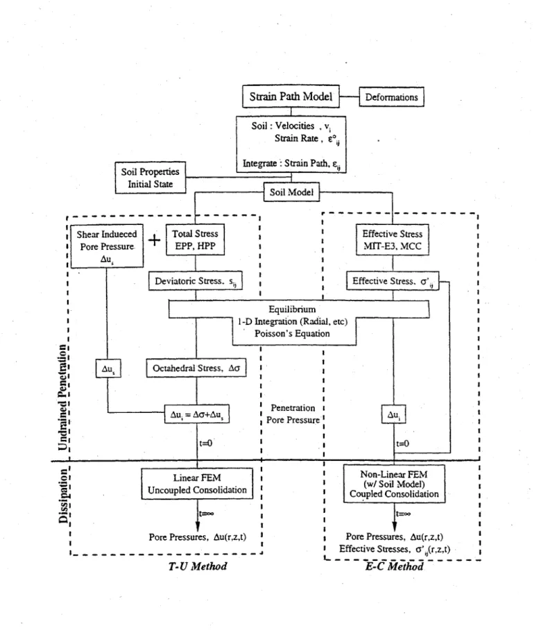
These two phases are shown schematically in Figure 2.15. SPM is an analytical framework that predicts the distortion caused by deep, quasi-static penetration of homogeneous clay by a penetrometer. SPM assumes that the soil deformations are effectively independent of the shear strength of the soil. SPM was used to determine the strains that occur when the T2P penetrates in an undrained shearing mode.

To model the geometry of the probe, the "method of sources and sinks" (Weinstein, 1948; Rouse, 1959) was used. Since the T2P is axisymmetrical, its outer surface could be modeled using a series of line sources and sinks distributed along the centerline of the body. Levadoux and Baligh (1980) originally used this technique for 180 and 60' cone penetrometers. The T2P geometry was modeled by Long using 300

uniformly distributed source-sink combinations, although there are an infinite number of source-sink distributions that can match the probe geometry.

Once the probe geometry is accurately modeled and the penetration displacements determined by SPM, either a total stress soil model with uncoupled consolidation (T-U analysis) or an effective stress soil model with coupled consolidation (E-C analysis) could then be used to predict the soil response. E-C analyses of dissipation behavior utilize the time factor presented in Chapter 1,

o-'kt

T = 2 Equation 1.1

y,2

which involves soil permeability (k), in-situ mean effective stress (o'), and the unit weight of water (y,). T-U analyses, which do not account for changes in effective stress that take place during consolidation, utilize a different time factor,

T = Ct Equation 2.1

R 2

where c is a coefficient of consolidation (L2_{/T) that controls the rate of pore pressure} dissipation, t is the elapsed time from the end of penetration, and R2 is the radius of the larger-diameter shaft of the piezoprobe. Both E-C and T-U analyses can provide realistic predictions of the dissipation behavior of penetrometers (Whittle et al., 2001). However, because T-U analyses do not involve hydraulic permeability, k cannot be determined using this method of analysis.

A T-U analysis was utilized for the analyses of the T2P field test results, i.e. a total stress soil model (MIT-TI [Levadoux, 1980]) was used to simulate the pore pressure build-up and the dissipation was modeled as uncoupled consolidation using the

ABAQUSTM

finite element code. Table 2.3 lists the input soil parameters that were used

in the analysis. Since no data were available for the Newbury site, model parameters for resedimented BBC were used in the model (for additional information regarding these parameters, refer to Levadoux, 1980). The finite element mesh used to model the T2P geometry consists of 3861 elements and 4000 nodes, and involves 4-node elements.

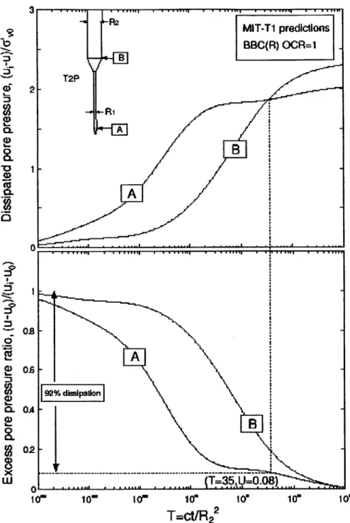
Figure 2.16 illustrates typical MIT-TI predictions of excess pore pressure dissipation in normally consolidated, resedimented BBC, as measured at the tip and shaft of the T2P. The top plot in this figure presents the results in terms of normalized dissipated excess pore pressures ((ui-u)/o o) and the bottom plot in terms of the excess pore pressure ratio ((u-u)/(ui-uo)). As mentioned in Chapter 1, an intersection point occurs when the magnitudes of dissipated pore pressure (ui-u) are identical at both the tip and shaft. For a particular soil type, stress level, and probe geometry, this intersection corresponds to a characteristic point on the normalized pore pressure ((u-u)/(ui-u0)) dissipation curve (Varney, 1998). Using the input soil parameters listed in Table 2.3, the theoretical results predict that the intersection point will occur at 92% dissipation of excess pore pressure at the T2P tip. Thus, by measuring ui and the tip pore pressure at the time of intersection (u), the in-situ pressure can be calculated by setting

(u-u2pt)/(ui-u2pt) = 0.088, where u2pt is the in-situ pore pressure calculated using the two-point intersection method. Hence, once the intersection point has been reached, in-situ pore pressures can be determined from incomplete dissipation records, thus reducing the required duration for dissipation measurements.

The bottom plot of Figure 2.16 shows that normalized pore pressures measured at the tip exhibit an inflection point or "brake point" at which the rate of change of normalized pore pressures significantly decreases. It is believed that this brake point occurs as the pressure pulse generated by the penetration of the larger diameter cone begins to affect pressure measurements made at the tip. Varney (1998) reported that dissipation data from several Fugro-McClelland Marine Geosciences (FMMG) piezoprobes, used to penetrate normally consolidated BBC at the Saugus site, produced brake points at dissipated pore pressure ratios ranging from 10 to 20%. The geometries of the T2P and the FMMG piezoprobes are similar; both models have a 6 mm diameter tips that eventually expand to 3.6 cm diameter tubes. Both models also measure pore pressure at a location just above the tip. However, the thin shaft of the FMMG piezoprobe, leading to the tip, has a 0.60 taper, unlike the straight shaft of the T2P. Additionally, the conical section at the top of the T2P's shaft has a much sharper angle

Overconsolidated Soft Normally Normally

Soil Properties Clay Layer Consolidated Consolidated

Clay Layer Clay Layer

(m) 2.72-5.49 [5.49-11.58 11.58-16.46

Depth

(ft) (9-18) (18-38) (38-54)

Natural Water Content (%) 21-47 39-51 .22-39

Atterburg PL 20.0 - 29.1 2.0-27.3 17.5-26.4

Limit (%) LL 37.0-48.8 37.0-45.2 126.6-44.0

Unit (pc f) 116-121 1107-113.5 [112-119

Weight

Weigt_(kN/)

18.2-19.0

16.8-17.8

17.6-18.7

60-100 kPa 15-50 kPa 15-25 kPa

1253-2089 psf 313-1044 psf 313-522 psf

UU Test N/A 30kPa N/A

Shear627 psf

Shear

Strength _{40-210 kPa 20-25 kPa}

15 kPa

Torvane _{835-4386 psf 418-522 psf}

313 psf

Pocket 130-375 kPa 45-55 kPa 30 kPa

Penetrometer 2715-7832 psf 940-1149 psf 626 psf

Field Vane N/A _{6.87-9.4 9.3}

Shear Test Sensitivity

Lab, Vane1116234

Shear Test N/A 1.1-1.6

Friction Angle (*) [34 N/A

N/A

Cohesion (psi / kPa) [3-58 /24.7 [N/A [N/A

Coefficient of Consolidation c. cm/mn)0.066 0.06 0.072 Coefficient of Permeability 5.5 x 10 -95.OxlO 7.0x10 kv (cm/s) OCR 2-7 1-1.8 1 and Hart, 1998) Table 2.1 Newbury Test Site Soil Properties (Paikowsky

Description depth (ft) Charactersitics

a layer of peat exists over this depth

sand layer

transition zone starting with clean sand changing to sandy clay with interstatial sand lenses (referred to as upper clay- Zone A).

Upper clay-Zone B Upper clay-Zone C Middle clay-Zone D Lower clay-Zone E Glacial Till 4 -8 8 - 17 17 - 30 30 - 40 40 - 60 60 - 75 75 - 140 140

q. is low with small variability (Fig 4.11).

sharp increase in qc

(Fig. 4.11)

very clear decrease in mean value of q, with high variability. u is very low at

d=20 ft and increases

thereafter with large variability in magnitude.

u and q, are essentially constant with some variability.

Both u and qc increase at approximately the same rate.

Smaller rate of increase in both u and q, compared to above. Both u and qc increase at the same rate with small

variability.

Sharp increase in qc and decrease in u.

1. Elastic Shear Modulus

G/O 182.479

vc

2. Initial Yield Surfaces (Spheres)

Yield Surface Center Location Radius Elasto-Plastic

Number Modulus in X~ /0 _vc k /0 H /a vc Hm vc 0. 4874 0.0244 239.649 2 0.4429 0.0942 166.263 3 0.3999 0.1630 110.842 4 0.3625 0.2218 73.895 5 0.3338 0.2675 49.263 6 0.3087 0.3066 32.842 7 0.2895 0.3370 21.895 8 0.2726 0.3629 14.596 9 0.2595 0.3830 9.731 10 0.2480 0.3999 6.487 11 0.2388 0.4127 4.325 12 0.2304 0.4234 2.883 13 0.2237 0.4313 1.922 14 0.2177 0.4379 1.281 15 0.2129 0.4429 0.854 16 0.2088 0.4471 0.570 17 0.2056 0.4503 0.380 18 0.2030 0.4530 0.253 19 0.2010 0.4550 0.169 20 0.1995 0.4565 0.113 21 0.1987 0.4573 0.050 22 0.1980 0.4580 0.000

3. Change in Plastic Modulus (Eq. .6.13).

Rate of Decrease in Plastic Modulus Limiting (M4inimum) Plastic Modulus 4. Strain Softening; Post-Peak (Eq. 6.15)

Rate of Decrease in Radius

Initial, Radius

Limiting (Minimum) Radius

A = H H 0 = Br -A P k (P -0 vc (P) -k / Ac = 25.0 0.10 10.55 0.458 0.260

Table 2.3 Numerical Values of the Model Parameters for Normally Consolidated BBC, with K. = 0.537 (Levadoux, 1980)

LUAI IUn TEST SITE Ma M=0s V - Oi.nor

STATE PLAN

LOCATION PLAN

T2P Field Test Site Location (Paikowsky and Hart, 1998)

Ur

a -It M"

Figure 2.1

NeWbary, MA Test Site -2004 Fence (ppmximated) 0 TelEphon Poic

E7ZZAbgmni

PkC _{Me ap estmatd) a} sunvy Hosst YI M*S I m Tam

Scale :(t, o B104A 0 TP1 -- 4 1

N

-L

---Newbury Field Test Site Plan with Boring Locations (based on figure from Degroot et al., 2004)

0

LIZIJ

0

* 1

20

30-

4050

-Newbury Test Site Soil Profile (Paikowsky and Hart, 1998) 7U Cm 4*131MkJ~ (UCI soc- 45-4 ~W- W y 'a IBMW 'U -0.0 U

-2~5

-5.0

S

21$