Aerosol loading in the Southeastern United States:
reconciling surface and satellite observations
The MIT Faculty has made this article openly available.
Please share
how this access benefits you. Your story matters.
Citation
Ford, B., and C. L. Heald. “Aerosol loading in the Southeastern
United States: reconciling surface and satellite observations.”
Atmospheric Chemistry and Physics 13, no. 18 (September 16,
2013): 9269-9283.
As Published
http://dx.doi.org/10.5194/acp-13-9269-2013
Publisher
Copernicus GmbH
Version
Final published version
Citable link
http://hdl.handle.net/1721.1/82925
Atmos. Chem. Phys., 13, 9269–9283, 2013 www.atmos-chem-phys.net/13/9269/2013/ doi:10.5194/acp-13-9269-2013
© Author(s) 2013. CC Attribution 3.0 License.
EGU Journal Logos (RGB)
Advances in
Geosciences
Open Access
Natural Hazards
and Earth System
Sciences
Open AccessAnnales
Geophysicae
Open AccessNonlinear Processes
in Geophysics
Open AccessAtmospheric
Chemistry
and Physics
Open AccessAtmospheric
Chemistry
and Physics
Open Access DiscussionsAtmospheric
Measurement
Techniques
Open AccessAtmospheric
Measurement
Techniques
Open Access DiscussionsBiogeosciences
Open Access Open Access
Biogeosciences
Discussions
Climate
of the Past
Open Access Open Access
Climate
of the Past
Discussions
Earth System
Dynamics
Open Access Open Access
Earth System
Dynamics
DiscussionsGeoscientific
Instrumentation
Methods and
Data Systems
Open Access
Geoscientific
Instrumentation
Methods and
Data Systems
Open Access DiscussionsGeoscientific
Model Development
Open Access Open Access
Geoscientific
Model Development
DiscussionsHydrology and
Earth System
Sciences
Open AccessHydrology and
Earth System
Sciences
Open Access DiscussionsOcean Science
Open Access Open Access
Ocean Science
DiscussionsSolid Earth
Open Access Open Access
Solid Earth
Discussions
Open Access Open Access
The Cryosphere
Natural Hazards
and Earth System
Sciences
Open Access
Discussions
Aerosol loading in the Southeastern United States: reconciling
surface and satellite observations
B. Ford1and C. L. Heald2
1Department of Atmospheric Science, Colorado State University, Fort Collins, CO, USA
2Department of Civil and Environmental Engineering and Department of Earth, Atmospheric and Planetary Sciences, MIT,
Cambridge, MA, USA
Correspondence to: B. Ford (bonne@atmos.colostate.edu)
Received: 25 February 2013 – Published in Atmos. Chem. Phys. Discuss.: 15 April 2013 Revised: 6 July 2013 – Accepted: 28 July 2013 – Published: 16 September 2013
Abstract. We investigate the seasonality in aerosols over
the Southeastern United States using observations from sev-eral satellite instruments (MODIS, MISR, CALIOP) and sur-face network sites (IMPROVE, SEARCH, AERONET). We find that the strong summertime enhancement in satellite-observed aerosol optical depth (AOD) (factor 2–3 enhance-ment over wintertime AOD) is not present in surface mass concentrations (25–55 % summertime enhancement). Gold-stein et al. (2009) previously attributed this seasonality in AOD to biogenic organic aerosol; however, surface observa-tions show that organic aerosol only accounts for ∼ 35 % of fine particulate matter (smaller than 2.5 µm in aerodynamic diameter, PM2.5) and exhibits similar seasonality to total
sur-face PM2.5. The GEOS-Chem model generally reproduces
these surface aerosol measurements, but underrepresents the AOD seasonality observed by satellites. We show that sea-sonal differences in water uptake cannot sufficiently explain the magnitude of AOD increase. As CALIOP profiles indi-cate the presence of additional aerosol in the lower tropo-sphere (below 700 hPa), which cannot be explained by verti-cal mixing, we conclude that the discrepancy is due to a miss-ing source of aerosols above the surface layer in summer.
1 Introduction
Portmann et al. (2009) suggest that increases in atmospheric aerosols of biogenic origin associated with regional re-forestation may have caused cooling over the Southeast-ern United States (SEUS) in recent decades. This theory is supported by the strong winter-to-summer seasonality in
satellite-derived aerosol optical depth (AOD) that spatially and temporally matches biogenic volatile organic compound (BVOC) emissions in the region (Goldstein et al., 2009). A potential source of this summertime aerosol could be enhanced production of secondary organic aerosols (SOA) formed by the oxidation of volatile organic compounds (VOC) emitted from vegetation in the presence of anthro-pogenic pollutants from urban areas (Volkamer et al., 2006; Hoyle et al., 2011). The SEUS could be particularly suscep-tible to such an effect (Weber et al., 2007), which could aug-ment summertime aerosol loading in the region.
The SEUS is densely forested and primarily a rural envi-ronment, although there are also several major urban centers in the region. Previous studies have shown that the fine par-ticulate matter (smaller than 2.5 µm in aerodynamic diame-ter, PM2.5) in the region is dominated by ammonium sulfate
and organic matter (OM), which together account for 60– 90 % of the surface PM2.5 concentrations (Edgerton et al.,
2005; Weber et al., 2007; Hand et al., 2012; Zhang et al., 2012). Throughout most of the year, organic carbon is pro-duced from wood combustion and diesel exhaust; while sec-ondary production dominates in the summertime (Zheng et al., 2002). Lim and Turpin (2002) suggest that SOA generally makes up half of the measured organic carbon. Although ur-ban centers often have higher PM2.5concentrations and their
emissions can have a regional impact, water-soluble organic carbon concentrations, which are often used as a marker for SOA, appear to have a more widespread homogenous source over the region (Peltier et al., 2007).
Several studies have also suggested that aerosol loading over the Southeastern US has decreased over the last decade.
Edgerton et al. (2005) note a 15–20 % decrease in surface PM2.5 mass in the region over the five-year period from
1999–2003, mainly attributable to declines in sulfate and or-ganic matter. Using satellite measurements of AOD and sur-face PM2.5measurements over Georgia, Alston et al. (2012)
also suggest that aerosol loading over the Southeastern US declined from 2000–2009. Additionally, Leibensperger et al. (2012) suggest that anthropogenic aerosols are respon-sible for regional cooling over the Eastern US over the last century but that this radiative forcing has declined since 1990 mainly due to decreases in domestic emissions of sul-fur dioxide. However, given limitations in both our measure-ment and understanding of BVOC emissions and SOA for-mation (Hallquist et al., 2009), it is unclear whether biogenic emissions, and the aerosols produced upon oxidation of these emissions, have also changed over this same time period. The evolution of these biogenic emissions is difficult to predict (e.g., Heald et al., 2009), representing a significant hurdle for future air quality management efforts and the prediction of climate forcing.
In this study, we use a suite of satellite and surface ob-servations with a global model to explore the origin of the observed enhancement of summertime AOD in the SEUS. We aim to provide insight relevant to the Southeastern At-mosphere Study (SAS) campaign in 2013, whose primary objective is to investigate the impact of biogenic aerosol on regional climate and air quality.
2 Description of observations and model
2.1 Satellite observations
For this study, we use a variety of satellite instruments and products to analyze aerosol and cloud distributions and vari-ability along with fire activity.
The Multi-angle Imaging SpectroRadiometer (MISR) in-strument was launched into sun-synchronous orbit aboard the EOS-Terra satellite in 1999 and provides global measure-ments of AOD with an equator crossing of ∼ 10:30 a.m. lo-cal time (Diner et al., 2005; Martonchik et al., 2009). MISR employs nine different cameras to make multi-angle radi-ance measurements in four spectral bands (visible to near-infrared). Here we use the Version 22 Level 3 (gridded) global aerosol product, which provides daily averaged AOD at 555 nm that is gridded and filtered to remove any grid boxes wherein the standard deviation of the averaged Level 2 (ungridded) AOD data is greater than 2.5 (Ridley et al., 2012).
The Moderate Resolution Imaging Spectroradiometer (MODIS) measures radiances at 36 wavelengths to character-ize a variety of land and atmospheric properties. We use ob-servations here from the MODIS instrument launched aboard the EOS-Aqua platform in 2002, which flies as part of the A-Train constellation, making simultaneous measurements at
an equator crossing time of ∼ 13:30 ˙LT. AOD from MODIS is retrieved separately over the ocean and land to account for differences in surface properties (e.g., Remer et al., 2005). While some studies have found a high AOD bias in the West-ern US due to the use of an estimated surface reflectance over the bright land surface (Drury et al., 2010), the SEUS has dense vegetation that provides good dark targets and greater confidence in the MODIS aerosol retrieval (Roy et al., 2007). For this work, we use Collection 5 Level 3 daily measure-ments and combine land and ocean optical depth retrievals. We filter the MODIS data to include only grid boxes with cloud fractions below 0.5 and aerosol optical depths less than 1.5. We note that the magnitude of AOD observed by MODIS is sensitive to the cloud fraction filtering (Zhang et al., 2008); however the spatial distribution and relative increase from winter to summer remain the same when cloud fraction fil-tering is varied from 0.1 to 0.8. To investigate the impact of biomass burning on aerosol loading, we also examined MODIS fire counts. For this, we use V005 MODIS Aqua 1◦×1◦monthly gridded active fire counts, which have fre-quently been used as an estimate of biomass burning activity (Duncan et al., 2003; Zeng et al., 2008; Zhang et al., 2010).
The Cloud-Aerosol Lidar with Orthogonal Polarization (CALIOP) was launched aboard the CALIPSO satellite in 2006 as part of the A-Train constellation. The instrument detects the intensity and orthogonally polarized components of backscattered radiation at two wavelengths, 532 nm and 1064 nm (Winker et al., 2003). The details of the data pro-cessing algorithms are given by Winker et al. (2009).
Through extensive comparisons between CALIOP and the airborne NASA Langley Research Center High Spectral Res-olution Lidar, Rogers et al. (2011) have demonstrated the high accuracy of CALIOP’s 532 nm attenuated backscat-ter calibration, finding that total attenuated backscatbackscat-ter from the two instruments agrees within 2.7 % ± 2.1 % at night and 2.9 % ± 3.9 % during the day. Other studies have also found good agreement between CALIOP and ground-based lidar measurements (e.g., Mamouri et al., 2009; Mona et al., 2009).
A vertical profile of aerosol extinction is estimated from the measurement of backscattered radiation, but relies on a li-dar ratio for the conversion (Young and Vaughan, 2009). This value can be derived from layer transmittance, or the aerosol classification scheme (which relies on the two wavelength backscatter measurements, approximate volume depolariza-tion ratios, surface type, geographic locadepolariza-tion and layer alti-tude) can specify a lidar ratio based on the assumed aerosol type (Omar et al., 2009). The six aerosol types used are de-fined from cluster analysis of AERONET datasets (Omar et al., 2005). While the CALIOP algorithm uses the mean li-dar ratio for each aerosol type, the associated stanli-dard devi-ations suggest that the uncertainty in these values could be 30–50 %. The correct classification of clouds and aerosols and selection of an appropriate lidar ratio is the largest
source of the uncertainty in the retrieved extinction profile (Young et al., 2013).
We use the Level 2 Version 3.01 5 km Aerosol Profiles and filter the CALIOP observations using cloud aerosol dis-tinction (CAD) scores, exdis-tinction uncertainty values, atmo-spheric volume descriptors, extinction quality control (QC) flags and total column optical depths. We make the approxi-mation that all extinction observations with a corresponding atmospheric volume descriptor that indicates clear air have zero aerosol extinction. For comparisons of simulated ex-tinction profiles with observed profiles, we match clear sky CALIOP profiles with the corresponding grid box and apply a simple detection limit to the model profile following Ford and Heald (2012). For further information on the impact of our filtering and sampling methods, we refer the reader to Ford and Heald (2012). Although the nighttime data have a greater signal-to-noise ratio (SNR) due to the lack of noise from background solar illumination (Hunt et al., 2009); in Fig. 1, we use daytime observations to coincide with the MODIS observations. For the rest of our analysis (Figs. 5 and 6), we use the more reliable nighttime profiles. Previ-ous comparisons of seasonally averaged AOD from CALIOP show that daytime observations have only a slight low bias compared to the night observations in source and outflow regions and a slight high bias over remote marine regions (Ford and Heald, 2012). We re-grid the satellite AOD ob-servations to a 2◦×2.5◦ resolution and calculate daily av-erages. In order to preserve the amount of data, we do not co-sample all the data. However, co-sampling the data does not change the spatial distributions or the magnitude of sea-sonality reported in Sect. 3.
For seasonal cloud fraction over the SEUS, we compare observations from MODIS Aqua and MODIS Terra with ob-servations from the CloudSat Cloud Profiling Radar. In par-ticular, we use the CloudSat Level 2 Radar-Lidar GEOPROF product for profiles of cloud fraction and the Cloudsat Aux-iliary Data to convert above-ground altitude to pressure co-ordinates for December 2008–2009. The GEOPROF prod-uct combines observations from both CALIOP, which is use-ful for observing thin cirrus clouds but is completely atten-uated in deep clouds (optical depths > 3), and the Cloud-Sat Cloud Profiling Radar, which has a millimeter wave-length and is able to penetrate through most non-precipitating clouds (Stephens et al., 2002, 2008). To compare with two-dimensional spatial distributions of cloud fractions observed by MODIS, we use the maximum cloud fraction from each profile observed by CloudSat/CALIOP.
2.2 Ground-based data
We use observations from the global AErosol RObotic NET-work (AERONET) of sun photometers in the SEUS (Holben et al., 1998). AERONET sites record AOD and aerosol prop-erties at several wavelengths in the visible and near-infrared, and have been used for validation studies of satellite
mea-surements (e.g., Remer et al., 2002). For this work, we use hourly Version 2 Level 2 measurements from the Walker Branch and University of Alabama (UA) Huntsville sites for months in 2008–2009.
We also use surface measurements of PM2.5
concentra-tions from both the Interagency Monitoring of Protected Vi-sual Environments (IMPROVE) and Southeastern Aerosol Research and Characterization (SEARCH) networks. Sur-face measurements of atmospheric composition from the IM-PROVE network are taken over a 24 h period once in three days and are analyzed for the concentration of fine, total, and speciated particle mass (Malm et al., 1994). Ammonium mass is determined by assuming that sulfate and nitrate are fully neutralized, which means that this is an upper bound for the dry mass of ammonium. The IMPROVE network PM2.5
values used in this study are the reconstructed fine mass (RCFM) determined by adding the values of ammonium sul-fate, ammonium nitrate, soil, sea salt, elemental carbon and organic matter. We use 1.8 as the organic carbon to organic matter multiplier following Hand et al. (2012), though we note that this could be too high or too low at specific sites as Malm and Hand (2007) have given a range of 1.2 to 2.6.
The SEARCH network is composed of eight sites consist-ing of pairs of urban and rural/suburban locations in four states (AL, FL, GA, MS), which all measure meteorologi-cal parameters, gas phase pollutants and major PM2.5
com-ponents (organic carbon, elemental carbon, sulfate, nitrate, ammonium, and trace metals) (Hansen et al., 2003; Edger-ton et al., 2005, 2006). These sites have both continuous and 24 h integrated filter-based measurements of PM2.5, and the
sample frequency is every 3 days, except for at the sites lo-cated in Atlanta and Birmingham, which report daily. How-ever, we sample the data from these two sites to the same measurement days as the other sites.
SEARCH network PM2.5concentrations are calculated as
the sum of sulfate, nitrate, ammonium, organic matter (using 1.8[OC]), elemental carbon, and major metal oxides (MMO). MMO is the sum of aluminum, calcium, iron, potassium, silica, and titanium in the highest oxidation state and is al-most equivalent to the soil concentrations reported by the IMPROVE network. However, the soil equation used for the IMPROVE network makes corrections to account for a lower oxidation state of iron, contributions from other ele-ments, and potassium from non-soil sources, so that [SOIL] =(2.20[Al] + 2.49[Si] + 1.63[Ca] + 2.42[Fe] + 1.94[Ti]) (Malm et al., 1994). We also note that this standard calcu-lation of PM2.5 for SEARCH sites does not include sea salt
as included with the IMPROVE data (calculated as 1.8[Cl]), and chlorine has only been reported since 2009. To estimate species contributions to the total PM2.5 from the SEARCH
sites, we use the assumptions for the IMPROVE measure-ments to include a modified soil concentration and a value for sea salt using chlorine measurements from 2009. We also use hourly measurements of total PM2.5mass concentrations
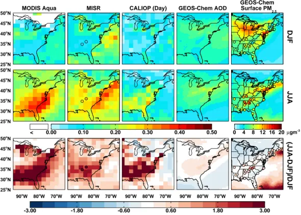
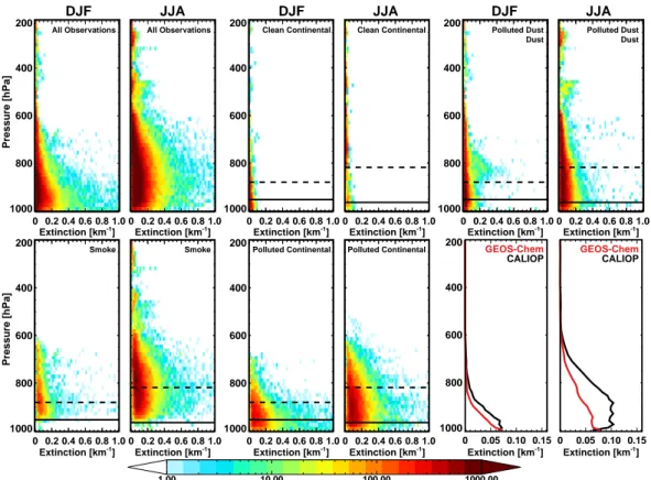
25oN 30o N 35o N 40o N 45o N 50o N 25o N 30o N 35o N 40o N 45oN 50oN < 0.00 0.10 0.20 0.30 0.40 0.50 0 4 8 12 16 20 25o N 30o N 35oN 40oN 45oN 50oN 90oW 80oW 70oW 90oW 80oW 70oW 90oW 80oW 70oW 90oW 80oW 70oW 90oW 80oW 70oW -3.00 -1.80 -0.60 0.60 1.80 3.00 MODIS Aqua MISR CALIOP (Day) GEOS-Chem AOD
GEOS-Chem Surface PM 2.5 DJF JJA (JJA-DJF)/DJF µgm-3
Fig. 1. Seasonally averaged total column AOD for winter (DJF, top row) and summer (JJA, middle row) for December 2006–August 2009
as observed by MODIS (column 1), MISR (column 2), and CALIOP (daytime, column 3) gridded to 2◦×2.5◦and compared to simulated
AOD from GEOS-Chem (column 4). Concentrations of surface PM2.5simulated by GEOS-Chem are overlaid with concentrations measured
at IMPROVE and SEARCH network sites (circles) in column 5. Bottom row shows the relative enhancement of summer over winter for observed and simulated AOD and surface concentrations. Average AOD observed at the University of Alabama, Huntsville, and Walker Branch AERONET sites for 2008–2009 is overlaid (circles) on the MISR maps.
from a tapered element oscillating microbalance (TEOM) to characterize the diurnal variability.
All eight of the SEARCH sites and several IMPROVE sites are co-located with nephelometers, which provide mea-surements of ambient relative humidity (RH). For com-parisons of vertical profiles of RH, we also use ground based soundings from 8 National Oceanic and Atmo-spheric Administration (NOAA) sites (http://weather.uwyo. edu/upperair/sounding.html). Locations of these IMPROVE, SEARCH, and NOAA sounding sites are shown in Figs. 1 and 4.
2.3 GEOS-Chem
We use v9.01.01 of the GEOS-Chem chemical transport model, driven by GEOS-5 meteorology, in the nested grid configuration over North America (0.5◦×0.667◦ horizon-tal resolution). The GEOS-Chem aerosol simulation includes sulfate, nitrate, ammonium (Park et al., 2004), primary car-bonaceous aerosols (Park et al., 2003), dust (Fairlie et al., 2007; Ridley et al., 2012), sea salt (Alexander et al., 2005), and secondary organic aerosols (SOA) (Henze et al., 2008). Aerosols and gases are removed by both wet and dry
deposi-tion in the model. The wet deposideposi-tion scheme includes scav-enging in convective updrafts, rainout and washout (Liu et al., 2001), while dry deposition of gases and aerosols is de-pendent on surface characteristics and meteorological con-ditions (Wesely, 1989; Wang et al., 1998). The EPA NEI99 inventory (scaled to be year-specific) is used for most anthro-pogenic and biofuel emissions over the USA (Hudman et al., 2007, 2008); however, anthropogenic emissions of black and organic carbon follow Cooke et al. (1999) with the seasonal-ity from Park et al. (2003). Biogenic VOC emissions are cal-culated interactively using the Model of Emissions of Gases and Aerosols from Nature (MEGAN) (Guenther et al., 2006), while year-specific biomass burning is specified according to the Global Fire Emissions Database (GFED2) inventory (van der Werf et al., 2006). We implement a fix for artificially low nighttime boundary layer heights in the GEOS-5 product as well as a 25 % reduction in the HNO3concentrations, both
of which improve comparisons with surface nitrate observa-tions in the United States as described by Heald et al. (2012). We calculate surface PM2.5 in the model by combining
sulfate, nitrate, ammonium, elemental carbon, organic matter (organic carbon scaled by a factor of 1.8 to account for to-tal organic matter, consistent with IMPROVE and SEARCH
Table 1. Mass extinction efficiency values used in GEOS-Chem for
sulfate aerosols at given relative humidity values.
Relative Humidity Mass Extinction Efficiency
(%) (m2g−1) 0 2.24 50 6.12 70 8.90 80 11.90 90 19.09 95 32.75 99 104
measurements), fine dust, and accumulation mode sea salt concentrations in the lowest grid box. For comparison with IMPROVE and SEARCH daily PM2.5 measurements, we
compute 24 h averages and sample the data to site locations and measurement days.
Aerosol optical depth in the model is calculated for a spe-cific wavelength using the extinction efficiency (Qext), the
column mass loading (M), effective radius (reff), and particle
mass density (ρ) such that the AOD (τ ) is calculated by the following equation (Tegen and Lacis, 1996):
τ =3QextM 4reffρ
=αM (1)
The aerosol mass extinction efficiency (α) is calculated with Mie code based on wavelength-resolved optical and size parameters at 7 relative humidity values (0, 50, 70, 80, 90, 95 and 99 %) for various aerosol types from the Global Aerosol Data Set (GADS) (Koepke et al., 1997), with recent updates based on Drury et al. (2010), Jaegl´e et al. (2010), and Ridley et al. (2012). The extinction efficiency for each grid box is calculated from local relative humidity conditions (Martin et al., 2003). In order to determine whether the observed sea-sonality in AOD can be attributed to changes in mass loading or mass extinction efficiency, we explore the sensitivity of the mass extinction efficiency to the observed seasonal changes in relative humidity (Sect. 3.2). For this purpose, we use the properties of sulfate aerosol (Table 1), which exhibits the strongest relationship with relative humidity (i.e., the largest hygroscopicity).
3 Results
3.1 Seasonality in AOD and surface concentrations
We mimic the seasonal AOD comparisons of Goldstein et al. (2009) in Fig. 1 for 2007–2009 using observations from MODIS Aqua, MISR, and CALIOP. Figure 1 also shows the seasonal mean AOD measured by ground-based sun pho-tometers at two AERONET sites in the SEUS.
Figure 1 shows that observed summertime AOD is con-sistently higher than wintertime values in the SEUS by a
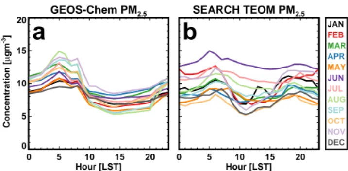
GEOS-Chem PM2.5 0 5 10 15 20 Hour [LST] 0 5 10 15 20 Concentration [ µ gm -3] SEARCH TEOM PM2.5 0 5 10 15 20 Hour [LST] JAN FEB MAR APR MAY JUN JUL AUG SEP OCT NOV DEC
a
b
Fig. 2. Diurnal cycles of monthly mean PM2.5 concentrations as
simulated by GEOS-Chem (a) and as measured by TEOM filters at SEARCH network sites (b), color-coded by month in 2009 over which the averaging was done.
factor of 2–3. This is consistent with Alston et al. (2012), who find a threefold increase in summertime AOD over win-tertime, although they use a finer resolution product and therefore show greater spatial variability. The magnitude of both the seasonal mean and the relative enhancement differs among instruments as shown in the figure, but is spatially consistent. Similar summertime enhancements are reported at AERONET sites in 2008–2009. Furthermore, AOD mea-surements at the two AERONET sites show little variability during daylight hours (< 20 % in summertime) and suggest that this enhancement is consistent throughout the day. Four independent observations, made with four different measure-ment techniques, all indicate a large regional enhancemeasure-ment in summertime AOD.
We contrast these observations with the GEOS-Chem chemical transport model simulation. Simulated summertime enhancements in AOD through the Eastern US range from 15–40 %. While the model does show a summertime maxi-mum in AOD over the Ohio River Valley and Northeastern US associated with increases in sulfate via SO2 oxidation
(Chin et al., 2000) and stagnation events, it does not repro-duce the strong observed seasonality in column AOD over the SEUS.
The fourth column of Fig. 1 shows the GEOS-Chem sim-ulated surface concentrations of PM2.5 overlaid with
ob-servations from the SEARCH and IMPROVE networks. Comparison with surface observations indicates that GEOS-Chem generally captures the spatial, seasonal, and diurnal (Fig. 2) variation of PM2.5 in the Eastern US, as will be
discussed in further sections and consistent with previous studies (e.g., Heald et al., 2012; Leibensperger et al., 2012). However, Fig. 1 shows that the measured surface concentra-tions exhibit only a fraction of the seasonality in the column AOD observed by the satellite instruments, suggesting that changes in surface concentrations do not dictate the season-ality observed in AOD. This is in agreement with Alston et al. (2012), who show that the summertime enhancement in surface PM2.5 in Georgia is considerably less than the
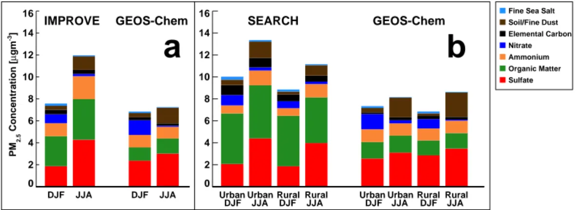
0 2 4 6 8 10 12 14 16 DJF JJA DJF JJA 0 2 4 6 8 10 12 14 16
Urban Urban Rural Rural Urban Urban Rural Rural
PM 2.5 Concentration [ µ gm -3]
IMPROVE GEOS-Chem SEARCH GEOS-Chem
DJF JJA DJF JJA DJF JJA DJF JJA
a
b
Fine Sea Salt Soil/Fine Dust Elemental Carbon Nitrate Ammonium Organic Matter Sulfate
Fig. 3. Mean seasonally averaged surface mass concentrations of PM2.5(a) observed at the 13 IMPROVE network sites in the SEUS and as
simulated by GEOS-Chem (sampled to the IMPROVE sampling days and corresponding model grid boxes). (b) Same as (a) for SEARCH network sites. All data are for December 2006–2009, except for SEARCH sea salt, which only uses data from 2009.
AOD enhancement over the region. This presents an intrigu-ing disconnect between surface and column measurements of aerosol loading in the SEUS.
In Fig. 3, we explore the chemical composition of sur-face PM2.5 over the SEUS in winter and in summer.
Over-all, the model captures the chemical speciation and the sea-sonality of IMPROVE surface concentrations in the region (Fig. 3a), but somewhat underestimates the observed sum-mertime enhancement (mean PM2.5concentration is ∼ 55 %
greater in the summertime). The observed surface seasonality is mainly due to inorganic species. Both observed and simu-lated nitrate concentrations are higher in the wintertime, con-sistent with more favorable formation of ammonium nitrate at cooler temperatures, while the increase in observed sum-mertime sulfate is the result of enhanced SO2oxidation (Chin
et al., 2000). The model simulation underestimates the dou-bling in sulfate concentrations from winter to summer seen at IMPROVE sites (specifically the Appalachian sites), but does capture the summertime enhancement associated with dust transport from North Africa (Ridley et al., 2012).
Observed OM at IMPROVE sites in the SEUS is con-sistently ∼ 2–4 µgm−3, making up less than 35 % of mean observed PM2.5, consistent with the analysis of Hand
et al. (2012). Zhang et al. (2012a) find slightly higher OM/PM2.5fractions (40–50 %) in urban areas in the SEUS;
however, when biomass burning events are removed, the fraction of water-soluble OM/PM2.5 that they observe is
re-duced to ∼ 25 %. GEOS-Chem underpredicts OM concentra-tions by about a factor of two, consistent with other regions of the world (Heald et al., 2011). However, the magnitude of OM seasonality is similar between the observations and model with very little variation in OM throughout the year (a 35 % increase in summer over winter), in agreement with values reported by Zhang et al. (2012a). The seasonality in OM (and consequently PM2.5)might be enhanced if we used
a varying OM/OC ratio, as studies have shown that the ratio
is greater in the summer than in the winter (e.g., Simon et al., 2011). However, the ratio would be applied to both the model simulation and observations, and, as GEOS-Chem is already able to simulate the OM seasonality, would therefore not explain the model discrepancy. We also compare these OM concentrations and seasonality with IMPROVE sites in the Northeastern US, where there is less of an increase in summertime AOD, and find similar values at the surface.
Observations from the SEARCH network show less sea-sonal variability in PM2.5than the IMPROVE sites, as shown
in Fig. 3b, which also highlights the differences between ru-ral and urban sites. As expected, PM2.5 concentrations are
greater at urban sites and in particular sulfate and elemen-tal carbon concentrations are higher. Additionally, although GEOS-Chem is able to simulate dust concentrations and sea-sonality at IMPROVE sites, it slightly overpredicts summer-time dust at SEARCH sites, especially rural sites. There are also higher concentrations and more seasonality in the OM at urban sites, consistent with Yan et al. (2009). Overall, the OM fraction at these SEARCH sites is greater than ob-served at the IMPROVE sites (Fig. 3a). Thus the model un-derestimate of OM is also greater. However, even more so than the IMPROVE comparisons, both the SEARCH obser-vations and the simulation of concentrations at these sites show very little seasonal variation in OM at both rural and urban sites. Additionally, there is little diurnal variability in PM2.5(Fig. 2, relative standard deviation of ∼ 10 %
through-out the year), which confirms that the seasonality in surface concentrations is consistent throughout the day and that using a 24 h average PM2.5concentration rather than a 1 h average
PM2.5concentration sampled to the satellite overpass times
does not bias the comparison with satellite observations pro-vided at two snapshots.
We conclude that the seasonality in satellite AOD over the SEUS does not match the surface concentrations or more specifically organic aerosol at the surface. This weaker
34 1
Figure 4. (a) Average 2009 monthly surface RH recorded at IMPROVE and SEARCH 2
network nephelometer sites (black) using 24 hour averages (dashed line) and sampled to the 3
afternoon overpass time (solid line). These are compared with values used in GEOS-Chem 4
(red lines) sampled to observational site locations and converted to mass extinction efficiency 5
values (for sulfate aerosols, blue lines). (b) Fractional increase in surface mass extinction 6
efficiency of summer over winter simulated with GEOS-Chem and overlaid with values 7
calculated from surface RH observed at IMPROVE nephelometer (blue circles), SEARCH 8
(green circles) and sounding (black circles) sites for 2009. GEOS-Chem, SEARCH and 9
IMPROVE data are sampled for the afternoon satellite overpass time (13-15LT) and the 10
sounding data is an average from 0000 and 1200 UTC. (c) mean profile of RH measured at 11
the 8 sounding sites (black lines) at 0000 and 1200 UTC and the corresponding RH in GEOS-12
Chem (red line) sampled to the site locations and times for winter (dashed) and summer 13
(solid) 2009. 14
15
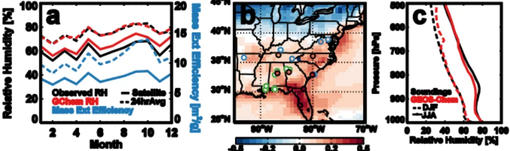
Fig. 4. (a) Average 2009 monthly surface RH recorded at IMPROVE and SEARCH network nephelometer sites (black) using 24 h averages
(dashed line) and sampled to the afternoon overpass time (solid line). These are compared with values used in GEOS-Chem (red lines) sampled to observational site locations and converted to mass extinction efficiency values (for sulfate aerosols, blue lines). (b) Fractional increase in surface mass extinction efficiency of summer over winter simulated with GEOS-Chem and overlaid with values calculated from surface RH observed at IMPROVE nephelometer (blue circles), SEARCH (green circles) and sounding (black circles) sites for 2009. GEOS-Chem, SEARCH and IMPROVE data are sampled for the afternoon satellite overpass time (13:00–15:00 LT) and the sounding data are averages from 00:00 and 12:00 UTC. (c) Mean profile of RH measured at the 8 sounding sites (black lines) at 00:00 and 12:00 UTC and the corresponding RH in GEOS-Chem (red line) sampled to the site locations and times for winter (dashed) and summer (solid) 2009.
correlation between column AOD and PM2.5(R = 0.2–0.31
for daily matched pairs across the region) in the SEUS con-trasts other regions where previous studies have found a strong correlation between satellite-observed column AOD and surface concentrations throughout the year (R = 0.39– 0.9, e.g., Engel-Cox et al., 2004; Al-Saadi et al., 2005; van Donkelaar et al., 2006; Paciorek and Liu, 2009; Zhang et al., 2009; van Donkelaar et al., 2010). These previous stud-ies note that discrepancstud-ies often arise in comparing surface concentrations and column AOD due to inaccurate assump-tions or lack of information about the hygroscopicity of the aerosols, the composition, size distributions, the vertical dis-tribution of aerosols, the presence of transported aerosols above the surface layer, and the meteorological environment, especially with regards to clouds. Correlations are highest when the aerosol is near the surface, uniformly mixed, rela-tive humidity is moderate, and coarse mode aerosol fraction is small (Al-Saadi et al., 2005; van Donkelaar et al., 2006). Therefore, in the following sections we investigate several of these factors in an attempt to determine what, other than sur-face concentrations, could be driving the seasonality in AOD.
3.2 Effect of relative humidity
Changes in aerosol water uptake could play a role in the sea-sonality of AOD in the SEUS. This is briefly examined by Goldstein et al. (2009), who find that the AOD and relative humidity (RH) at a single AERONET site (Walker Branch) are only weakly correlated across seasons. We investigate this further at several locations to better represent the effect of RH on a broader region of the SEUS. In addition, given that water uptake is already included in the simulation of AOD, we explore whether there is any evidence of a bias in RH in the GEOS-5 meteorology, which could degrade the model simulation of AOD.
Hourly surface RH values used in GEOS-Chem are highly correlated with observations from the IMPROVE and SEARCH network nephelometer sites (R = 0.6–0.83 across sites and seasons), with a mean bias of less than 5 %. Corre-lations are highest during the morning and afternoon hours and degrade during the nighttime and at coastal sites (where GEOS-Chem has a low RH bias). Figure 4a demonstrates that there is little seasonality in mean surface RH in the SEUS, and that the model reproduces both the magnitude and consistency of RH year-round. Monthly RH values av-eraged over all the sites vary less than 10 % throughout the year at the 13:30 satellite overpass and less than 20 % when all hours are used to construct monthly means.
In order to examine the impact of these modest seasonal differences in RH on AOD, we use the optical properties ap-plied to aerosols in GEOS-Chem to convert these differences in RH to differences in aerosol mass extinction efficiency. For simplicity, we use sulfate aerosol properties, which have the highest hygroscopicity (other than NaCl, which is not a significant contributor to aerosol mass in the region) (Petters and Kreidenweis, 2007) and would be the most affected by changes in RH. At the surface, seasonal differences in mass extinction efficiency due to water uptake account for less than a 25 % increase in aerosol extinction from winter to summer over the SEUS (Fig. 4b).
The seasonality in the vertical profile of RH measured at the 8 NOAA sounding sites in the region is larger, with about a 20 % absolute increase in mean RH from winter to summer throughout the troposphere (Fig. 4c). However, the seasonal difference in aerosol extinction resulting from wa-ter uptake (40 % when integrated over the column assuming sulfate aerosol) can account for only a fraction of the 100– 300 % difference in AOD observed by the satellite instru-ments over the SEUS (Fig. 1). While this increase in sum-mertime RH is generally captured by the model (and thus re-flected in the simulated AOD seasonality), RH values in the
0 0.2 0.4 0.6 0.8 1.0 1000 800 600 400 200 0 0.2 0.4 0.6 0.8 1.0 0 0.2 0.4 0.6 0.8 1.0 1000 800 600 400 200 0 0.2 0.4 0.6 0.8 1.0 0 0.2 0.4 0.6 0.8 1.0 1000 800 600 400 200 0 0.2 0.4 0.6 0.8 1.0 0 0.2 0.4 0.6 0.8 1.0 1000 800 600 400 200 0 0.2 0.4 0.6 0.8 1.0 0 0.2 0.4 0.6 0.8 1.0 1000 800 600 400 200 0 0.2 0.4 0.6 0.8 1.0 0 0.05 0.10 0.15 1000 800 600 400 200 0 0.05 0.10 0.15
All Observations Clean Continental Polluted Dust
Dust
Smoke Polluted Continental GEOS-Chem
CALIOP
Extinction [km-1] Extinction [km-1] Extinction [km-1] Extinction [km-1] Extinction [km-1] Extinction [km-1]
All Observations Clean Continental Polluted Dust
Dust
Smoke Polluted Continental GEOS-Chem
CALIOP Extinction [km-1 ] Extinction [km-1 ] Extinction [km-1 ] Extinction [km-1 ] Extinction [km-1 ] Extinction [km-1 ] Pressure [hPa] Pressure [hPa] 1.00 10.00 100.00 1000.00
DJF JJA DJF JJA DJF JJA
Fig. 5. Density plots of all nighttime aerosol extinction values observed by CALIOP for winter and summer seasons of 2007–2009 over the
SEUS (30.5–37.5◦N and 90–81.5◦W), classified by aerosol type. The color denotes the number of observations with given extinction values
at a given altitude. There are ∼ 70 000 extinction values for the winter and ∼ 200 000 for the summer from December 2006–2009, including values below the detection limit. Panels 1 and 2 show observations with all aerosol types noted, and panels 3–10 separate values based on aerosol type, with seasonally averaged boundary layer heights from GEOS-Chem for nighttime (solid black horizontal lines) and daytime (dashed lines) overlaid. Bottom right panels show average aerosol extinction profiles as observed by CALIOP (black) and the corresponding profiles simulated by GEOS-Chem and sampled to the CALIOP overpasses (red) for the two seasons applying detection limits as in Ford and Heald (2012).
lower troposphere (900–700 hPa) are slightly underestimated in summertime (< 5 %). This translates to a 5–12 % under-estimate in sulfate extinction efficiency in GEOS-Chem at these altitudes; however, the effect is likely to be more mod-est for the mix of ambient aerosol with lower hygroscopicity. Therefore, aerosol water uptake cannot explain the observed seasonality in AOD, nor can biases in RH explain the model underestimate of this seasonality.
Although we only show the sensitivity of the mass ex-tinction efficiency to RH here, we also note that changes to the aerosol size distribution not accounted for in the model could impact the observed AOD. Heald et al. (2010) use Mie code to estimate that uncertainty in mass extinction ef-ficiency associated with the size of OM (associated with a doubling or halving of the assumed mean geometric ra-dius and varying the geometric standard deviation from val-ues of 1.4 to 1.8) is ∼ 50 %. Therefore, a seasonal shift to-wards larger particles in summertime could account for some of the model–measurement discrepancy. However, measure-ments of the geometric mean diameters for ambient
SOA-dominated aerosol and fresh smoke are similar (Levin et al., 2009, 2010). Additionally, the fraction of total AOD ac-counted for by organics in the model is on average less than 15 % in the summertime, and substantial seasonal changes in the size of inorganic aerosol are less likely (e.g., Stanier et al., 2004; Zhang et al., 2008), so it is unlikely that shifts in the fine aerosol size distribution are a dominant source of model error.
3.3 The vertical profile of aerosol
The lack of strong seasonality in surface aerosol concen-trations and aerosol water content throughout the vertical column suggests that summertime increases in AOD over the SEUS must be associated with an increase in aerosol mass above the surface layer that is not accounted for in GEOS-Chem, potentially consistent with the hypothesis of Goldstein et al. (2009), which suggests a missing source of aerosols aloft.
Winter and summer vertical distributions of all the night-time aerosol extinction values reported by CALIOP for three years (2007–2009) over the SEUS are shown in Fig. 5. Sep-arating profiles based on aerosol type indicates broadly what sources are likely to contribute to the mass loading in each season, although the CALIOP algorithm is based on physi-cal properties and does not distinguish aerosol by chemiphysi-cal composition.
Figure 5 shows that there are larger aerosol extinction ob-servations at higher altitudes during the summer months. There is little seasonal difference in GEOS-5 nighttime boundary layer height (coincident with CALIOP measure-ments), but the deeper daytime mixed layers in summer may vertically distribute aerosol to higher altitudes. We investi-gate the impact of the mixing heights on the vertical profile in the next section.
In the final panels of Fig. 5, we compare the average nighttime profiles of aerosol extinction observed over the region by CALIOP with the average profile simulated by GEOS-Chem. First, these profiles confirm that the mean ob-served extinction profile over the SEUS is higher in the sum-mer than in winter. The integrated mean AOD from these profiles increases more than threefold from winter to sum-mer (0.07 to 0.25), consistent with the picture presented in Fig. 1. Second, these profiles demonstrate that the model un-derestimate of summertime AOD shown in Fig. 1 is asso-ciated with above-surface aerosols. The simulated and ob-served profile shapes are similar in the wintertime, but the model greatly underpredicts aerosol extinction above the sur-face layer in summer. While there might be a bias in the CALIOP measurements near the surface due to interference of clouds, lower sensitivity, and/or inclusion of clear air retrievals below aerosol layers (Winker et al., 2013), sur-face extinction values are generally reproduced by the model throughout the year, consistent with our PM2.5surface
com-parisons in Figs. 1 and 3. Additionally, the retrieval sen-sitivity of CALIOP increases with altitude (Winker et al., 2009), and Sheridan et al. (2012) suggest that if there is a bias in the free troposphere, it is a low bias (particularly un-der cloud-free conditions, as shown here), which suggests that the discrepancy in extinction above the surface layer be-tween the simulated and measured profile is unlikely to be due to systematic observational errors.
Mean summertime AOD calculated by integrating the model profile in Fig. 5 is 0.12, less than half the mean CALIOP values. While these profiles do not suggest that there is a distinct lofted layer of aerosol, they do indicate that the seasonality in AOD is primarily associated with an increase in aerosol mass above the surface layer in the lower troposphere (below 700 hPa), which is not captured by the GEOS-Chem model. This discrepancy is inconsistent with Heald et al. (2011), who show that the GEOS-Chem model generally captures the profiles of sulfate and organic aerosol in the Northern Hemisphere, even when concentrations are significantly underestimated.
We distinguish these CALIOP profiles by the observed aerosol types to understand the source of these aerosols, and Fig. 5 shows that the majority of aerosols observed in the SEUS is classified as polluted dust, polluted continental, and smoke. The maximum in dust above the boundary layer in the winter is likely due to dust transport from the Western US, while increases in the summer are associated with trans-port of African dust.
The summertime enhancement of extinction above the surface layer is predominantly associated with smoke and polluted continental aerosol types. This could indicate that aerosols from biomass burning are the cause of the seasonal difference. While previous studies have shown that biomass burning in the SEUS generally peaks in late winter and early spring (Zeng et al., 2008; Tian et al., 2009; Zhang et al., 2010), MODIS fire counts in this region almost double from winter to summer in 2007–2009. Furthermore, the GFED2 biomass burning emissions used in the model prescribe a fac-tor of 3-4 increase from winter to summer for these years. However, this is largely offset by a decrease in emissions of carbonaceous aerosols from anthropogenic sources in sum-mertime, such that increases in total emissions of carbona-ceous aerosols are modest (20–30 %). This is consistent with the seasonal changes reported in simulated surface carbona-ceous PM2.5 (Fig. 3). The contribution of OM to seasonally
averaged total AOD is less than 15 % in both summer and winter, suggesting that potential seasonal differences in OM injection heights would have little impact on the total extinc-tion profile. Near the surface, smoke aerosols appear to have little impact; however, this is likely due to the CALIOP al-gorithm, which generally requires that aerosols be in an el-evated layer in order to be classified as smoke (Omar et al., 2009) and will otherwise be classified as polluted continen-tal. Thus, aerosol identified by CALIOP as either polluted continental or smoke may be of the same chemical composi-tion and origin and may not be directly linked to fire activ-ity. However, because the same 532 nm lidar ratio is used for smoke and polluted continental aerosols, a misclassification will not bias the extinction profile.
3.4 Effect of planetary boundary layer height
One possible explanation of a large seasonal enhancement in AOD with modest change to surface PM2.5 is a
summer-time aerosol source with a coincident deepening of the mixed layer. As shown in Fig. 5, this deepening of the daytime plan-etary boundary layer (PBL) is simulated in the GEOS-Chem model, with an increase of more than 60 hPa from winter to summer on average. The CALIOP average summer profile suggests that the higher concentrations above the surface are relatively uniform over a deep layer (up to 800 hPa), which could indicate that the GEOS-Chem simulation does not mix pollutants through a deep-enough layer of the atmosphere, although we note that this altitude is similar to the mean sum-mertime PBL depths used in the model (shown in Fig. 5). If
the PBL heights used in the model are too shallow, pollu-tants could be trapped and more easily removed before being mixed upward.
The diurnal cycle of surface concentrations can provide some information about vertical mixing. For relatively con-stant emissions, surface concentrations generally increase at night with a shallow boundary layer and then, as the PBL height grows throughout the day, pollutants are diluted and surface concentrations decline. Thus, a shallow bias in sum-mertime afternoon mixed layer would reduce the diurnal variability in simulated PM2.5 concentrations. However, the
diurnal cycles of simulated and observed PM2.5at SEARCH
sites are relatively similar (Fig. 2), with observations show-ing slightly more consistency throughout the day, especially in the summer months. The observations shown here are con-sistent with Weber et al. (2003), who show that on aver-age PM2.5concentrations in Atlanta during August generally
vary less than 20 % through the day due to sulfate peaking in the afternoon while OM, elemental carbon, and nitrate and nitrate tend to peak in the early morning. Thus, while the contribution of the timing of different sources and mixing depths to the diurnal profile can be a challenge to untangle, the ability of the model to capture a relatively flat profile in surface PM2.5, as well as the overall seasonality and
compo-sition of that PM2.5(Fig. 3), provides evidence of a relatively
unbiased simulation of mixing depth.
It remains a challenge to validate the PBL heights used in the model simulation as there are several different ap-proaches used to estimate the height of the PBL, all of which can produce differing results (e.g., Berman et al., 1997). As shown in Marsik et al. (1995), various measurement systems can at some times differ on the height of the PBL over Atlanta by almost 1km. Therefore, we examine the sensitivity of the vertical profile and summertime AOD to changes in mixing depth in model simulations. We perform four simulations for summer 2009, in which (1) PBL heights are raised by 100 hPa at all hours of the day, (2) PBL heights are raised by 100 hPa only during daytime hours of 7.00 a.m. to 7.00 p.m. LT, (3) SO2 emissions in North America are doubled, and
(4) SO2emissions are doubled and the daytime PBL heights
are raised. The impact of these simulations on the average regional profile is shown in Fig. 6.
Raising the PBL for all hours of the day increases extinc-tion values throughout most of the profile, particularly at the top of the PBL, as concentrations are mixed throughout a deeper layer. However, values near the surface decrease as aerosols are mixed away from the surface into the deeper PBL, particularly at night. In the simulation where the PBL is only raised during the day, aerosol extinction values near the surface are similar to the original profile, but greater above the nighttime PBL, in the daytime residual layer. However, both of these simulations continue to substantially underpre-dict the extinction values compared to CALIOP (AOD in-creases by only 0.02 over the region), suggesting that a
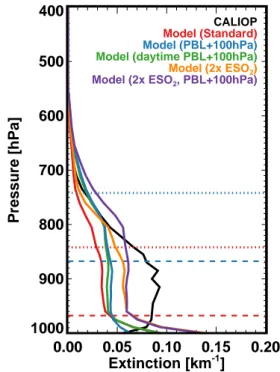
po-0.00 0.05 0.10 0.15 0.20 Extinction [km-1] 1000 900 800 700 600 500 400 Pressure [hPa] CALIOP Model (Standard) Model (PBL+100hPa) Model (daytime PBL+100hPa)
Model (2x ESO2)
Model (2x ESO2, PBL+100hPa)
Fig. 6. Aerosol extinction profiles over the SEUS for JJA 2009 as
observed by CALIOP (black) and as simulated by GEOS-Chem with original PBL heights (red), PBL heights raised by 100 hPa at all hours (blue), raised by 100 hPa during daytime hours (green),
doubled SO2emissions (orange), and doubled SO2emissions and
PBL heights raised during daytime hours (purple). Average PBL heights are shown in red for original simulation and blue for simu-lations with raised PBL heights, with dashed lines for nighttime and dotted lines for daytime.
tential bias in the PBL height would not be enough to explain the discrepancy in AOD.
Finally, we verify whether the aerosol profile measured by CALIOP is consistent with an increase in existing sources. We test increasing the sources of sulfate, which would be consistent with both the surface underestimate shown in Fig. 3 as well as the possibility of formation aloft via in-cloud processing. The profiles in Fig. 6 demonstrate that dou-bling SO2 emissions effectively scales up the entire
simu-lated profile, but in doing so significantly degrades the com-parison with both CALIOP and the speciated surface concen-trations (not shown). Simultaneously increasing the daytime PBL heights produces virtually the same profile, but pro-duces an overestimate of observed aerosol extinction from 800–700 hPa. We therefore conclude that an increase in mix-ing depth, with or without a coincident increase in an ex-isting aerosol source, cannot explain the observed CALIOP profile. This implies that the underestimate in aerosol mass aloft is due to an additional above-surface source. Using the average summertime mass extinction efficiency and the dif-ference between the satellite-estimated and simulated extinc-tion profile, we roughly estimate that this addiextinc-tional source is
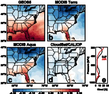
Fig. 7. Differences (summer–winter) between average cloud
frac-tion for 2006–2009 (a) from GEOS-5 sampled to afternoon over-pass, (b) observed by MODIS onboard Terra and (c) Aqua, and
(d) observed by CloudSat/CALIOP. Black outline shows region for
profiles of average cloud fraction over the SEUS for winter (black) and summer (red) observed by CloudSat/CALIOP in 2009 shown in panel (e).
equivalent to three times the current sulfate mass (above the surface only).
4 Discussion
Satellite observations show a strong summertime enhance-ment in AOD over the SEUS, previously linked with biogenic activity, which is not observed in surface PM2.5
concentra-tions. By determining here that there is little agreement be-tween surface concentrations and column AOD in the South-eastern US, we surmise that changes in surface mass concen-trations do not control the seasonality of AOD in the region. Furthermore, the GEOS-Chem model generally captures ob-served surface concentrations (with the exception of a mod-est undermod-estimate of summertime sulfate and year-round un-derestimate of OA), but it does not reproduce the observed AOD seasonality, indicating an underestimation of aerosol extinction above the surface layer in the model. We show that neither a bias in model RH (and hence aerosol water uptake) nor summertime mixing depths can explain this discrepancy. Zhang et al. (2012b) show that GEOS-Chem reproduces wet deposition measurements in the US. This suggests that this discrepancy is also not due to a bias in aerosol removal but rather a missing source of aerosol above the surface layer.
CALIOP measurements provide additional evidence of aerosol production above the surface; however, our inter-pretation is limited by the lack of aerosol chemical
specia-tion. Ervens et al. (2011) suggest that in regions where there are large biogenic VOC and anthropogenic emissions, high RH, and cloudiness, yields from aqueous formation of SOA can be significant. Carlton et al. (2008) show that including SOA formation through cloud processing modestly improves model simulations of airborne OA observations in the North-eastern US. Sooroshian et al. (2007) also observe elevated organic aerosol layers above clouds during field campaigns over Texas and California due to the formation of organic acids from aqueous phase reactions, which subsequently un-dergo droplet evaporation. Cloudy conditions as well as en-hanced oxidant concentrations in summertime could also augment sulfate production, which we show is moderately underestimated at the surface in summertime in our simula-tion. It has also been suggested that including reactions of stabilized Criegee intermediates with sulfur dioxide in mod-els can produce a 10–25 % increase in sulfuric acid (H2SO4)
annually and a 100 % increase in July (Pierce et al., 2013). GEOS-5 meteorology does show higher cloud fractions over the SEUS in the summer compared to the winter, which is corroborated by observations from MODIS Aqua and Terra (Fig. 7). If clouds are indeed serving as a medium for chemical production, this could explain the increased aerosol loading above the surface layer that is seen in the cloud-free CALIOP profiles shown here. However, observations from the CloudSat Cloud Profiling Radar suggest that mid- to low troposphere cloud cover is highest in the region in winter (Fig. 7). Furthermore, we see no evidence of a correlation in daily cloud optical depth and aerosol extinction reported by CloudSat and CALIOP over the region. These conflicting characterizations of cloud seasonality and a lack of corre-spondence between cloud cover and aerosol loading suggest that cloud liquid water may not be the limiting factor in sum-mertime aerosol production, but rather that the oxidation of biogenic VOCs, whose emission peaks in summertime, is re-quired to explain the observed aerosol enhancement above the surface layer.
It is vital, therefore, to have in situ vertical measurements of aerosol composition in order to fully investigate this hy-pothesis of increased aqueous aerosol production aloft and determine whether it is organic or inorganic in nature. The SAS campaign aircraft data will be critical for resolving this issue and determining the aerosol characteristics in the SEUS, thus enabling a better prediction of how aerosol in this region is likely to evolve.
Acknowledgements. This work was supported by the National
Science Foundation (ATM-0929282). We thank the satellite (MODIS, MISR, CALIOP, CloudSat) and in situ measurement teams (AERONET, IMPROVE, SEARCH).
References
Alexander, B., Park, R. J., Jacob, D. J., Li, Q. B., Yantosca, R. M., Savarino, J., Lee, C. C. W., and Thiemens, M. H.: Sulfate for-mation in sea-salt aerosols: Constraints from oxygen isotopes, J. Geophys. Res., 110, D10307, doi:10.1029/2004JD005659, 2005. Al-Saadi, J., Szykman, J., Pierce, R. B., Kittaka, C., Neil, D., Chu, D. A., Remer, L., Gumley, L., Prins, E., Weinstock, L., MacDon-ald, C., Wayland, R., Dimmick, F., and Fishman, J.: Improving National Air Quality Forecasts with Satellite Aerosol Observa-tions, B. Am. Meteorol. Soc., 86, 1249–1261, 2005.
Alston, E. J., Sokolik, I. N., and Kalashnikova, O. V.: Characteriza-tion of atmospheric aerosol in the US Southeast from ground-and space-based measurements over the past decade, Atmos. Meas. Tech., 5, 1667–1682, 2012,
http://www.atmos-meas-tech.net/5/1667/2012/.
Berman, S., Ku, J.-Y., Zhang, J., and Rao, S. T.: Uncertainties in estimating the mixing depth-comparing three mixing-depth mod-els with profiler measurements, Atmos. Environ., 31, 3023–3039, 1997.
Carlton, A. G., Turpin, B. J., Altieri, K. E., Seitzinger, S. P., Mathur, R., Roselle, S. J., and Weber, R. J.: CMAQ model performance enhanced when in-cloud secondary organic aerosol is included: comprisons of organic carbon predictions with measurements, Environ. Sci. Technol., 42, 8798–8802, 2008.
Chin, M., Savoie, D. L., Huebert, B. J., Bandy, A. R., Thornton, D. C., Bates, T. S., Quinn, P. K., Saltzman, E. S., and De Bruyn, W. J.: Atmospheric sulfur cycle simulated in the global model GO-CART: Comparison with field observations and regional budgets, J. Geophys. Res., 105, 24689–24712, 2000.
Cooke, W. F., Liousse, C., Cachier, H., and Feichter, J.:
Con-struction of a 1◦×1◦fossil fuel emission data set for
carbona-ceous aerosol and implementation and radiative impact in the ECHAM4 model, J. Geophys. Res., 104, 22137–22,162, 1999. Diner, D. J., Braswell, B. H., Davies, R., Gobron, N., Hu, J., Jun,
Y., Kahn, R. A., Knyazikhin, Y., Loeb, N., Muller, J.-P., Nolin, A. W., Pinty, B., Schaaf, C., Seiz, G., and Stroeve, J.: The value of multiangle measurements for retrievein structurally and radia-tively consistent properties of clouds, aerosols, and surfaces, Re-mote Sens. Environ., 97, 495–518, 2005.
Drury, E., Jacob, D. J., Spurr, R. J. D., Wang, J., Shinozuka, Y., An-derson, B. E., Clarke, A. D., Dibb, J., McNaughton, C., and We-ber, R.: Synthesis of satellite (MODIS), aircraft (ICARTT), and surface (IMPROVE, EPA-AQS, AERONET) aerosol observa-tions over eastern North America to improve MODIS aerosol re-trievals and constrain surface aerosol concentrations and sources, J. Geophys. Res., 115, D14204, doi:10.1029/2009JD012629, 2010.
Duncan, B. N., Martin, R. V., Staudt, A. C., Yevich, R., and Logan, J. A.: Interannual and seasonal variability of biomass burning emissions constrained by satellite observations, J. Geophys. Res., 108, D2, doi:10.1029/2002JD002378, 4100, 2003.
Edgerton, E. S., Hartsell, B. E., Saylor, R. D., Jansen, J. J., Hansen, D. A., and Hidy, G. M.: The Southeastern Aerosol Research and Characterization Study: Part II. Filter-based measurements of fine and coarse particulate matter mass and composition, J. Air Waste Manag. Assoc., 55, 1527–1542, 2005.
Edgerton, E. S., Hartsell, B. E., Saylor, R. D., Jansen, J. J., Hansen, D. A., and Hidy, G. M.: The Southeastern Aerosol Research and Characterization Study, Part 3: continuous measurements of fine
particulate matter mass and composition, J. Air Waste Manag. Assoc., 56, 1325–1341, 2006.
Engel-Cox, J. A., Hoff, R. M., Rogers, R., Dimmick, F., Rush, A. C., Szykman, J. J., Al-Saadi, J., Chu, D. A., and Zell, E. R.: Inte-grating lidar and satellite optical depth with ambient monitoring for 3-dimensional particulate characterization, Atmos. Environ., 40, 8056–8067, 2006.
Ervens, B., Turpin, B. J., and Weber, R. J.: Secondary or-ganic aerosol formation in cloud droplets and aqueous parti-cles (aqSOA): a review of laboratory, field and model stud-ies, Atmos. Chem. Phys., 11, 11069–11102, doi:10.5194/acp-11-11069-2011, 2011.
Fairlie, D. T., Jacob, D. J., and Park, R. J.: The impact of transpacific transport of mineral dust in the United States, Atmos. Environ., 41, 1251–1266, 2007.
Ford, B. and Heald, C. L.: An A-train and model perspec-tive on the vertical distribution of aerosols and CO in the Northern Hemisphere, J. Geophys. Res., 117, D06211, doi:10.1029/2011JD016977, 2012.
Goldstein, A. H., Koven, C. D., Heald, C. L., and Fung, I. Y.: Bio-genic carbon and anthropoBio-genic pollutants combine to form a cooling haze over the southeastern United States, PNAS, 106, 8835–8840, 2009.
Guenther, A., Karl, T., Harley, P., Wiedinmyer, C., Palmer, P. I., and Geron, C.: Estimates of global terrestrial isoprene emissions using MEGAN (Model of Emissions of Gases and Aerosols from Nature), Atmos. Chem. Phys., 6, 3181–3210, doi:10.5194/acp-6-3181-2006, 2006.
Hallquist, ˚A. M., Jerksj¨o, M., Fallgren, H., Westerlund, J., and
Sj¨odin, ˚A.: Particle and gaseous emissions from individual
diesel and CNG buses, Atmos. Chem. Phys., 13, 5337–5350, doi:10.5194/acp-13-5337-2013, 2013.
Hand, J. L., Schichtel, B. A., Pitchford, M., Malm, W. C., and Frank, N. H.: Seasonal composition of remote and urban fine particu-late matter in the United States, J. Geophys. Res., 117, D05209, doi:10.1029/2011JD017122, 2012.
Hansen, D. A., Edgerton, E. S., Hartsell, B. E., Jansen, J. J., Kan-dasamy, N., Hidy, G. M., and Blanchard, C. L.: The Southeastern Aerosol Research and Characterization Study: part 1 – Overview, J. Air Waste Manag. Assoc., 53, 1460–1471, 2003.
Heald, C. L., Wilkinson, M. J., Monson, R. K., Alo, C. A., Wang, G., and Guenther, A.: Response of isoprene emission to ambient CO2 changes and implications for global budgets, Glob. Change Biol., 15, 1127–1140, 2009.
Heald, C. L., Ridley, D. A., Kreidenweis, S. M., and Drury,
E. E.: Satellite observations cap the atmospheric
or-ganic aerosol budget, Geophys. Res. Lett., 37, L24808, doi:10.1029/2010GL045095, 2010.
Heald, C. L., Coe, H., Jimenez, J. L., Weber, R. J., Bahreini, R., Middlebrook, A. M., Russell, L. M., Jolleys, M., Fu, T.-M., Al-lan, J. D., Bower, K. N., Capes, G., Crosier, J., Morgan, W. T., Robinson, N. H., Williams, P. I., Cubison, M. J., DeCarlo, P. F., and Dunlea, E. J.: Exploring the vertical profile of atmo-spheric organic aerosol: comparing 17 aircraft field campaigns with a global model, Atmos. Chem. Phys., 11, 12673–12696, doi:10.5194/acp-11-12673-2011, 2011.
Heald, C. L., Collett Jr., J. L., Lee, T., Benedict, K.B., Schwandner, F. M., Li, Y., Clarisse, L., Hurtmans, D. R., Van Damme, M., Clerbaux, C., Coheur, P.-F., Philip, S., Martin, R. V., and Pye, H.
O. T.: Atmospheric ammonia and particulate inorganic nitrogen over the United States, Atmos. Chem. Phys., 12, 10295–10312, doi:10.5194/acp-12-10295-2012, 2012.
Henze, D. K., Seinfeld, J. H., Ng, N. L., Kroll, J. H., Fu, T.-M., Jacob, D. J., and Heald, C. L.: Global modeling of secondary organic aerosol formation from aromatic hydrocarbons: high-vs. low-yield pathways, Atmos. Chem. Phys., 8, 2405–2420, doi:10.5194/acp-8-2405-2008, 2008.
Holben, B. N., Eck, T. F., Slutsker, I., Tanr´e, D., Buis, J. P., Setzer, A., Vermote, E., Reagan, J. A., Kaufman, Y. J., Nakajima, T., Lavenu, F., Jankowiak, I., and Smirnov, A.: AERONET – A Fed-erated Instrument Network and Data Archive for Aerosol Char-acterization, Remote Sens. Environ., 66, 1–16, 1998.
Hoyle, C. R., Boy, M., Donahue, N. M., Fry, J. L., Glasius, M., Guenther, A., Hallar, A. G., Huff Hartz, K., Petters, M. D., Pet¨aj¨a, T., Rosenoern, T., and Sullivan, A. P.: A review of the anthro-pogenic influence on biogenic secondary organic aerosol, Atmos. Chem. Phys., 11, 321–343, doi:10.5194/acp-11-321-2011, 2011. Hudman, R. C., Jacob, D. J., Turquety, S., Leibensperger, E. M., Murray, L. T., Wu, S., Gilliland, A. B., Avery, M., Bertram, T. H., Brune, W., Cohen, R. C., Dibb, J. E., Flocke, F. M., Fried, A., Holloway, J., Neuman, J. A., Orville, R., Perring, A., Ren, X., Sachse, G. W., Singh, H. B., Swanson, A., and Wooldridge, P. J.: Surface and lightning sources of nitrogen oxides over the United States: Magnitudes, chemical evolution, and outflow, J. Geophys. Res., 112, D12S05, doi:10.1029/2006JD007912, 2007. Hudman, R. C., Murray, L. T., Jacob, D. J., Millet, D. B.,
Tur-quety, S., Wu, S., Blake, D. R., Goldstein, A. H., Holloway, J., and Sachse, G. W.: Biogenic versus anthropogenic sources of CO in the United States, Geophys. Res. Lett., 35, L04801, doi:10.1029/2007GL032393, 2008.
Hunt, W. H., Winker, D. M., Vaughan, M. A., Powell, K. A., Lucker, P. L., and Weimer, C.: CALIPSO Lidar Description and Per-formance Assessment, J. Atmos. Ocean. Tech., 26, 1214–1228, 2009.
Jaegl´e, L., Quinn, P. K., Bates, T. S., Alexander, B., and Lin, J.-T.: Global distribution of sea salt aerosols: new constraints from in situ and remote sensing observations, Atmos. Chem. Phys., 11, 3137–3157, doi:10.5194/acp-11-3137-2011, 2011.
Koepke, P., Hess, M., Schult, I., and Shettle, E. P.: Global Aerosol Data Set, Max-Planck-Institut f¨ur Meteorologie, Hamburg, 1997. Leibensperger, E. M., Mickley, L. J., Jacob, D. J., Chen, W.-T., Se-infeld, J. H., Nenes, A., Adams, P. J., Streets, D. G., Kumar, N., and Rind, D.: Climatic effects of 1950–2050 changes in US an-thropogenic aerosols – Part 2: Climate response, Atmos. Chem. Phys., 12, 3349–3362, doi:10.5194/acp-12-3349-2012, 2012. Levin, E. J. T., Kreidenweis, S. M., McMeeking, G. R., Carrico, C.
M., Collet Jr., J. L., and Malm, W. C.: Aerosol physical, chem-ical and optchem-ical properties during the Rocky Mountain Airborne Nitrogen and Sulfur study, Atmos. Environ., 43, 1932–1939. Levin, E. J. T., McMeeking, G. R., Carrico, C. M., Mack, L.
E., Kreidenweis, S. M., Wold, C. E., Moosm¨uller, Arnott, W. P., Hao, W. M., Collet Jr., J. L., and Malm, W. C.: Biomass burning smoke aerosol poperties measured during Fire Labora-tory at Missoula Experiments (FLAME), J. Geophys. Res., 115, D18210, doi:10.1029/2009JD013601, 2010.
Lim, H.-J. and Turpin, B. J.: Origins of Primary and Secondary Or-ganic Aerosol in Atlanta:? Results of Time-Resolved Measure-ments during the Atlanta Supersite Experiment, Environ. Sci.
Technol., 36, 4489–4496, 2002.
Liu, H., Jacob, D. J., Bey, I., and Yantosca, R. M.: Constraints from 210Pb and 7Be on wet deposition and transport in a global three-dimensional chemical tracer model driven by assimilated meteo-rological fields, J. Geophys. Res., 106, 12109–12128, 2001. Malm, W. C. and Hand, J. L.: An examination of the physical and
optical properties of aerosols collected in the IMPROVE pro-gram, Atmos. Environ., 41, 3407–3427, 2007.
Malm, W. C., Sisler, J. F., Huffman, D., Eldred, R. A., and Cahill, T. A.: Spatial and seasonal trends in particle concentration and op-tical extinction in the United States, J. Geophys. Res., 99, 1347– 1370, 1994.
Mamouri, R. E., Amiridis, V., Papayannis, A., Giannakaki, E., Tsaknakis, G., and Balis, D. S.: Validation of CALIPSO space-borne-derived attenuated backscatter coefficient profiles using a ground-based lidar in Athens, Greeces, Atmos. Meas. Tech., 2, 513–522, doi:10.5194/amt-2-513-2009, 2009.
Marsik, F. J., Fischer, K. W., McDonald, T. D., and Samson, P. J.: Comparison of Methods for Estimating Mixing Height Used during the 1992 Atlanta Field Intensive, J. Appl. Meteorol., 38, 1802–1814, 1995.
Martin, R. V., Jacob, D. J., Yantosca, R. M., Chin, M., and Ginoux, P.: Global and regional decreases in tropospheric oxidants from photochemical effects of aerosols, J. Geophys. Res., 108, 4097, doi:10.1029/2002JD002622, 2003.
Martonchik, J. V., Kahn, R. A., and Diner, D. J.: Retrieval of aerosol properties over land using MISR observations, in: Satellite Aerosol Remote Sensing Over Land, edited by: Kokhanovsky, A. A. and de Leeuw, G., Springer Praxis, Berlin, 267–291, 2009. Mona, L., Pappalardo, G., Amodeo, A., D’Amico, G., Madonna, F., Boselli, A., Giunta, A., Russo, F., and Cuomo, V.: One year of CNR-IMAA multi-wavelength Raman lidar measurements in coincidence with CALIPSO overpasses: Level 1 products com-parison, Atmos. Chem. Phys., 9, 7213–7228, doi:10.5194/acp-9-7213-2009, 2009.
Omar, A. H., Won, J.-G., Winker, D., M., Yoon, S.-C., Dubovik, O., and McCormick, M. P.: Development of global aerosol models using cluster analysis of Aerosol Robotic Network (AERONET) measurements, J. Geophys. Res., 110, D10S14, doi:10.1029/2004JD004874, 2005.
Omar, A. H., Winker, D. M., Vaughan, M. A., Hu, Y., Trepte, C. R., Ferrare, R. A., Lee, K.-P., Hostetler, C. A., Kittaka, C., Rogers, R. R., Kuehn, R. E., and Liu, Z.: The CALIPSO Automated Aerosol Classification and Lidar Ratio Selection Algorithm, J. Atmos. Ocean. Tech., 26, 1994–2014, 2009.
Paciorek, C. J. and Liu, Y.: Limitatinons of Remotely Sensed Aerosol as a Spatial Proxy for Fine Particulate Matter, Environ. Health Perspect., 117, 904–909, 2009.
Park, R. J., Jacob, D. J., Chin, M., and Martin, R. V.: Sources of carbonaceous aerosols over the United States and implications for natural visibility, J. Geophys. Res., 108, 2002–3190, 2003. Park, R. J., Jacob, D. J., Field, B. D., Yantosca, R. M.,
and Chin, M.: Natural and transboundary pollution influ-ences on sulfate-nitrate-ammonium aerosols in the United States: Implications for policy, J. Geophys. Res., 109, D15204, doi:10.1029/2003JD004473, 2004.
Peltier, R. E., Sullivan, A. P., Weber, R. J., Wollny, A. G., Holloway, J. S., Brock, C. A., de Gouw, J. A., and Atlas, E. L.: No evidence for acid-catalyzed secondary organic aerosol formation in power