3-D Finite Difference Modeling for Borehole and Reservoir
Applications
Mary L. Krasovec, Daniel R. Burns, Mark E. Willis, Shihong Chi, and M. Nafi Toks¨
oz
Earth Resources Laboratory
Dept. of Earth, Atmospheric, and Planetary Sciences
Massachusetts Institute of Technology
Cambridge, MA 02139
Abstract
ERL’s in-house finite difference code (Krasovec et al., 2003) has undergone several upgrades in the past year. Most notably, a stretched grid can now be used to greatly reduce the amount of RAM memory needed by certain types of models. Improvements have been made in the GUI front end, allowing more freedom and ease in building the model, source or source array, and receiver array.
The finite difference code has contributed to several different research projects at ERL in the past year. A few of these projects, including borehole seismics, reservoir delineation, and source mechanics, are shown in this report.
Introduction
In an effort to expand the modeling tools available at ERL, we have updated a finite difference code first developed by Cheng (1994) to model seismic waves in anisotropic, viscoelastic media. The wave equation is discretized in velocity and stress on a staggered grid, is 2nd order in time and 4th order in space, and models anisotropy with up to nine elastic constants. Two types of boundary conditions can be used: those of Cerjan et al. (1987) or Higdon (1986, 1987). The method of Emmerich and Korn (1987) can be used to include attenuation in the calculations, with three relaxation frequencies, as discussed in Krasovec et al. (2003).
Originally written in Fortran, the code has been converted to MPI C to allow it to run large models on a PC cluster. A front end of Matlab graphic user interfaces (GUIs) have also been developed to make the code easier to use.
A 2D version of the code was released at ERL’s 2003 Consortium. This year, the 3D version, including the Matlab GUIs, the Matlab mex version, a standalone serial version, a parallel MPI C version, a number of accompanying Matlab scripts, a tutorial, and a manual are included in the software release.
Upgrades to the GUIs can best be experienced by going through the tutorial. This paper focuses on the output of the code as opposed to its usage. First, we show a comparison of the finite difference code to discrete wavenumber results for a 3D fluid filled borehole. Second, we show a more complicated borehole geometry: finite difference modeling results of ERL’s scaled down LWD tool. Moving away from the borehole geometry, the third example looks for shear wave splitting in synthetic micro earthquake data due to the presence of fractures in a reservoir layer. The final example shows how an empty cylindrical cavity located next to an explosion source can scatter the source energy into shear waves, a problem of interest in monitoring for the Comprehensive Test Ban Treaty.
The Stretched Grid
Some models can be made more computationally efficient by using a stretched grid. For example, borehole models need small grid elements in the borehole, because the fluid velocity is low, hence the wavelength
is short, and also because a fine grid is needed to accurately represent the curvature of the borehole wall. However, the fine grid is unnecessary in the formation, where wavelengths are longer and there may be no small scale structure.
3D borehole models routinely run at ERL would require well over 1000 Gig of memory to run without the stretched grid, but with stretching the memory is reduced to less than 8 Gig.
The variable grid is implemented by transforming the physical grid, which has variable element size, to a computational grid which is uniform. This process is described in detail in Huang (2003).
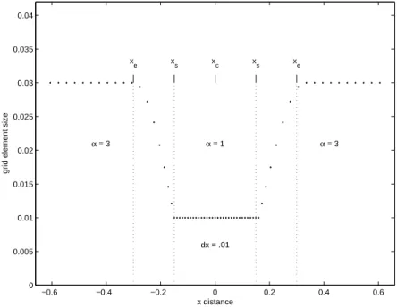
Figure 1 shows how a variable grid can be built for a borehole model, focusing on the stretching of the x axis (x, y and z are treated separately). The borehole would be centered at x=0, with a radius less than xs. In the region which includes the borehole, the grid is at its finest. In the regions from xs to xe, the grid
starts and ends its stretching. The grid stretches by a factor of α = 3.
−0.6 −0.4 −0.2 0 0.2 0.4 0.6 0 0.005 0.01 0.015 0.02 0.025 0.03 0.035 0.04 x distance
grid element size
x c xs xe x s x e α = 1 α = 3 α = 3 dx = .01
Figure 1: An example of stretched grid geometry: this grid has its finest element size, dx = .01, at xc = 0,
and two transitions. The transition to the left has xs1 = −0.15, xe1 = −0.3, α = 3. The transition to the
right has xs2= 0.15, xe2= 0.3, α = 3.
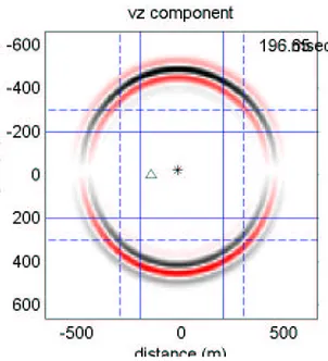
As an example of the stretched grid, a 2D model was built with stretching in both the x and z dimensions. Figure 2 shows a snapshot from the model, where the source is located in the fine grid region, shown as a black asterisk near the center of the grid. The blue lines show the region with the fine grid. Inside the solid lines, the grid is fine. Outside the dashed lines, the grid is stretched by a factor of 4. No reflection or distortion of the wavefield is apparent in the snapshot.
Figure 3 shows traces calculated tih the stretched as compared to a regular grid, which has the finest spacing with no stretching. The receiver location is plotted as a triangle in Figure 2. The amplitude of the reflection from the grid transition zone is less than 1% of the amplitude of the main pulse.
Figure 2: A snapshot of the vertical component of the wavefield from a point source on a stretched grid. The grid is fine in the region near the source, between the solid blue lines. The grid stretches by a factor of four between the solid lines and the dashed lines.
0 100 200 300
time (msecs)
regular grid variable grid
Figure 3: Wavefield recored at the receiver marked as a triangle in Figure 2. The result on a regular fine grid is shown in black, the result on the stretched grid in red.
1
Simple borehole model
A simple borehole model borrowed from Schmitt and Bouchon (1985) is used to validate the finite difference scheme. The model is a fluid filled borehole with no tool, with the geometry as shown in Figure 4. The borehole is located in a hard formation, with vp= 4800 m/s and vs= 2805 m/s, ρ = 2.4 g/cc. The fluid has
vp = 1500 m/s, the borehole radius is .12 m, and the source is a Kelly wavelet with center frequency 7500
Hz.
Figure 4: The geometry of a simple borehole model (from Schmitt and Bouchon (1985)) which is used to validate the finite difference scheme.
The source is a point source located at the center of the borehole at level z=0. The pressure wavefield is recorded at 12 levels and four lateral positions: at the center of the borehole, the edge of the borehole, and at 1/3 and 2/3 of the radius.
Figure 5 shows the output. The finite difference results show the expected characteristics: the P and S arrivals with arrive with the velocities shown in blue and redi, but are of small amplitude and difficult to see on this plot. The Stoneley wave is the single large pulse which dominates the gather at r = 8 cm. The Airy phase phase the last large amplitude arrival. i
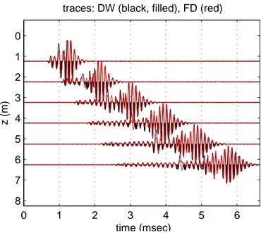
To validate the results, an in-house discrete wavenumber code was run for the receiver string located in the center of the borehole. This traces overlie the finite difference results on Figure 6.
Figure 7 shows time semblance analysis for both data sets. The first two traces are not used in the semblance calculation. The two semblance plots are very similar except for at early times and high velocities, where the finite difference inherently has no information.
1 2 3 4 5 6 0 1 2 3 4 5 6 7 z (meters) r = 0 cm 1 2 3 4 5 6 0 1 2 3 4 5 6 7 r = 8 cm 1 2 3 4 5 6 0 1 2 3 4 5 6 7 time (ms) z (meters) r = 4 cm 1 2 3 4 5 6 0 1 2 3 4 5 6 7 time (ms) r = 12 cm
Figure 5: The output from the finite difference code at a number of positions in the borehole. The first plot, for a string of receivers located at the center of the borehole, has an overlay of traces calculated by a discrete wavenumber code.
0 1 2 3 4 5 6 0 1 2 3 4 5 6 7 8 z (m) time (msec)
traces: DW (black, filled), FD (red)
Figure 6: Traces at the center of the borehole. The top plot shows the results from the finite difference code and from the discrete wavenumber method.
Figure 7: Time semblance calculations for traces shown in Figure 6. The finite difference lacks information at early times and high velocities, but otherwise matches the discrete wavenumber results well.
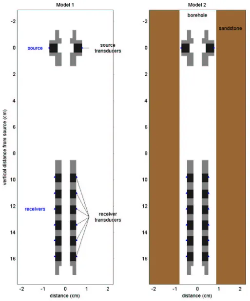
Figure 8: A vertical cross section of the model of the LWD lab tool.
2
LWD lab tool model
ERL has a scaled down LWD tool which is used in the laboratory to measure guided seismic waves in material samples. To better understand and predict lab results, a model of the LWD tool has been built for the finite difference code.
Figure 8 show a vertical cross sections of three versions of the 3D model. The tool consists of a source section, a receiver section, and a connector which is not used in these examples. Model 1 has the tool suspended in water. Model 2 has the tool in a water filled borehole in a sandstone formation.
Both models were run using a dipole source with a Kelly source time function with a center frequancy of 50 kHz. The sandstone model required about 8 Gig of Ram (as opposed to over 1000 Gig without the stretched grid!) and ran in about 4 days.
Figure 9 shows the results and analysis of the dipole response of both models. Model 1 shows energy arriving in the tool at an early time. The velocity lies below the steel velocity of 5860 mostly water waves, The time semblance analysis of Model 1 shows energy arriving at an early time with a velocity of about 5000
0.1 0.2 0.3 0.4 0.08 0.1 0.12 0.14 0.16 0.18 time (ms) z offset
NoSpacer2 dipole traces
time (ms) phase velocity (m/s) time semblance 0 0.2 0.4 2000 4000 6000 0.1 0.2 0.3 0.4 0.08 0.1 0.12 0.14 0.16 0.18 time (ms) z offset Sandstone WL dipole traces time (ms) phase velocity (m/s) time semblance 0 0.2 0.4 2000 4000 6000
Figure 9: Results and analysis for dipole source in Model 1 (left plots) and Model 2 (right plots). Black lines on all plots correspond to tool velocities, red lines are formation velocites in Model 2, and the cyan line in water velocity. Dashed lines are shear velocities, solid lines are P wave velocities. See the text for further discussion.
m/s. This lies between the tool steel and transducers velocities, at 5860 and 4158 m/s, respectively. The time semblance analysis of Model 2 shows the formation P wave arrival at 4660 m/s and guided waves arriving just below the formation shear velocity.
The traces for both cases have a great deal of energy arriving at later times. This is because the model is run with no attenuation; the source section continues to ring long after the source is done firing, and likewise waves in the receiver section reverberate with little loss of energy.
3
Shear wave splitting
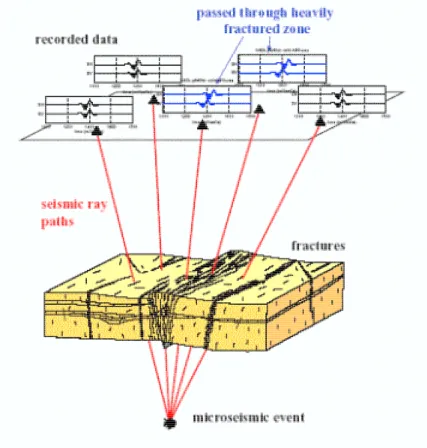
There are several projects at ERL which focus on reservoir development, and in particular the characteriza-tion of fractures in hydrocarbon and geothermal reservoirs. One phenomenon currently being investigated is shear wave splitting in microearthquakes or induced seismic event data. Figure 10 illustrates the principle.
Figure 10: Schematic of shear wave splitting effects recorded at different spatial locations in a reservoir.
When fractures are introduced into a homogeneous medium, the uniform, isotropic properties of the medium are altered and the medium properties become directionally dependent and anisotropic. When a seismic wave propagates through an anisotropic reservoir (due to aligned fractures, or non-uniform stress field) the directional variations in the shear wave velocity causes of splitting of the shear waves. The result is a relative time delay between the two polarized shear wave arrivals, with the delay being a function of the propagation path and the amount of fracturing or stress difference in the reservoir.
The size, shape, distribution and orientation of the fractures dictate the nature and magnitude of the anisotropy observed. For fractures which are small with respect to the seismic wavelength, the medium may be parameterized by a homogeneous, equivalent medium with the appropriate anisotropic parameters. For fractures which are comparable to the seismic wavelength, the discrete fractures must be modeled individually. The finite difference code be used to model both cases: either an effective anisotropic material can be used to model fine scale fracturing, or discrete fractures can be modeled as columns of highly compliant material (see Krasovec et al. (2003)).
In this example, we investigate the former case, using the model of Krasovec et al. (1998) to calculate effective medium parameters for small scale fractures in the reservoir layer. Figure 11 shows the generalized schematic of a model representing a vertically fractured hydrocarbon reservoir with a micro-earthquake located in the bottom left corner. The model was run with and without fractures in the reservoir layer.
Figure 11: generalized schematic of a model representing a vertically fractured hydrocarbon reservoir with a micro-earthquake located in the bottom left corner
Figure 12 shows horizontal components of the wavefield at 2100 meters horizontal offset from the source for three situations: for the unfractured medium, for fractures oriented parallel to the propagation direction, and for fractures oriented normal to the propagation direction. Notice the clear delay of the split shear waves on the SH component of the fractured model collected parallel to the fracture orientation (middle display). Also evident is the clear delay and quasi-shear precursor modes on the SV component of the fractured model collected normal to the fracture orientation (bottom display).
Figure 12: Shear waves from synthetic micro-earthquakes for three cases: for the unfractured medium, for fractures oriented parallel to the propagation direction, and for fractures oriented normal to the propagation direction.
4
Explosion Source Mechanics
The 3D variable grid finite difference modeling code is used to model the effect a cylindrical cavity located near an explosion source has on the radiated seismic wavefield.
Figure 13 shows a vertical snapshot of the vertical component of the velocity field at an early time. Brown lines show an outline of the cylinder with the sopuce located just to its left. Table 1 lists the model parameters. The blue lines in Figure 13 show how the grid is fine near the source to accurately model the shape of the cylinder, then stretches to be more computationally effecient in the homogenous part of the model. −60 −40 −20 0 20 40 60 80 40 60 80 100 120 140 160 x distance (m) depth (m)
vertical snapshot at 100 msecs
Figure 13: Snapshot of the divergence of the wavefield at an early time. The blue lines show the variable grid used to accurately model the cylinder, while maintaining computational effeciency elsewhere.
cylinder radius 15 meters cylinder length 30 meters source/cylinder separation 15 meters source/cylinder depth 100 meters background P-wave velocity 4000 m/s background S-wave velocity 2500 m/s background density 2.5 g/cc cylinder P-wave velocity 340 m/s cylinder density 0.2 g/cc source center frequency 20 Hz (Kelly wavelet)
Table 1: Model Parameters. The density in the cylinder had to be slightly higher than air density to stabilize the calculation.
Figures 14 and 15 show snapshots of the velocity field, without and with the cylinder. The divergence in the left column of each figure is the P-wave energy, while the curl in the right column is the S-wave energy. The presence of the cylindrical void results in an increase in scattered S-waves, and the reverberation of energy in the cylinder, visible as a small spot near the source in Figure 15, continues long after the source fires.
Figure 16 shows the vertical, radial and transverse components of the velocity field at a distance of about 1400 meters from the source. Each plot shows two traces: the top trace is without and the bottom is with the cylinder. The vertical and radial components in the top two plots show that scattering from the cylinder causes a much longer wavetrain for the P and SV phases. The cylinder also scatters energy into the SH phase, as visible in the transverse component in the bottom plot.
Figure 14: Snapshots for the model with no cylinder. On the left is the divergence of the velocity, which shows mostly P wave energy. On the right is the curl of the velocity field, which is the S wave energy due to the free surface reflection.
100 200 300 400 500 600 700 800 900 No cyl
cyl
time (msecs)
vertical component at x = 1397 meters
100 200 300 400 500 600 700 800 900
No cyl
cyl
time (msecs) radial component at x = 1397 meters
100 200 300 400 500 600 700 800 900
No cyl
cyl
time (msecs)
transverse component at x = 1397 meters
Figure 16: Recorded waveforms for a receiver at distance of 1397 meters. Each plot shows the result without (top trace) and with (bottom trace) the cylinder. The radial and transverse plots have their amplitudes scaled 5 times the scale used for the vertical component. The presence of the cylinder results in a longer wavetrain in the vertical and transverse components, and more shear wave energy in the transverse component (SH phase).
5
Conclusions
Improvements in ERL’s finite difference code, including the variable grid, have led to increased usage of the code in several fields of research at ERL. We have shown that the finite difference code yields results that meet expectations and will allow further investigation into borehole seismics, reservoir delineation, and source mechanics.
6
Acknowledgments
This work was supported by the Borehole Acoustics and Logging Consortium and the Founding Member Consortium at the Earth Resources Laboratory.
References
Cerjan, C., Kosloff, D., Kosloff, R., and Reshef, M. (1987). A nonreflecting boundary condition for discrete acoustic and elastic wave equations. Geophysics, 50(4):705–708.
Cheng, N. (1994). Borehole Wave Propagation in Isotropic and Anisotropic Media: Three-Dimensional Finite Difference Approach. PhD thesis, Massachusetts Institute of Technology.
Emmerich, H. and Korn, M. (1987). Incorporation of attenuation into time-domain computations of seismic wave fields. Geophysics, 52(9):12521264.
Higdon, R. L. (1986). Absorbing boundary conditions for difference approximations to the multi-dimensional wave equation. Mathematics of Computation, 47:437–459.
Higdon, R. L. (1987). Numerical absorbing boundary conditions for elastic wave propagation. Mathematics of Computation, 49:65–90.
Huang, X. (2003). Effects of Tool Positions on Borehole Acoustic Measurements: a Stretched Grid Finite Difference Approach. PhD thesis, Massachusetts Institute of Technology.
Krasovec, M. L., Burns, D. R., and Toks¨oz, M. N. (2003). Finite difference modeling of attenuation and anisotropy. In MIT-ERL Reservoir Delineation Consortium Report.
Krasovec, M. L., Rodi, W., and Toksoz, M. N. (1998). Sensitivity analysis of amplitude variation with offset (AVO) in fractured media, pages 201–203. Soc. of Expl. Geophys.
Schmitt, D. P. and Bouchon, M. (1985). Full-wave acoustic logging - synthetic microseismograms and frequency-wavenumber analysis. Geophysics, 50(11):1756–1778.