A.I.S.E. : a hybrid scheduling system

FTL REPORT R85-4

ITL

_{COPY, DON'T}

_REMOVE

33-412, MIT .... 02139

A.I.S.E, A HYBRIb SCHEDULING SYSTEM

Herve J. Duchesne de Lamotte

FTL- REPORT R85-4

A.I.S.E. A HYBRID SCHEDULING SYSTEM

Herve J. Duchesne de Lamotte

A.I.S.E

A HYBRID SCHEDULING SYSTEM by

HERVE J. DUCHESNE de LAMOTTE Submitted to the Alfred P. Sloan of Management on May 17, 1985 in partial fulfillment of the requirements

for the Degree of Master of Science in Management ABSTRACT

A.I.S.E. (Advanced Interactive Scheduling Environment) is an interactive computer system designed to schedule efficiently a fleet of vehicles accordingly to a set of requests made in advance or at the last minute. The system consists of both an electronic drawing-board with which the schedule can be manipulated visually, and a support algorithm that helps the user to build the schedule efficiently.

This thesis begins by discussing-the evolution that lead to the design of the A.I.S.E. planning tool together with the environment in which A.I.S.E. will be used. It then gives a

general analysis of the support algorithm used in A.I.S.E.. The analysis describes the "insertion heuristic" that is being used, and shows how it can generate an efficient schedule from a list of requests, or insert an individual request into an already existing schedule with minimum disruptions. Since the heuristic was initially designed to solve the "Dial-a-Ride" problem, necessary modifications are also reviewed.

The various aspects of the schedule electronic drawing-board are then presented. The description is based on the version of A.I.S.E. that will be delivered to the U.S. Air Force Operational Support Airlift. Graphics displays are reviewed; the links between the support heuristic and the graphic interface are analysed. This presentation is followed by a review of other areas in which such a scheduling tool can be used.

Thesis Supervisors: Professor Thomas L. Magnanti

Professor of Operations Research and Management Professor Robert W. Simpson

ACKNOWLEDGEMENTS

I am indebted to both Professor Thomas L. Magnanti and Professor Robert W. Simpson as my thesis supervisors on this research. They guided me through the A.I.S.E. project and provided me with invaluable help to avoid the numerous pitfalls of English grammar.

I would like to thank all the staff and friends from Flight Transportation Laboratory for their support, especially Doctor Dennis F.X. Mathaisel who assisted me all along this research and provided me with many suggestions .

I would also like to thank my friends Remy Fasquelle who convinced me to start these studies, and John Tylko who very kindly gave me access to the laser printer of his company.

Finally, I would like to dedicate this thesis to my wife Catherine. Without her love, support and typing skills(!), these years of study would have never been possible.

TABLE OF CONTENTS

Page

1. GENERAL PRESENTATION

1.1 Background 8

1.2 Strategy for scheduling systems 9

1.3 O.S.A. scheduling problem 11

2. THE SCHEDULING HEURISTIC

2.1 Presentation 12

2.2 The Insertion Algorithm 12

2.2.1 Some definitions 12

2.2.2 Purpose of the insertion algorithm 13

2.2.3 The selection criterion 15

2.2.4 The insertion procedure 15

2.2.5 Data structure associated with the schedule 20

2.2.6 General comments 22

2.2.7 Performance of the algorithm 24

2.3 Modifications and extensions over the original insertion algorithm

for the Dial-a-Ride problem 26

2.3.1 Description of operational requirements 26

2.3.2 Adressing the operational requirements 29

3. THE GRAPHICS INTERFACE

3.1 Presentation 50

3.2 The new generation of personal computers 50

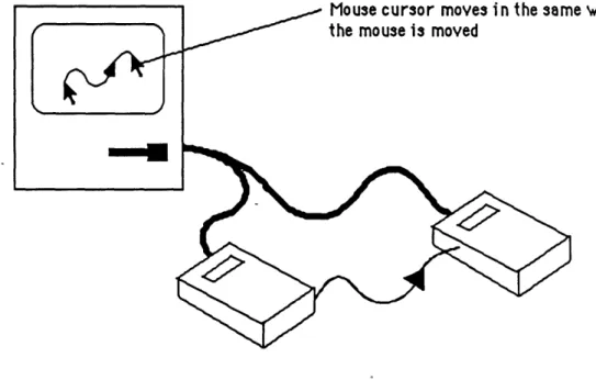
3.2.1 The mouse 50

3.2.2 The desktop 51

3.2.3 The Macintosh environment 53

3.3 The graphic scheduling environment 62

3.3.1 O.S.A. scheduling organization 62

Page 4. FUTURE DEVELOPMENTS AND APPLICATIONS

4.1 Support Algorithms 81

4.2 Schedule drawing-board 82

4.3 Other applications, Scheduling activities of non-Air Transport operations 83

5. CONCLUSION

5.1 On the insertion heuristic 86

5.2 On the graphics interface 86

5.3 On the future 87

6. APPENDIX

6.1 Sample input and output from the insertion algorithm 89

6.1.1 Aircraft data 89

6.1.2 Station data 90

6.1.3 Request data 90

6.1.4 Resulting mission assignment 91

6.2 Effect of different pool sizes in the algorithm 96

LIST OF FIGURES

Figure Page

2.1 Extract of a typical schedule 14

2.2 Simple insertion mechanism 14

2.3 The insertion algorithm as a scheduling tool 16

2.4 Selection of best insertions 19

2.5 Mission list 20

2.6 Data structure of schedules 20

2.7 Current data structure - 21

2.8 Sequential insertion (1) 22

2.9 Sequential insertion (2) 22

2.10 Non-sequential insertion (1) 23

2.11 Non-sequential insertion (2) 23

2.12 Algorithm speed, fixed fleet & variable number of requests 25

2.13 Algorithm speed, fixed number of requests & variable fleet 25

2.14 Mission list with initial requirements 30

2.15 Mission with time wasted at a station 31

2.16 Efficient schedule 32

2.17 Infeasible insertion 32

2.18 Beginning of mission list 33

2.19 Insertion into the schedule 34

2.20 Handling of intermediate stops 37

2.21 Typical activity at a station 38

2.22 Handling of station activity in the M.A.C. system 38

2.23 Process to modify the schedule when an insertion is not feasible 42

Figure

3.1 Relationship between mouse and cursor movements 51

3.2 A typical desktop display with three windows, one folder and

one closed document 52

3.3 The Apple Macintosh desktop 54

3.4 Selection of a command from the menu bar 55

3.5 A typical Macintosh window 55

3.6 Relationship between the "elevator" position and the visible area of a document 56

3.7 Typical event driven system 58

3.8 Graphic object manipulation cycle 61

3.9 Graphic interface organization 62

3.10 O.S.A. scheduling organization 64

3.11 Physical set-up of the new scheduling organization 65

3.12 A.I.S.E.desktop display 66

3.13 The mission display window 67

3.14 Image of the "flight" object 67

3.15 Moving a flight object over the display 68

3.16 Schedule information window 71

3.17 Mission information window 71

3.18 Flight information window 72

3.19 Mission display with cut-off time 73

3.20 The station display window 75

3.21 Organization of flights in the station display 75

3.22 Arriving flight graphic object 76

3.23 Departing flight graphic object 76

3.24 Moving a flight on the station display 77

3.25 Station information window 78

3.26 Dialog window in the mission display 80

1 GENERAL PRESENTATION.

1.1 Background.

Two years ago, the U.S. Air Force Military Airlift Command (M.A.C.) started a major overhaul program to improve its Command and control procedures (C2 upgrade) [ref. 15]. M.I.T's Flight Transportation Laboratory was selected as part of a task force to investigate new ways to support M.A.C. scheduling activities.

The basic recommendations made after one year of research were [ref. 9, 16]: . avoid large -scale optimization algorithms,

- build scheduling graphic workstations to help human schedulers, and

- support parts of the scheduling activity with heuristic algorithms.

Based on these recommendations, M.A.C. asked the Flight Transportation Laboratory to put together a small test scheduling system for the Operational Support Airlift (O.S.A.) which is a small subset of the Airlift Command itself.

This thesis describes A.I.S.E. (Advanced Interactive Scheduling Environment), a scheduling tool which is based on the test system delivered to O.S.A.. The system consists of both a

heuristic support algorithm that automatizes some aspects of the scheduler activities and an extensive graphic interface that can be viewed as a sophisticated electronic drawing board and spreadsheet, entirely devoted to the scheduling task.

This chapter will review the main ideas that lead to Flight Transportation Laboratory's recommendations to the Air Force. In order to set up the environment A.I.S.E. is designed to

work in, the chapter will then briefly describe O.S.A. operations as well as describe the type of problem that must be solved by the support algorithm.

Chapter 2 describes the support "insertion heuristic" that was adapted from the "dial-a-ride" environment. The modifications needed to adapt this heuristic to O.S.A.'s operational environment are extensively studied.

Chapter 3 presents the graphics interactive environment that is proposed to the scheduler and shows how it is linked to the support heuristic. It also reviews special programming considerations that are needed to implement such a system.

Finally, the last chapter discusses possible directions for future implementations of interactive scheduling tools.

1.2. Strategy for scheduling systems.

During the past two decades, most of the efforts made to solve practical scheduling problems resulted in large-scale optimization algorithms running on large mainframe computers [ref. 13, 14]. This approach became dominant because most available computers during that time were essentially number processing machines with very few interactive capabilities. Scheduling was also considered as an activity. quantitative enough to be entirely solveable by pure mathematical techniques.

Overall, the results have been mixed [ref. 3]. The mathematical optimization approach was discovered to have the following drawbacks:

. the size of problems quickly became enormous and required extensive computation time, . the assumptions or simplifications needed to integrate real-life scheduling problems into

the appropriate mathematical framework lead very often to worthless solutions, and - the underlying instability of optimal solutions was unacceptable for real-life operations. For these reasons, large-scale models were found to be appropriate for schedule "planning" but not adapted to practical, every-day scheduling. In their analysis of Aircraft Scheduling [ref. 3],

Etschmaier and Mathaisel conclude:

It was thought for quite some time that scheduling airlines was relatively easy and could

be carried out by a large linear model [...]. Although many closed form endeavors were

begun, none of them were ever completed, but it was hoped that eventually the size and efficiency of computers could catch up and permit some sort of closed form [of the

scheduling problem] to be solved.

The consensus today is that the problem of aircraft scheduling is unsolvable, at least by quantitative techniques.

In the last three years, because computers have become more used as general processors of not only numbers but also text and pictures, researchers have begun to think differently about

the scheduling process. After all, some aspects of manual scheduling such as the types of charts used, appeared to be efficient ways to handle information. Humans were also found to be quite efficient at certain kinds of processing. Finally, the recent arrival of a new generation of graphic oriented microcomputers lead us to investigate a very different approach to solve the scheduling problem. Rather than use a machine to produce an excessively optimal schedule, why not use it to replicate electronically the "paper" environment of schedulers; let them create the schedule, and have the computer check for errors and violations of constraints, manage all the data and display graphically appropriate information when needed.

A first experimental prototype was built and successfully tested by Flight Transportation

Laboratory [ref. 1]. It quickly demonstrated that such an approach took advantage of the processing power of human schedulers. It also showed that some parts of the scheduling activity were indeed quite quantitative and could certainly be handled by heuristic support

algorithms that would produce reasonably good and stable answers to the scheduler.

These ideas resulted in our proposal for a hybrid scheduling environment that would exploit the processing capabilities of both the computer and the human scheduler.

1.3 O.S.A. scheduling problem.

The Operational Support Airlift, a division of the Military Airlift Command, has responsibility for the rapid delivery of Air Force personnel and small cargo to any point whithin the continental United States. O.S.A. uses a fleet of 60 to 80 small business airplanes and satisfies about 200 out of 300 daily requests for transportation. At this time, rejected requests are either accomodated later or simply dropped.

Its activity cycle can be viewed as follows:

1) The requests (see 2.1.1) are filed from 0 to 15 days in advance.

2) A first schedule plan is prepared two days in advance.

3) The schedule is fixed one day in advance.

4) Subsequently, last minute requests can be handled only if their insertion does not modify the schedule.

5) On the day of service, the schedule is monitored constantly.

A.I.S.E. completes these requirements in the following way:

. Step 1 is handled by a data base manager that maintains the list of requests.

. Steps 2 and 3 are executed by both the support algorithm that proposes an initial schedule, and the scheduler who alters it with the graphic schedule. editor in order to account for non-quantifiable constraints.

- The decision support algorithm will also suggest good ways to insert last minute requests into the schedule (step 4); again the solution can be modified by the scheduler.

. Finally, schedule monitoring (step 5) is handled by graphic tools with one exception: after airplanes failures, the decision support algorithm is used to reschedule requests.

The relatively small size of this system made it ideal for a test demonstration that has been implemented on Apple Macintosh microcomputers.

2 THE SCHEDULING HEURISTIC.

2.1 Presentation.

The heuristic selected for the M.A.C. scheduling system is an "Insertion" algorithm initially developped by Dr. J. J. Jaw in order to solve the "Dial-a-Ride" problem. Many similar heuristic algorithms have been developed over the years to solve the Travelling Salesman and the Dial-a-Ride problem [ref. 6, 10, 17] but they usually consider a single pick-up or delivery point. Jaw's heuristic was chosen because it allows multiple pick-up and delivery points and this characteristics made it more appropriate for O.S.A.'s operational environment. In his thesis [ref. 8], Dr. Jaw extensively presents the properties of this algorithm as well as its behavior under various scenarios. We will review here the most fundamental aspects of the heuristic: how it tries to produce an economically good answer and the computational efficiency of the algorithm. We will then investigate the modifications and extensions to this algorithm that are required by the Military Airlift Command specialized operations. Some of these modifications have already been implemented and tested.

2.2 The Insertion Algorithm,

2.2.1 Some definitions,

Let us first review definitions of terms which will appear often in this thesis.

2.2.1.1 Fleet. stations and requests.

The Fleet represents the resources available to the scheduler. It consists of different vehicles each with its own physical characteristics (speed, capacity) as well as economical characteristics (operating costs...).

Vehicles with similar characteristics are said to be of the same type.

The Stations are the different Cities, Airports, warehouses etc..., the vehicles must serve. Their geographical locations define some of the problem constraints such as interstation distances. Other constraints will be defined by more general characteristics of these stations such as curfews, fuel availability, length of runways etc...

Last, the Requests are demands for transportation of cargo, passengers etc... between two stations. They mainly specify the volume to be carried and in our case, the earliest time at which the load will be available as well as the latest time before which it must be delivered. Thus, there is a "time window" constraint associated with each request.

2.2.1.2 Missions and Events.

For each vehicle, a Mission is a sequence of events occuring sequentially at specific times during the scheduling period. These events will usually be of three types:

- Pick-up a specific load at a given station. - Deliver a specific load at a given station.

- Go from one station to another. (In the air transport environment, this will be a flight.)

2.2.1.3 Schedule.

A Schedule consists of a series of missions which are individually assigned to specific

vehicles from the fleet. An extract of a typical schedule is shown in figure 2.1.

2.2.2 Purpose of the Insertion Algorithm.

As its name indicates, the purpose of this algorithm is to insert a specific "request" for transportation into an already established schedule (see figure 2.2). If the request can be

S SCHEDULE MISSION #1 (vehicle 1) MISSION #2 (vehicle 2) mISS (e

Pickup 3 passengers Relocate from CCC Picku in lAR, at 8:30 to LLL, leave @ 6:00 in M Fly from AR to leaving at 8:45 BBB Pickup in ILL, passenger 8:15 4 I' -*f passengers 10:15 4 kup 5 BBB at passengers 11:00 S.,

I

FI

/1

Figure 2.1: Extract of a typical schedule

HEQUEST Transport 5 passengers from ARA to BBB Unfe REQUEST denied

Figure 2.2: Simple insertion mechanism

Deliver in BBB,

inserted in many different ways, some criterion will be used to select the insertion to be retained.

The use of the algorithm can be generalized:

- if the initial schedule is "empty" (no request has been served yet), the sequential insertion of multiple requests will be equivalent to the creation of a new schedule. This turns the heuristic into a complete scheduling algorithm (see figure 2.3.).

. if the schedule is not empty, the algorithm will simply try to insert with minimum disruptions; it will only modify the existing schedule.

In general, the algorithm will be used in a three-step process:

1) Accumulate a certain number of requests and create an initial schedule to satisfy them as

much as possible (scheduling function).

2) Insert last minute requests into this schedule (insertion function).

3) Revise parts of the schedule to accomodate last minute requests of high priority which

cannot be inserted otherwise (mixture of both functions).

2.2.3 The selection criterion,

As we mentioned in the last section, when a request can be satisfied in many different ways a selection must be made. In the current implementation of the heuristic, the selection criterion retained is minimum incremental travel time. Among various insertions, the selected candidate will be the one that increases the duration of a mission by the

le=I

2.2.4 The insertion procedure,

2.2.4.1 Insertion of single last minute requests,

AIRFIELDS BTV 44.28 73.09 BED 42.28 71.17 JFK 40.38 73.47 ATL 33.39 84.26 #7 *****************************************

TYPE = C12 / STATION = BTV / TIME WHEN

CAPACITY = 5 / SPEED(KNTS) 420

ITINERARY :

AVAILABLE = 04:00

BTV ATL JFK BTV

SCHEDULED DESIRED

BASE MODE TIME TIME

BTV ATL JFK BTV 04:00 06:49 09:13 23:00

PAX ONBOARD REMAIN. ON/OFF LOAD CAP.

06:00 10:00

S**********************************************************

Figure 2.3: The insertion algorithm as a scheduling tool

S , .c0 - u E w o0 0 00 -1 m C21 DCA 5 06:00 23:00 420 C12 BTV 5 04:00 23:00 420 T39 BED 6 07:00 23:00 420 T39 LAX 6 05:00 23:00 420 0, .0 E a) 0) 40 0 Cn C .0 cn 0, SF0 STL 04:00 09:00 3 1 1 LAX STL 07:00 12:00 7 2 1 SF0 JFK 12:30 23:00 5 1 1 STL MIA 11:00 19:00 2 1 2 DCA ATL 14:00 18:00 3 1 2 MISSIONS **** AIRCRAFT

Insertion Algorith~m

Phase 1:

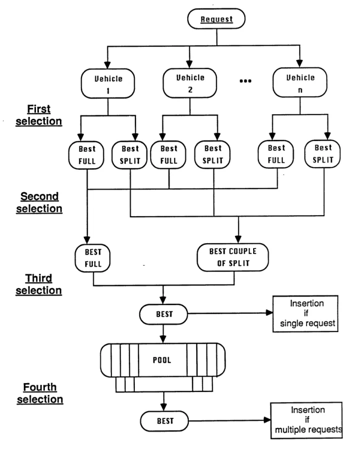
For each vehicle in the fleet, establish all possible ways the request can be inserted into the current schedule.

At this point, account only for the time constraints. Compare all possible solutions and select:

. the best one that can carry the full load

. the best one that can only carry part of the load (due to limitations on the remaining space available).

Phase 2:

. For the "full load" solutions, compare the best answers among all vehicles and select the best one.

- For the "split load" solutions, look at every possible combination of two best answers among all vehicles and select thebest pair that can accomodate the full load. (Iq the current implementation a pair's travel time is the sum of the travel times with each vehicle.)

Phase 3:

Compare the "full load" and "split load" solutions and select the best one. If both solutions add the same incremental time, choose the "full load" answer. If no feasible insertion can be found at the end of phase 2, the request is rejected.

2.2.4.2 Sequential insertion of multiple requests (initial scheduling).

1) The initial processing of each request is executed with the 3 phase process described

above.

2) The best solution is then inserted into a "pool" of n answers which already contains the best solutions corresponding to n- 1 previous requests from the request list.

have different priorities, higher priorities will always be chosen first.

4) At this point, the remaining n-1 solutions will be re-calculated, taking into account the new insertion, and a new request will be pulled from the list in order to keep the pool always full.

First

selection

Second

selection

Third

selection

Fourth

selection

2.2.5 Data structure associated with the schedule,

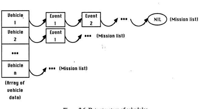
A very flexible internal data structure has been chosen to represent each vehicle's mission.

It is based on the events described in 2.1.2.

Considering that each mission is a succession of events during the scheduling period, it is represented as a linked list of event data records:

Figure 2.5: Mission list

Adding in the vehicle data itself, the global schedule is represented in computer memory as

follows: Vehicle Uehicle 2 fee Uehicle n (Wrrag of uehicle data) 2 _{fee NIL} (Mission list) Euent

ese (Mission list)

gs (Mission list)

Fieure 2.6: Data structure of schedules

Figure 2.7 gives a full description of the structure with details of the content of the event record.

Vehicle type Vehicle type

Capacity Cpct

Ptr. to mission list Ptr. to mission list

Ptr. to previous item Ptr. to other euent of the request Station of event (1) Type of request (2) Uolume of request Priority of request Split indicator (3) Time constraint (4) Time of occurence (5) Remaining capacity (6) Ptr. to next item Ptr. to preuious item Ptr. to other euent of the request Station of euent Type of request Uolume of request Priority of request Split indicator' Time constraint Time of occurence Remaining capacity Ptr. to next item

(1): R station indeH is used rather than the name (2): P for pickup, D for delivery (3): 1 if load is not splitable

2 if it is

(4): Earliest pickup time or Latest delivery time (5): Time at which the event

starts

(6): Capacity remaining on board once the event has been

eecuted (decreases if Pick-up, increases if Delivery)

Fieure 2.7: Current data structure

Ptr. to preuious item Ptr. to other euent of the reque

f

2.2.6 General comments,

In light of the above descriptions, a few comments can now be made.

1) The handling of split loads was not part of the original "Dial a ride" insertion algorithm.

2) Even though three types of events were described earlier, only two -pick up and delivery- will appear in a mission list since it is assumed that a vehicle has to move between two successive events which occur at two different stations.

3) This algorithm is a "forward insertion" heuristic: it will always insert a new event after

an old one. For this reason, only four types of insertions will be possible for a request, (remember that an inserted request will consist of two events, a pick up and a delivery): - Sequential insertion at end of schedule:

Pickup 0 eliuery

Event N IL

(old link)

Figure 2.8: Sequential insertion (1)

- Sequential insertion between two events from the mission list:

Pickup Deliuery

Euent Euent

(old link) Old list

Figure 2.9: Sequential insertion (2)

Pickup Delivery

Euent Euent Event NIL

(old link) (old link)

Figure 2. 10: Non-sequential insertion (1)

. Non-sequential insertion anywhere in the schedule:

Pickup Deliuery

Euent E ent Event EDent

(old link) (old link) Odls

Figure 2.11: Non-sequential insertion (2)

. Practically, when the heuristic tries to insert a new request into a mission list, it will skip over the events which occur before the earliest time at which the load will be available. Then, in order to find a feasible insertion, the algorithm will try each of the four types just described, using the remaining events of the mission list.

The last three types of insertion may require the algorithm to push forward (i.e. later) in time some already scheduled events. For instance, let us suppose that a vehicle went from station AAA to BBB in its original mission; all pick-up's and deliveries occuring in BBB and after must be delayed to a later time if we want the vehicle to go from AAA to CCC and only then to BBB. The incremental trip time will be equal to the trip time from AAA to CCC plus the trip time from CCC to BBB minus the old trip time from AAA to BBB. If this process does not violate any of the latest delivery constraints, the insertion will be considered as valid.

This behavior triggered the name "forward insertion" since events can be inserted only after

2.2.7 Performance of the algorithm, 2.2.7.1 Size of the pool.

The pool (see 2.2.4.2) is the area where a certain number of feasible insertions are kept for comparison before the fourth selection process (Figure 2.4). With a larger number of slots in the pool more insertions can be compared and the resulting schedule should be better. Different sizes, ranging from 1 to 5, have been experimented with, using various test cases. The elements retained to evaluate the schedule produced in each case were the number of passenger-miles flown, the average system load-factor and the total travel time required by the schedule. The results are shown in Appendix 6.2.

As Jaw showed in ref. 8, increasing the pool size does not produce any specific improvement. In our example from the appendix, we can even observe a deterioration of the schedule with larger sizes. However, in other cases which were tested, pool sizes of 1 and 2 gave obviouslysbad schedules with many rejected requests. Improvements came only with a size of 3. Overall, there is-no systematic trend and the "goodness" of the solution seems to depend only on the order in which requests are presented for insertion.

After some experiments it was decided that a pool size of 5 would be a possible compromise between producing a good schedule and not increasing substantially execution time. For the time being, results produced by the insertion heuristic are at least as good or better than those produced by human schedulers. However, further research is needed; a better optimization objective-function must be defined, and the procedure to select best insertions must be improved.

2.2.7.2 Execution time.

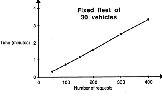
The timings shown on figures 2.12 and 2.13 were derived, using an Apple Macintosh computer. The time is measured from the beginning of the insertion process to its end. Set up time is not counted, neither is the time it takes to produce the results report.

Surprisingly, when one parameter (fleet size or number of requests) is fixed, calculation times seem to increase linearly with the other parameter. This is not true. In fact, the

problem solved is so small that its real calculation time is hidden by a substantial computer operating-system overhead. Jaw has shown [ref. 8] that computation times needed by the insertion heuristic are proportional to V*(R/V)3 with V vehicles and R requests.

Time (minutes)

Fixed fleet

100 200 300

Number of requests

Fieure 2.12: Algorithm speed. fixed fleet & variable number of requests

Time (minutes)

Fixed number of

requests

(200)

Figure 2,13: Algorithm speed. fixed number of requests & variable fleet

of

30 vehicles

400

30 40 50 60 70 80 90 100 Number of vehicles

2.3 Modifications and extensions over the original insertion

algorithm for the dial-a-ride problem,

Most of the extensions which will be discussed here, were needed in order to satisfy the Military Airlift Command operational requirements. Even though some of them may be very specific to M.A.C. type of activity, most extensions would be needed in a general purpose scheduling system.

When discussing the graphics aspect of A.I.S.E., other requirements will be studied which do not involve the insertion heuristic.

Let us first review the M.A.C. requirements which necessitate modifications or extensions to the algorithm. Their actual implementation will be discussed afterwards.

2.3.1 Description of operational requirements. 2.3.1.1 Duration of events.

The current implementation of the algorithm assumes that each event is instantaneous. For instance, if a pick-up occurs at 10:00 the vehicle can leave the station at the same time. This assumption is obviously unrealistic and must be modified.

2.3.1.2 Return to base. return to predefined station.

A vehicle located at a station at the beginning of the scheduling period may be forced to

return to that original base no later than a specified time.

A natural extension of this assumption is to be able to force the vehicle to return to any

specified station.

2.3.1.3 Maximum Crew duty.

Each mission is served by one crew and there can be some constraints on how long a crew can remain operational during a scheduling period. This limits the duration of all missions.

M.A.C crews have a maximum duty time of 16 hours per day in peace time; their duty day

2.3.1.4 Operational range of vehicles,

There usually are some restrictions on how far a vehicle can go without refueling. This means mainly that certain stations cannot be linked by a direct, non-stop service.

2.3.1.5 Minimum time on ground.

In the case of passenger transportation, boarding and disembarking events have a very short duration and an efficient schedule could become very "tight" and quite sensitive to unexpected events such as weather delays, minor breakdowns etc... In order to introduce some slack in its operations and give some margins for small delays, M.A.C. requires a minimum of one hour on the ground at any station.

2.3.1.6 Stations restrictions.

There may be some constraints at specific stations, which should be taken into account when the schedule is established.

The most important ones will be:

- curfews : vehicles may not leave or arrive at a station during a certain period of time. . maximum number of vehicles at a station at any given time: a station may have a limited

number of parking slots.

. maximum handling capacity : there may be enough parking space but not enough equipment to unload more than a certain number of vehicles at the same time.

- runway length: in the case of airplanes there may be some physical constraints limiting the access to certain stations.

2.3.1.7 Force a vehicle to stay at a station.

Again, in the case of passenger transportation, many requests will really consist of two requests:

- Pick up somebody at a station and take him to another station (for a meeting). - Take him back to the first station (after the meeting).

Very often, however, these requests are left open-ended: the return travel earliest time will depend on the meeting itself. Under these circumstances M.A.C. ensures the availability

of a vehicle for its V.I.P's by keeping it ready on the ground as long as necessary. During that time the vehicle cannot be used to satisfy any other request.

2.3.1.8 Force a vehicle to provide a non-stop service.

Even though the service will be provided within the desired time constraints, some individuals might require service in which they are transported from one station to another without many stops in between to pick up or unload other passengers.

2.3.1.9 Keep the departure times unchanged.

When the insertion process has reached the second stage where last minute requests are handled, the algorithm might find a feasible solution by pushing forward in time some of the services provided by a vehicle.

Unfortunately, if a scheduler has already transmitted the schedule to the individuals who placed the requests, it might be desireable not to touch the departure times at all in order to avoid too many late changes.

2.3.1.10 Force an infeasible request to be inserted and/or replace other requests of lower

priority.

Once an initial schedule has been established, all subsequent requests will be inserted only on top of it. Prior requests already inserted will never be removed. It is possible, therefore, that at a certain point the schedule becomes so dense that no further request can be served, whatever its priority.

If a last minute request of extreme urgency is presented to the scheduler, it may not be acceptable to have the system simply reject tharrequest if its insertion into the old schedule is infeasible. A way should be provided to allow this request to replace any other request of

lower priority or, if this is not enough, to be inserted into the schedule before any request

of same priority.

2.3.1.11 Fix schedule up to a cut-off time and reschedule afterwards.

If a long series of last minute requests is presented to a scheduler who has already released the schedule to operations, he (she) might want to modify it only after a certain time in order

to minimize short term disruptions and changes.

2.3.1.12 Reschedule missions following a vehicle failure.

This is certainly one of the most difficult task for the scheduler. For this reason it has usually been handled in the most straightforward way: leave the other missions untouched, relocate a spare vehicle to the station were the failure occurred and resume the mission with a substantial delay...

However, an optimized rescheduling will often decrease the negative impact of vehicle failures by re-routing more than one vehicle and spread the effect of these failures over more missions. Such a capability should be added to our system.

Having reviewed these requirements, let us now return to the algorithm and see how it can be modified or extended to account for them.

2.3.2 Addressing the operational requirements. 2.3.2.1 Duration of events,

A very simple modification was made:

1) Add an event duration field to each event record of the mission list.

2) Modify all the time and schedule calculations in order to account for this term.

2.3.2.2 Return to base.

Here, rather than altering the insertion algorithm, we decided to make use of "dummy events". These events consist of pick-ups and deliveries of "null" loads (0 passenger, 0 pallet of cargo...) which are inserted into mission lists in order to force vehicles to be at specific stations at specific times.

Suppose that our vehicle must return to its base no later than time T. The schedule is first initialized with a dummy delivery that makes the vehicle start from the morning base. The time at which this delivery occurs will be the beginning of the scheduling period (when our

vehicle becomes available). Following this initial delivery, the algorithm inserts a dummy pick-up followed by another dummy delivery. All three events occur at the same station.

a) The second dummy delivery has a latest delivery time set equal to T in order to ensure that the vehicle returns no later than T.

The event duration of this delivery is set to infinity to avoid the insertion of requests after the return to the base.

b) The dumny pick-up has an earliest available time set to T and a duration equal to zero.

This dummy pick-up is necessary to keep the pick-ups and deliveries matched. This requirement is not crucial in the current algorithm, but may become so in future extensions. Another reason for including this activity is algorithm efficiency since certain tests of feasibility are done using pick-up events.

Finally, for overall consistency, the time of occurence of both events is set to T.

Figure 2.14 shows how initial requirements will be translated into the initial "empty" schedule. Suppose these requirements were: Vehicle V will be ready in AAA at time T =

07:30 and will have to return no later than T = 23:00. The initial mission list for vehicle V will be:

LDT = 07:30 EPT = 23:00 tim LDT = 23:00 On =00:00 O n =00:00 Dn =c TO =07:30 TO =23:00 TO =23:00 Legend: P = pickup, 0 = delivery ST = station name

EPT =earliest pickup time, LOT = latest delivery time

On = duration of euent

TO = time of occurence for euent

If the vehicle must return to a station different from its base of origin,the station of both dummy events can simply be changed accordingly.

Finally, if the scheduler wants the vehicle to return to a specific station without any time limit, the latest delivery time of the dummy delivery can be set to infinity.

2.3.2.3 Maximum Crew duty,

This constraint can be checked by keeping track of the total mission time for each vehicle. This time includes both moving time as well as time spent at each station.

At the first and last stations of the mission, the time to be considered should be respectively vehicle preparation and "deactivation" time.

When a new insertion is considered, the algorithm should simply add to the current mission time the extra time required and check that the sum remains within the limit. If not, that particular insertion will be dropped from further considerations.

Since each request is served as early as possible, it is possible that a vehicle leaves at the beginning of the schedule period in order to serve an early request or relocate itself to another station where service will be needed. Often, this early move will be followed by an extensive time on the ground in order to wait for the next load to be available for pick-up. For instance, we will have:

ARAA BBB

Leave

empty

Arrive

Stay at

Pickup

Leave

at 6:00 at 7:00/ station

/

(Pickup duration

= 00:30)

Figure 2.15: Mission with time wasted at a station

RAA BBB

Leave empty

-Arrive/ Pickup

/

Leave

at 9:00 at 10:00 at 10:00 at 10:30

(Pickup duration

= 00:30)

Figure 2.16: Efficient schedule

However, if the first leg is pushed forward in time, we have seen that the algorithm has no ability to move it back. The following new insertion will therefore become impossible:

RAN CCC BBB

6:00 6:30 7:30 8:00 9:30 10:00

Figure 2,17: Unfeasible insertion

For this reason, the dummy delivery event simulating the time at which the

vehicle becomes available should -never be moved forward. Rather, when computing the mission duration, the algorithm should assume that the vehicle will leave on it's first trip as late as is compatible with the first latest delivery constraint. When evaluating new possible insertions, the mission time will be increased as described above only if the insertion does not involve the first trip. If it does, the duration will be recalculated not using the time of the first dummy delivery but assuming that the new first request is served as late as possible.

Let us clarify this approach using the previous example. Before evaluating insertions, the beginning of the mission list for our vehicle was:

PI ST = AAA P S=BB

EPT = 06:00 EPT = 10:00

On =

00:00

TO =06:00 TO =10:00

Legend: See figure 2.14

Figure 2,18: Beginning of mission list

This list must be interpreted as:

- The vehicle is available at 6:00 in AAA.

- It will go from AAA to BBB totally empty (relocation). . Finally, it will pick up a load in BBB at 10:00.

According to the principles discussed above, mission length will be calculated by adding the following terms:

- One hour for vehicle preparation.

- One hour to relocate the vehicle from AAA to BBB (this move is assumed to occur as late as possible from 9:00 to 10:00).

- Thirty minutes of ground/loading time in BBB. - Etc...

If no "special treatment" was given to the first leg of the mission, the time calculation would assume that the relocation occurs between 6:00 and 7:00 and add a three hour stay on the ground (entirely wasted) in BBB.

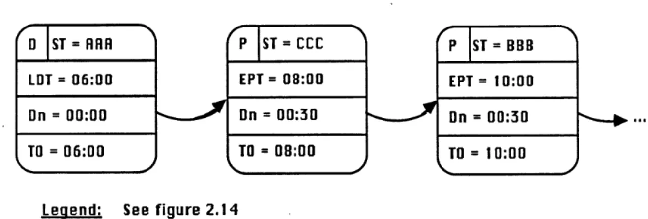
Let us now suppose that part of a new request to be inserted is: Pick up a load in CCC with EPT=8:00 and Dn=O:30.

(Moving times are respectively: one hour from AAA to CCC and one hour from CCC to BBB).

Du ST = AR A AP ST = CCC P ST = BOB

LDT= 06:00 EPT= 08:00 EPT = 10:00

On = 00:00 On = 00:30 On = 00:30

TO = 06:00 TO = 08:00 TO = 10:00

Legend: See figure 2.14

Figure 2.19: Insertion into the schedule

Mission length should now be calculated by adding the following terms: * One hour for vehicle preparation.

- One hour to relocate from AAA to CCC (again assume a departure as late as possible at 7:00 and not 6:00).

. 30 minutes for loading in CCC.

- One hour to go to BBB (from 8:30 to 9:30). . 30 minutes waiting on the ground at BBB.

. 30 minutes to load in BBB.

- Etc...

As one can see, if the minimum ground time requirement is ignored, there are still 30 minutes lost in BBB. One solution could be to move flight AAA to CCC forward by 30 minutes.

Unfortunately, this tactic would not be compatible with the algorithm implicit "policy": serve each request as early as possible. There is, however a definite tradeoff. Experience only will show whether it is better to serve each request as early as possible or implement a "compaction algorithm" which would push events around in order to minimize time wasted on the ground.

At the end of the mission, the same problem will occur only if a "return to base" constraint is implemented. In other cases, the algorithm will schedule events as early as possible

insuring the earliest possible arrival at the last station of the mission.

In the "return to base" case, the problem can be easily fixed by changing the constraint implementation previously described (see 2.3.3). The "earliest pick up time" of the dummy pick up event should be changed to the time at which the vehicle is available at the beginning of the scheduling period.

The algorithm will try to serve this dummy request as early as possible but because of the infinite duration of the delivery all requests will be inserted before it.

With this new set up, we can expect to see the two dummy events separated by other pick up or deliveries. Very likely, the dummy pick up will be the first event served in the morning if the return has to be at the base (since the vehicle is already at the base, it does not cost anything to insert the dummy pick up at this point). In fact, if it appears that any matching of events (one pick up for one delivery) is not crucial, the dummy pick up could be removed.

2.3.2.4 Range of vehicles,

When the insertion of a request necessitates a new movement from one station to another, -the algorithm should check that the distance is less than the maximum range of the concerned vehicle. If the range is not sufficient, however it is not possible to simply reject the insertion.

Suppose for instance that we have: . 3 stations:

BBB

ARAA

range of

vehicle _CCC

0

. one vehicle whose range is not enough to go directly from AAA to CCC.

If the first request is for service between AAA and CCC, the range constraint would force the algorithm in its current state to reject it. AAA to CCC would never be feasible; this is obviously wrong. On the other hand, if the first request is between AAA and BBB and if this trip leaves enough space for the AAA-CCC load, then the service from AAA to CCC will become perfectly feasible with a stop in BBB. The feasibility of "out of range" requests depends on the order in which they appear in the request list.

For a specific request, if the best insertion appears to be infeasible due to range restrictions, the following strategy could be used:

(1)Find an appropriate feasible multi-stop itinerary. - by asking the scheduler, or

- by looking into a data base where possible itineraries could be stored in advance or upon request.

(2) Calculate the "cost " of providing the service with that itinerary.

(3) Compare it to the best entirely feasible insertion (if any).

(4) Take the cheapest one.

The insertion of a multi-stop itinerary will be done with two dummy events inserted at the intermediate station:

. a dummy delivery of the load, with an event duration of 0 minutes followed by:

vehicle.

For a load to be carried from AAA to CCC with an intermediate stop in BBB, the mission list will be:

E

Es

STB

=ccC

EPT = ... LOT = oo EPT =morning EPT=..

On = ...e On = 00:00 Dn =refueling On=..

TO = TO =arriual TO =arriual TO

Legend: See figure 2.14

Figure 2.20: Handling of intermediate stops

The latest delivery time and earliest pick up time of the dummy events are set respectively to infinity and to the start of the scheduling period. They should not interfere with the other events.

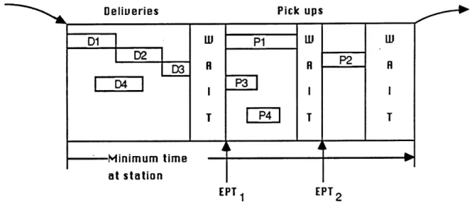
2.3.2.5 Minimum time at stations,

In every case, the time spent at the station can be divided as follows:

1) Just after the arrival, a first time period is needed to unload. the vehicle.

2) Then there is a waiting period until a first load is available for pick-up.

3) The third period is the loading period that may include other waiting periods if the loads

to be picked-up are not quite ready.

4) A final waiting period will be required only if the minimum time at the station is more than the length of all previous periods.

The duration of the loading and unloading periods will depend on the following factors: . Duration of individual pick up and delivery events.

. Whether these events are parallel ( more than one piece of cargo can be unloaded at the same time) or sequential (if the vehicle has only one door for instance) .

. Earliest pick up times.

All these elements are summarized in the following figure.

Deliveries

-Minimum time at station

EPT_{1 EPT 2}

Figure 2.21: Typical activity at a station

In the case of our system, only passengers will be transported. Consequently, the loading and unloading times will always be very short and altogether less than M.A.C. required minimum time at a station.

Also, because passengers do not like to wait inside a vehicle that is not moving, we suggest handling the constraint as follows:

U N _L L W R I T 0

0

_R

Figure 2.22: Handling of station activity in the M.A.C. system Pick ups

1) Assume that each pick up or delivery event has a duration of say 15

minutes and that they all occur in parallel. 2) Thus:

- set the start time of delivery events to the landing time, their duration to 15 minutes. - set the start time of pick up events to (Landing Time + Minimum Time At Station -15 Minutes) and their duration to 15 minutes.

2.3.2.6 Station Restrictions,

Most of the restrictions listed in 2.3.1.6 can be handled with a simple check by the algorithm when a new insertion is being evaluated.

" If a station has any constraint on the vehicle types, insertions will be tried only on

appropriate types.

- If any curfew exists, insertions with inappropriate pick up or delivery times will be rejected.

- etc...

The limit on loading/unloading equipment will require a different processing. It will mainly affect the length of time spent at a station since the vehicle will have to wait for the equipment to be available.

2.3.2.7 Force a vehicle to stay at a station.

This constraint can be handled by setting the delivery duration to infinity. The system will not schedule any event after that delivery and the vehicle will stay at the station indefinitely. Unfortunately, this setting would also lead to an inconsistent state of the system since ultimately the vehicle will return to another station. If that station is known in advance, the "return to station" dummy events should be added at the end of the mission list.

In the following chapter we will see how the system should interpret the mission list to derive the schedule as well as the list of stations where overnight stays will occur.

2.3.2.8 Force a vehicle to provide a non-stop service.

The scheduler will have the ability to 'attach" the non-stop constraint to a request. If he does, the algorithm will:

1) Evaluate only the non-stop insertions, if any.

2) Set the earliest pick up time and latest delivery time such that

LDT -EP = flight time

This choice will insure that no other request be served through an intermediate stop which would require some extra time over the original non-stop service time.

2.3.2.9 Keep the departure times unchanged,

This constraint will be handled by the algorithm when checking the feasibility of new insertions. If the insertion requires to move forward in time any event already scheduled, it will be eliminated and considered infeasible.

If the scheduler wants such a constraint to be active,. it can be expected that feasible insertions will become much more difficult to find.

2.3.2.10 Force an infeasible request to be inserted and/or replace other requests of lower

priority.

This requirement is one of the most difficult to handle because it requires a change to the initial schedule rather than an addition to it.

If a last minute request of priority p cannot be inserted into the current schedule, the scheduler has two ways to deal with it:

1) Consider that it was presented to the schedule after all previous p requests. In that case, all requests of lower priority (p+l,p+2...) should be removed from the schedule , and the insertion should be retried. If it remains infeasible, the scheduler can justify the rejection of the request by its lateness with respect to other requests of same priority.

2) Consider that it was presented to the schedule before all previous priority p requests. Here, all requests of priority p and less should be removed before the insertion is retried. If it is rejected once more, the justification will simply be that there are already too many requests of higher priority being served. In short, the priority is not high enough.

Let us now investigate how requests should be removed from the schedule.

If the schedule is kept unchanged and the appropriate events (priority p+l,p+2, etc...)

simply removed, the final result will not be very good. During the previous scheduling process, the insertion of these lower priority events requires pushing forward in time some of the higher priority events already inserted. If the low priority events are removed, the remaining events will still be "pushed forward" and as we have seen, the algorithm will not

be able to move them back in time.

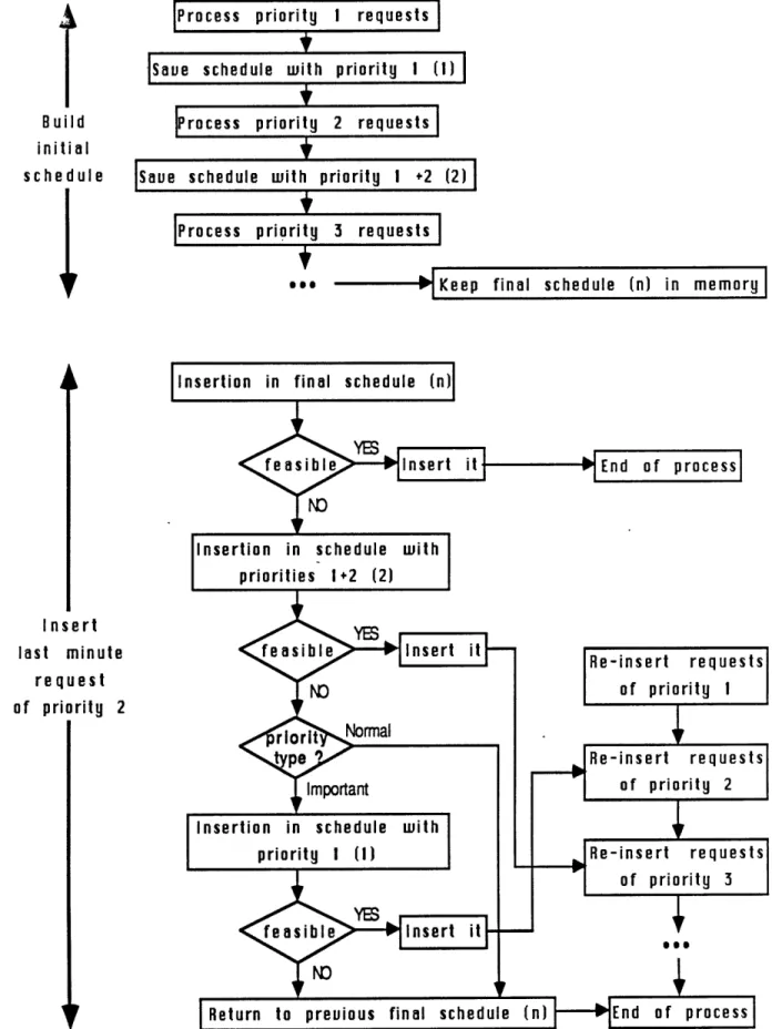
It is therefore more appropriate to "remove" lower priority events by returning to the schedule obtained before these events were inserted. The algorithm should save the schedule it has produced in a file, each time a request with a new (lower) priority is about to be inserted.

The new process is described in figure 2.23.

Let us now look at two problems associated with this process.

1) Computation time and number of changes,

As shown in figure 2.23 each time a last minute request needs to be inserted, all lower priority requests have to be re-inserted afterwards. The insertion will therefore become quite long if the request is of high priority; basically the whole schedule would have to be recalculated. Moreover, even though the new request will be served by one or two vehicles at most, the new insertion could affect the missions of other vehicles as well.

If execution speed is critical or if it is important to keep the schedule intact as much as possible, the previous strategy could-be changed as follows:

I

4

Saue schedule with

Process priority

SSaue

schedule with p

IProcess priority

Figure 2.23: Process to modify the schedule when an insertion is not feasible

I requests priority I (I)

2 requst

riority 1 2 2

3 requests

. keep the new schedule only for the affected vehicles, - reinstall the previous final schedule for all other vehicles,

. re-insert the requests displaced by the new insertion only. Modify all intermediate schedules as needed.

Experiments only will show if a schedule produced in this manner is much worse than one obtained by rescheduling all lower priority requests.

Depending on the results there may be some tradeoffs involved between keeping the schedule intact and making it as efficient as possible.

2) Feasible last minute requests,

Let us suppose that before an infeasible priority 2 request was presented to the scheduler, two other priority 1 last .minute requests had been successfully inserted. Since these 2 requests were not part of the original list, they will not appear in any of the intermediate schedules saved in data files. If the new process described in figure 2.23 is used, these requests will not be served any more since the system restarts from one of the intermediate schedules. To avoid this undesireable effect, the following steps should be added to the process:

a) If a last minute request is successfully inserted, add it to a stack. (each priority should have its own stack).

b) If a rejected last minute request must be inserted, rebuild the schedule by inserting at

each priority level

- the requests from the appropriate stack if it is not empty, - the rejected request when its priority has been reached.

c) Empty all the stacks and add their requests to the main request list.

the scheduler the capability to serve an infeasible request by adding a spare vehicle to the active fleet.

2.3.2.11 Fix schedule up to a cutoff time and reschedule afterwards.

The major difficulty with this feature will be the selection of events that should be kept or even fixed in the schedule once the cutoff time has been selected.

Practically, around that time a typical vehicle will either: . be at a station, totally empty [case I], or

- be at a station, but with a load in "transit" [case II], or

- be moving from one station to the next with a load on board [caseII].

Case I is the most simple to handle. All requests that were served prior to cutoff time are left unchanged into the old schedule; the others are put back into the request list. A new schedule is then initialized in which the vehicle is simply available at cutoff time at the

station where it stopped.

Case II requires the scheduler to make some decisions. As in case I, all the requests entirely served (pick-up and delivery) before cutoff time will be kept in the old schedule; all those for which the pick-up will occur after cutoff time are put back into the request list. The requests in transit (pick up has been done but not delivery) cannot be handled as easily: two strategies are possible.

- Cancel the pick-up event of the transit request and put the request back into the request list. This makes the old schedule less efficient, but keeps the insertion process simple and free to build the new schedule optimally.

- Keep the pick up event and force the delivery to occur in the new schedule. The old schedule remains untouched but the new one will not be as efficient as possible (within the limits of the algorithm) since it has to deliver the requests in transit.

If the second strategy is selected, the new schedule will have to be prepared with all necessary events appropriately placed:

- the dummy delivery at the beginning for the availability information,

. the deliveries of requests in transit as early as possible (since the algorithm can only push them forward in time),

- the dummy pick-up and delivery at the end, if any "return to station" constraint is active.

Again if it is important to have a match between pickups and deliveries, the deliveries from requests in transit could be balanced with dummy pickups of the appropriate load at the new station of origin.

Case III will be turned into case I or II as soon as a station is selected as the origin of the new schedule. This station can either be the one the vehicle is coming from or the one it is going to . If the system has to be automatic , it could select the station

. which is after cutoff time (in order to keep the old schedule as untouched as possible), or

- which has the least number of requests in transit (in order to allow for more optimality), or

- which is closest to cutoff time.

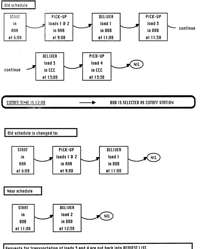
It may be appropriate, however, to leave the choice to the scheduler. Figure 2.24 summarizes the handling of cutoff time by an example.

Old schedule

STRT |1

continue

continue

CUTOFF TIHE IS 12:00 - BBB IS SELECTED RS CUTOFF STATION

Old schedule is changed to:

STR RT PICK-UP DEllUER

i n loads 1 D' 2 load 1

RRR in RRR in BBB

at 6:00 at 9:00 at 11:00

Neu schedule

STaRT DElb TER

in load 2

BBB in000

at I11:00 at 12:30

Requests for transportation of loads 3 and 4 are put back into REQUEST LIST.

2.3.2.12 Reschedule missions following a vehicle failure.

This last extension to the insertion algorithm can be handled in two different ways.

1) Re-insertion of affected requests,

With this technique, the rescheduling process is automatic. First, the scheduler makes all spare vehicles available to the system. Then, the insertion algorithm is used to reinsert all the requests affected by the failure:

. requests not yet served (pick-up not done); the request specifications remain unchanged. - requests not yet delivered; the specifications are changed to reflect the fact that these

requests must now be picked-up at the station where the failure occured.

The advantage of this approach is that it will try to reschedule with minimum incremental time. The solution, however, may not be acceptable to the scheduler if some requests are rejected or if some missions are substantially modified. In order to give the user more control, we suggest also the following heuristic.

2) Manual rescheduling.

Even though we consider this modification as. an extension, it may be more appropriate to view it as another decision support tool which can be used in parallel to the insertion algorithm.

Since a failure is a dynamic event which becomes known only when it occurs, the task of the scheduler is to find out which vehicle are, or will be, available after failure time, and figure out if some of these vehicles can be used to solve the problem.

This process can be decomposed in the following way:

1) Get failure information:

-Current time: CT

-Vehicle type: V

-Estimated repair time: RT

-Station at which failure occured: AAA