Aeroelastic Study of a Multi-Hinged Wing
byTorrey Owen Radcliffe
S. B., Aeronautics and Astronautics Massachusetts Institute of Technology (1997)S. M., Aeronautics and Astronautics Massachusetts Institute of Technology (2002)
Submitted to the Department of Aeronautics and Astronautics in Partial Fulfillment of the Requirements for the Degree of
DOCTOR OF PHILOSOPHY IN AERONAUTICS AND ASTRONAUTICS
at theMASSACHUSETTS INSTITUTE OF TECHNOLOGY
MASSACHUSETTS INSTITUTE
February
2003
OF TECHNOLOGY@ Massachusetts Institute of Technology 2003. All rights reservd
SEP
1 0 2003
Author
LIBRARIES
uepartment of Aerona s and Astronautics October 15, 2002 Certified by Certified by Certified by Accepted by (i Carlos E. S. Cesnik
Visiting Associate Professor of Aeronautics and Astronautics Chair, Thesis Committee
Mark Drela Professor of Aeronautics and Astronautics Member, Thesis Committee
(I
kohn DuguAdjiProfessor Emeritus of Aeronautics and Astronautics Member, Thesis Committee
Edward M. Greitzer H. N. Slater Professor of Aeronautics and Astronautics Chair, Committee on Graduate Students
Aeroelastic Study of a Multi-Hinged Wing
by
Torrey Owen Radcliffe
Submitted to the Department of Aeronautics and Astronautics on October 15, 2002, in partial fulfillment of the
requirements for the degree of
Doctor of Philosphy in Aeronautics and Astronautics
Abstract
Dynamic aeroelastic response of multi-segmented hinged wings is studied theoretically and experimentally in this thesis. For the theoretical study, a method of modeling the aeroelas-tic characterisaeroelas-tics of multi-hinged wings is proposed. The method employs the Runge-Kutta scheme to solve the governing equations of a flexible multibody dynamic system. The Henon method is used to switch between bilinear stiffness states of the wing in bending. Exper-imental wind tunnel tests of one- and five-hinged wings were conducted for better insight into the mechanics of the motion. Correlation between the experimental and theoretical results is presented. The theoretical model is found to capture both the linear and nonlinear aeroelastic behavior of a hinged wing. Adding hinges to a wing is found to significantly alter the speed at which an instability will occur. The stiffness of the hinges is found to play a major role in the determination of flutter speeds with a reduction in hinge stiffness nominally leading to an increase in first bending
/
first torsion instability speeds. However, for low hinge stiffness, hinged wings were also found to have the possibility of a second bending/
first torsion instability at speeds far below the first bending instability. The hinged wing is found to enter into chaotic or limit cycle motion at speeds at, near, or above flutter speeds. The bi-linear nature of a hinge is found to cause a disruption in the coalescence of modes. This limits the energy added to the system while it is in an unstable state. The hinges allow the wing to "fold" under low net loads. The theoretical model can be used for aeroelastic design of future hinged wings for remotely deployable vehicles.Thesis Supervisor: Carlos E. S. Cesnik
Acknowledgments
There are many people who I wish to thank for their help and support which made this possible. First, I would like to thank my advisor, Professor Carlos Cesnik, who introduced me to the field of aeroelasticity. Without his guidance none of this would have been possible. Despite taking a position at a different university, Professor Cesnik was willing to support all of his old students through the finish of their degrees. On top of that, he is able to spot a sentence with a missing comma from a hundred paces.
Professor John Dugundji was always able to offer a bit of helpful advise on structural dynamics, experimental flutter work and thesis preparation. Professor Dugundji was kind enough to take over for much of the advisor duties that Professor Cesnik could not perform from a distance.
Professor Mark Drela was able to provide invaluable support helping to stir the thesis on the proper course. I would also like to mention Professor Karen Wilcox and Tienie van Schoor who were kind enough to read the thesis before the defense despite its numerous spelling errors.
Professor Eugene Covert, Frank Durgin, Richard Perdichizzi, and Jadon Smith were invaluable in their assistance with the wind tunnel experiments. I would like to thank all of the people who worked in TELAC and put up with me taking up all the computer time to run my inefficient code. A special thanks to Dennis Burianek, who taught me the in's and out's of using I4TEXwhich this manuscript was written in.
My room-mates Matthew Congo and Nicole Krumrei have always been there to help me
take my mind off of my work and to read through some of the early drafts of this work. I also need to show my appreciation for all the support and encouragement I relieved from Andrea Green over the years, and the years to come.
A special thanks goes out to the folks over at the MIT Edgerton Center for their loan
of the high speed video equipment. Finally I need to thank Draper Labs who provided the initial funding for this project and has generously let me borrow one of the wings from their WASP prototype.
Contents
Abstract
Acknowledgments iii
1 Introduction 1
1.1 M otivation . . . . . 1
1.1.1 Flying Radar Target ... 1
1.1.2 Wide Area Surveillance Projectile . . . . 2
1.2 Previous W ork . . . . 6
1.3 Present W ork . . . . 7
2 Experimental Testing of a Five-Hinged Wing 9 2.1 W ing Characterization . . . . 9
2.2 W ind Tunnel Setup . . . . 11
2.3 Instrum entation . . . . 11
2.4 Test Procedure ... ... ... .. 12
2.4.1 Steady State Performance . . . . 14
2.4.2 Response to Disturbance . . . . 14
2.4.3 Deploym ent . . . . 14
2.5 Data Postprocessing . . . . 15
2.6 Static Testing . . . . 16
2.7 Steady State Response . . . . 17
3 Theoretical Modeling 31 3.1 Multi-Body Dynamics ... 31 3.2 Elastic Model ... ... 38 3.3 Applied Forces ... ... 40 3.3.1 Gravitational Force . . . . 41 3.3.2 Hinge Torque . . . . 42 3.3.3 Aerodynamic Forces . . . . 45
3.4 Time Integration Procedure . . . . 48
3.5 Solution Procedure . . . . 50
4 Model Validation 53 4.1 Model Setup . . . . 53
4.2 Validation Results . . . . 54
5 Numerical Studies 59 5.1 Linear Model Studies . . . . 59
5.1.1 Five-Hinged Wing . . . . 59 5.1.2 One-Hinged Wing . . . . 62 5.2 Nonlinear Studies . . . . 66 5.2.1 Five-Hinged Wing . . . . 66 5.2.2 One-Hinged Wing . . . . 71 5.2.3 Two-Hinged Wing . . . . 74
6 Experimental Testing of Unstable Flight 83 6.1 Hinged Wing Design . . . . 83
6.1.1 Wing Layouts . . . . 83
6.1.2 Hinge Design . . . . 86
6.2 Wing Characterization . . . . 87
6.3 Wind Tunnel Setup . . . . 87
6.3.1 Instrumentation . . . . 87
6.4
6.5 6.6
6.3.3 Data Postprocessing . . . .
Wing Bench Test Results . . . . Wind Tunnel Experimental Results
Model Correlation . . . . 6.6.1 Linear Behavior . . . . 6.6.2 Nonlinear Behavior... 7 Concluding Remarks 7.1 O verview . . . . 7.2 Key Contributions . . . . 7.3 Design Considerations . . . . 7.4 Future Work . . . . 7.4.1 Experimental Improvements . . . . 7.4.2 Model Improvements . . . . Bibliography
A WASP Wing Physical Characteristics
A.1 Wing Properties . . . . A.2 Airfoil Coordinates . . . .
B Foam Wing Characteristics B.1 Wing Planform . . . . B.2 Cross-Sectional Properties B.3 Accelerometer Properties
C Experimental Test Matrices C.1 WASP Wing . . . .
C.2 Foam Wing . . . . D Double Pendulum Solution
89 89 90 95 95 97 103 103 105 106 107 107 107 109 113 113 115 117 117 118 118 119 119 120 123 . . . . . . . . . . . . . . . . . . . .
E Matlab Scripts 127 E .1 M ain.m . . . 128 E.2 Aesfun2.m . . . 132 E.3 Aeinital.m . . . 135 E.4 Aemrbar.m . . . 139 E.5 Ode45outs.m . . . 141 E.6 Aedivy2.m . . . 147 E.7 Flex.m . . . 154
List of Figures
1-1 FLYRT deployment ... ... 2
1-2 Exploded view of WASP and shell. . . . . 4
1-3 W ASP m ission ... ... .. .... ... 5
1-4 WASP airfoil ... ... 5
1-5 WASP wing prototype ... ... 6
1-6 Various nonlinear stiffnesses ... ... 7
2-1 Schematic of static load testing using Questar microscope . . . . 10
2-2 Top view of hinge spring measurement setup . . . . 11
2-3 Wing mounted in Wright Brothers Wind Tunnel . . . . 12
2-4 High speed camera position for wind tunnel testing . . . . 13
2-5 High speed camera image showing targets . . . . 13
2-6 Wing folded prior to deployment testing . . . . 15
2-7 Deformation of WASP wing due to static tip loads . . . . 17
2-8 WASP hinge spring measurements with stiffness curve and stability boundaries 18 2-9 W ASP wing lift curve . . . . 19
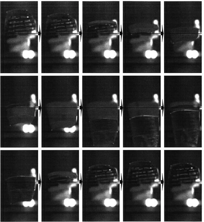
2-10 Video sequence of WASP wing response at 46 m/s and 0' root AOA with 0.006 seconds between images . . . . 22
2-11 Bending response of WASP wing at various speeds and 0' root AOA . . . . . 23
2-12 Bending response of WASP wing at various root AOAs and 46 m/s . . . . . 24
2-13 Video sequence of WASP wing at 46 m/s and -5' root AOA with 0.02 seconds between im ages . . . . 25
2-14 Bending response of WASP wing at 46 m/s and -5' root AOA (corresponding
to case shown in Figure 2-13) . . . . 26
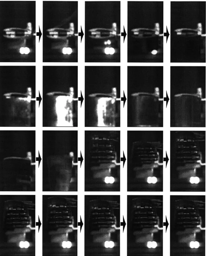
2-15 Video sequence of largest amplitude refold motion captured at 46 m/s and -5 root AOA with 0.04 seconds between images . . . . 27
2-16 Bending response of WASP wing at 46 m/s and 0' root AOA with different segments deflected (refer to Figure 1-5) . . . . 28
2-17 Bending response of WASP wing at 66 m/s and 0' root AOA with different segments deflected (refer to Figure 1-5) . . . . 29
2-18 Typical experimental AOA measurements (taken at 46 m/s and 4' root AOA) 29 2-19 Video sequence of wing deployment at 66 m/s and 00 root AOA with 0.02 seconds between images . . . . 30
3-1 Diagram of double pendulum . . . . 32
3-2 Coordinate systems used in multi-body simulation . . . . 33
3-3 Six-degree-of-freedom finite beam element . . . . 38
3-4 Mesh of wing cross section using quadrilateral elements for use with VABS . 38 3-5 Possible elastic boundary conditions . . . . 40
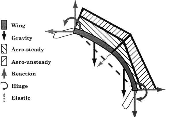
3-6 Loads applied to a flexible segment of a multi-hinge beam structure . . . . . 41
3-7 Photo of tip-most WASP wing hinge showing typical mechanical connections 42 3-8 Bi-linear nature of hinge stiffness . . . . 43
3-9 Possible hinge states . . . . 44
4-1 CPU times for one, two and four elements per wing segment . . . . 55
4-2 Comparison of model with four, two and one element per segment . . . . 56
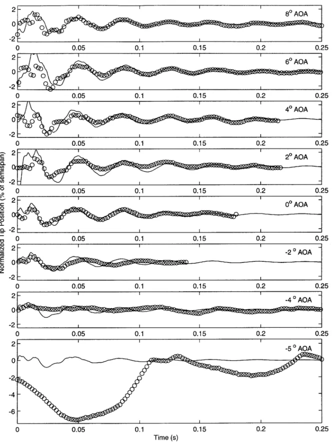
4-3 Wing tip response at various speeds when the root angle of attack is set to 0' 57 4-4 Wing tip response at various angles of attack when flying at 46 m/s . . . . . 58
5-1 Eigenvalue diagram of WASP wing (Uf/wb = 5.65, k = 0.082) . . . . 60
5-2 Eigenvalue diagram of an unhinged wing with WASP properties (Uf/web = 5.12, k = 0.112) . . . . 61
5-4 Normalized mode shape components of one-hinged wing, solid lines for plunge component, and dashed for pitch angle component. . . . . 64
5-5 Characteristics of a one-hinged wing with no second bending flutter instability,
hinge stiffness of 50 Nm (Uf/wab = 5.09, k = 0.103) . . . . 65 5-6 Eigenvalue diagram of a one-hinged wing showing second bending and first
torsion instability, hinge stiffness of 25 Nm (I" bending Uf/Web = 5.25, k =
0.094, 2"d bending Uf/wab = 4.19, k = 0.176 ). . . . . 66
5-7 Eigenvalue diagram of a one-hinged wing with no post second bending
sta-bility, hinge stiffness of 10 Nm (I" bending Uf/web = 5.67, k = 0.073, 2nd
bending Uf/web = 4.51, k = 0.142). . . . . 67 5-8 Map of the one-hinged wing instabilities . . . . 68 5-9 Twist response of WASP wing flying at 210 m/s (flutter speed of 214 m/s)
with 660 N of static lift . . . . 69 5-10 Bending response of WASP wing flying at 216 m/s (flutter speed of 214 m/s)
with 26 N of static lift . . . . 69 5-11 Zoom into one of the cycles shown in Figure 5-10 . . . . 70 5-12 Bending phase projection of WASP wing flying at 216 m/s (flutter speed of
214 m/s) with 26 N of static lift . . . . 70 5-13 Twist response of WASP wing flying at 216 m/s (flutter speed of 214 m/s)
with 26 N of static lift . . . . 71
5-14 Diverging bending response of WASP wing flying at 218 m/s (flutter speed of 214 m/s) with 165 N of static lift . . . . 72 5-15 Diverging twist response of WASP wing flying at 218 m/s (flutter speed of
214 m/s) with 165 N of static lift . . . . 73 5-16 Chaotic bending response of WASP wing flying at 218 m/s (flutter speed of
214 m/s) with 6.5 N of static lift . . . . 74
5-17 Characteristics of a one-hinged wing showing second bending and first torsion instability, '-' stiff state of 22.5 Nm, '- -' soft state of 0.0001 Nm . . . . 75
5-18 Limit cycle oscillation of one-hinged wing flying at 166 m/s (flutter at 165
5-19 Unstable behavior of one-hinged wing flying at 166 m/s (flutter at 165 m/s)
with 309 N static lift . . . . 76
5-20 Divergent behavior of one-hinged wing flying at 175 m/s (flutter at 165) with 60 N static lift . . . . 77
5-21 Limit cycle oscillation of one-hinged wing flying at 150 m/s (flutter at 165) with 44 N static lift . . . . 77
5-22 Limit cycle oscillation of one-hinged wing flying at 135 m/s (flutter at 165 m /s) with 37 N static lift . . . . 78
5-23 Bending response one-hinged wing flying at 160 m/s (flutter at 165 m/s) with 60 N static lift and a -4.7' initial hinge angle . . . . 78
5-24 Bending response of the one-hinged wing flying at 160 m/s (flutter at 165 m/s) with 60 N static lift and a -27.5' initial hinge angle . . . . 79
5-25 Characteristics of a two-hinged wing showing second bending and first torsion instability hinge stiffness of 600 Nm and 26 Nm ( 1" bending Uf/wab = 5.32, k = 0.097, 2"d bending Uf/wab = 5.32, k = 0.161). . . . . 80
5-26 Position and phase of root-most hinge response of two-hinged wing at 140 m/s and 0' AOA (k1 = 600 Nm and k2 = 26 Nm) . . . . 80
5-27 Position and phase of tip-most hinge response of two-hinged wing at 140 m/s and 0' AOA (k1 = 600 Nm and k2 = 26 Nm) . . . . 81
5-28 Steady-state amplitude of torsional response of two-hinged wing with initial conditions in same state and different state than equilibrium . . . . 81
6-1 Unhinged and one-hinged 1-meter span wings (with 30-cm ruler shown for scale) 84 6-2 Diagram of foam wing cross-section . . . . 84
6-3 Eigenvalue diagram of one-hinged wing as designed, '-' stiff hinge (U/web = 1.86, k = 0.436) '- -' soft hinge (Uf/web = 3.77, k = 0.157). . . . . 85
6-4 Photos of foam wing hinge . . . . 86
6-5 Placement of accelerometers in foam wing tip . . . . 88
6-6 Wing hinge with copper contacts . . . . 89
6-8 First two natural frequencies over range of dynamic pressures for the foam wings ('o' unhinged, '*' hinged) . . . . 92
6-9 Mid-chord accelerometer data (solid line) during a hinge-based limit cycle
oscillation of hinged wing at 36.5 m/s and -3' root AOA. Hinge state data
(dotted line) values of less than 50 indicate a partially closed hinge . . . . . 93 6-10 Mid-chord accelerometer data (solid line) during a stall based limit cycle
oscil-lation of hinged wing at 38.6 m/s and 00 root AOA. Hinge state data (dotted line) values less than 75 indicate a soft hinge state . . . . 94
6-11 Mid-chord accelerometer data (solid line) during a stall-based limit cycle
os-cillation of unhinged wing at 38.8 m/s and 00 root AOA . . . . 95 6-12 Steps followed for tip plunge determination, referring to steps outlined in
Section 6.5 for one-hinged wing at 38.6 m/s and 00 AOA . . . . 98 6-13 Comparison of first two natural frequencies of the unhinged wing over range
of dynamic pressures for model (-) and experimental data (*) . . . . 99
6-14 Comparison of first two natural frequencies of the hinged wing over range of dynamic pressures for model (-) and experimental data (*) . . . . 99 6-15 Eigenvalue diagram of one-hinged wing as designed, '-' stiff hinge (Uf/wab =
3.00, k = 0.188), '- -' soft hinge (Uf/web = 2.56, k = 0.264). . . . . 100 6-16 Simulation results for a one-hinged wing flying at 36.5 m/s and a -30 root
AOA subjected to a 0.3-second cosine gust starting at 0.2 seconds . . . 101 A-1 WASP prototype wing . . . 113 E-1 Script logic diagram . . . 127
List of Tables
2.1 Angle of attack performance characteristics of the WASP wing . . . .
6.1 Natural frequencies of stiff state of one-hinged wing as originally designed . Foam wing impulse response (in Hz) . . . .
Operating conditions where a hinge-based limit cycle was recorded . Effect of model tuning factors on wing frequencies . . . . Effect of model tuning on flutter speed (m/s) . . . .
. . . 90
. . . 92
. . . 96
. . . 96
A.1 WASP Wing planform dimensions . . . . A.2 Cross-sectional properties of WASP wing (referenced to elastic axis) A.3 Cross-sectional properties of one-hinge wing . . . . A.4 Experimentally obtained WASP wing hinge properties . . . . Foam wing planform . . . . System parameters of experimental wings . . . . Properties of the Endevco 22 piezoelectric accelerometer Steady state test matrix . . . . Dynamic test matrix, variable speed, 0' AOA . . . . Dynamic test matrix, variable AOA, speed of 45 m/s . . Test points of unhinged foam wing . . . . Test points of one-hinged foam wing . . . . . . . . . 113 . . . . . 114 . . . . . 114 . . . . . 114 . . . . . 117 . . . . . 118 . . . . . 118 119 120 120 121 122 6.2 6.3 6.4 6.5 19 85 B.1 B.2 B.3 C.1 C.2 C.3 C.4 C.5
Chapter 1
Introduction
1.1
Motivation
The idea of using a hinged wing to fulfill space constraints has been around for a number of years. However, most hinged wings have only one joint and are locked in place during operation. There are a number of roles in which it might be useful to have a wing with multiple hinges, or hinges that deploy in flight, or hinges that do not lock. A hinged wing might be used to 'morph' an air vehicle - allowing it to change its wing-spans in mid flight. Another role is remotely deployable vehicles that have extreme packaging constraints, such as the suggested Mars Plane [1] or the Wide Area Surveillance Projectile (WASP) further described below.
1.1.1
Flying Radar Target
A vehicle with a hinged wing that deploys mid-flight has been demonstrated. The Naval
Research Laboratory used a folding wing design for the Flying Radar Target (FLYRT) [2,
3]. The FLYRT vehicle was designed to be stored on a naval ship, and to be compatible with
the shipboard Mk 36 decoy launching system. FLYRT was to be launched with a rocket motor attached and carry advanced electronic warfare payloads.
The wings of the FLYRT vehicle had one hinge and were latched in place when deployed. The main wing section was aligned with the body and pivoted out for deployment. The
(a) Front View
Fuselage
(b) Top Down View Wi"g
IE
I
I
1_I
I
Figure 1-1: FLYRT deployment
outer wing panels were released and would 'fly' into place, shown in Figure 1-1. While several methods involving cables, springs and rods were considered, these were deemed awk-ward and unreliable. It is not known how much, if any, analysis of the aeroelastic effect of the hinges was performed before or after the testing since it was not presented in open literature. However, drop tests of a FLYRT model did prove that gravity and aerodynamic lift alone could deploy those hinged wings. The FLYRT model did have difficulties with nonsynchronous wing deployment causing unrecoverable flight instabilities.
1.1.2
Wide Area Surveillance Projectile
A multi-hinged wing was an integral part in the design of the Wide Area Surveillance
Pro-jectile (WASP) project. The following is a basic overview of the WASP project. A more detailed description of the project can be found in [4, 5].
MIT's Department of Aeronautics and Astronautics and Draper Laboratory began a program in the summer of 1996 utilizing the resources of both to develop a new aerospace system. The objectives of the program were to design a 'first-of-a-kind' system and produce and test a prototype within a two-year time-line. This system needed to provide a solution to a national need or problem. It also had to have an element of 'unobtainium' or high-risk technology.
The first few months of the program were used to create basic system concepts. These concepts were judged on potential marketability, technological innovation, and feasibility of meeting the two-year deadline. The winning concept was WASP, a concept to ballistically deploy an autonomous sensorcraft to a target area.
WASP was sized to be as small as feasible. While it was thought possible to design a system that could be deployed from a soldier's rifle, this was deemed too difficult to achieve. Thus, WASP was sized to be fired from artillery or naval cannons allowing ship captains and artillery commanders near instantaneous reconnaissance of twenty-mile-away target areas. This would fill a niche between that of long duration type Unmanned Aerial Vehicles (UAVs), like the Predator and Global Hawk, and smaller, troop deployable UAVs that were then under development.
In order to successfully fill its market niche, a set of system level requirements was created to guide the design process. These requirements were determined after consulting with officials from the US Army and Navy.
" Compatible with 5-inch Navy gun " Survive a 15,000 g acceleration " Loiter for 15 minutes
* Be autonomous and carry a camera
* Inexpensive and storable for at least three years
" Interact with a ground station and send real-time images and GPS coordinates of
targets
To meet the design requirements, a small UAV was chosen to be the deployable portion of the WASP system. This small flyer would be packaged inside of a modified 5-inch naval shell which normally carried a flare, Figure 1-2. This design would help protect the flight vehicle from the launch environment. It also provided a massive projectile (desirable for long range) and a light flyer (desirable for long endurance.)
EXPLD STATE: SEPARATION
Figure 1-2: Exploded view of WASP and shell
The shell, after leaving the gun, would travel ballistically to the target area. When near the target area, the back end of the shell would separate. A parachute would deploy which would pull the flight vehicle out of the shell and decelerate it to subsonic speeds. The vehicle's engine would start, and the wings and tail would be deployed. Such a scenario is demonstrated in Figure 1-3.
The three major constraints that affected the wing system were the launch loads, size, and loiter time. To achieve a long loiter time, the wings needed to be long and light. A simple unhinged wing large enough to supply the needed lift to the system would not have fit within the allowed space. There was a direct trade off between the space taken up for the wings and the space left for the remaining systems, particularly engine fuel.
Several different concepts were studied for the wings. Telescopic wings were rejected due to the possibility that the sections would jam together under the launch loads. Inflatable wings were deemed too complex to design within the project time-line. Folding wings were chosen due to their simplicity and robustness. Proof of the validity of the concept of a folding wing deployed in flight used on a small UAV came from the Navy's Flying Radar Target
Back End Separation 3 3 Parachute Deployment pration Fin Deployment Wing Unfold/ Controlled Flight C Launch LL Mission
Figure 1-3: WASP mission [5]
discussed in section 1.1.1.
The wing has a constant airfoil shown in Figure 1-4, and the coordinates can be found in Appendix A.2. The thickness of the trailing edge allows the wing to survive the high-g launch loads. The wing is cambered to allow the segments to fold inside of each other. The camber also gives the wing positive lift at low angles of attack which assists in wing deployment and stability.
Figure 1-4: WASP airfoil
The wing is divided into six sections separated by five hinges as shown in Figure 1-5. The wing planform can be found in Appendix A.1. The lengths of the sections and the hinge geometries were sized based to meet the launch requirements. Each wing segment would rest on its hinge, which would, in turn, rest on the hinges underneath. Thus each wing section would only have to carry its own weight. Wing machined from aluminum alloy 7075 were tested under launch accelerations [5].
Even though extensive work was performed on the design, characterization and testing to design the WASP high-g hinged wing, no studies were conducted to assess the aeroelastic behavior of the wing.
LJ
Figure 1-5: WASP wing prototype
1.2
Previous Work
To study the aeroelastic response of a multi-hinged wing, two fundamental problems need to be addressed. The first is multi-body dynamics, and the second is piecewise nonlinear aeroelastics.
Multi-body dynamics models the mechanics of interconnected rigid and elastic bodies. Most multi-body systems are quite complex and non-linear. Several methods are used to solve these systems. One method uses nonlinear finite elements which use direct strain measurements [6]. This technique was specifically tailored toward a system composed of beams connected by hinges. More popular is the use of Hamilton's Principle combined with Lagrangian multipliers to satisfy system constraints [7-9]. This method allows for quick, methodical construction of complex mechanical systems. The dynamics of each of the bodies is determined separately and a series of constraint equations is used to determine the influence of the bodies on each other.
The piecewise nonlinear nature of a multi-hinged wing is similar to that of a control surface with freeplay in that the elastic properties can change dramatically with position. A hinge is either open or closed, and a surface with freeplay is either free or not. The aeroelastic performance of nonlinear structures is an extensive area of research with an abundance of analytical and experimental studies [10-20]. These studies have looked into structures with bilinear stiffness (stiffening and softening), freeplay, and nonlinear stiffness, all of which are illustrated in Figure 1-6. Most of these studies have looked into systems of two or three degrees of freedom with either nonlinear torsional stiffness or flap freeplay as these are the most common occurrences in a typical wing. McIntosh et al. [21] and Hauenstein et al. [22,
23] performed analytical and experimental studies of a system with bilinear and freeplay
10 03 -a0 (a) (b) q "0 0 Position Position (c) (d)
Figure 1-6: Nonlinear stiffnesses (a) cubic, (b) bilinear ('-' stiffening, '.' softening), (c) freeplay, (d) bilinear hinge
wing. A summary of work in nonlinear aeroelasticity was compiled by Lee et al. [24].
A linear aeroelastic system will either have static subsidence or divergence, or a damped or
divergent oscillation. However, the previously mentioned studies have shown that a nonlinear aeroelastic system might also go into a limit cycle oscillation and can exhibit chaotic or nonperiodic behavior. While this type of behavior might be expected of a system with a symmetric nonlinear stiffness, the effect of asymmetric nonlinearity has not been studied. In addition, the effect of multiple bilinear pitch degrees of freedom on a three-dimensional body is unknown.
1.3
Present Work
At the end of the WASP project, the structural performance of the wings subjected to launch loads had been well tested. However, the aerodynamic and aeroelastic performance
were unproven. While the FLYRT had demonstrated unassisted deployment, it had only one hinge. The WASP wing has five hinges and they do not have latches. It was unknown whether these hinges would have a large impact on the aeroelastic performance of the wing. As the wing was to deploy at relatively high speeds, it became important to determine the flutter speed of the wing. It was also unknown how the wing would respond to gust loads or rapid maneuvers.
The objective of this thesis is to study the effects of having multiple unlatched hinges on the aeroelastic performance of a wing. To gain a basic understanding of the flight char-acteristics of hinged wings, the WASP prototype wing was tested in a wind tunnel under various flight conditions. These experiments and their results are described in Chapter 2. The knowledge gained from these flight experiments helped in the development of an an-alytical model designed to predict the behavior of a multi-hinged wing. The development of the model is detailed in Chapter 3. The model is solved in the time domain to capture any nonperiodic motion. Chapter 4 evaluates the ability of the model to capture the fun-damental aspects of the WASP wing in flight. After showing that the analytical model can predict the response of the WASP wing to benign flight conditions, the model was used to explore the full flight envelope of hinged wings. The numerical model predicted that hinged wings exhibit behavior similar to other nonlinear aeroelastic systems such as limit cycle os-cillations and chaotic response. The results of these studies are detailed in Chapter 5. To verify accuracy of the model in predicting the nonlinear response of a hinged wing, a new round of experimental tests were performed on custom built wings. Using the theoretical model developed herein, wings were designed to exhibit characteristics unique to a hinged wing. Their design, experimental setup, and results are presented in Chapter 6. A summary and discussion of all the experimental and analytical results is presented in Chapter 7. This chapter theorizes the fundamental differences between a normal and a multi-hinged wing. It also suggests future work that could gain a better understanding of a multi-hinged wing, and tests that could be done to further verify the proposed theories.
Chapter 2
Experimental Testing of a
Five-Hinged Wing
A prototype wing from the WASP vehicle was used to gain initial insight into the
perfor-mance of a more complex multi-hinged wing. Static and dynamic flight tests were done to determine the low speed flight characteristics of that wing. This data was used to assist in the development of the analytical model described in Chapter 3.
2.1
Wing Characterization
Static loading tests were performed on the prototype WASP wing to determine its physical hinge properties.
To determine the hinge properties for an open hinge, the wing was clamped in an in-verted orientation. Loads were applied by hanging weights at each of the hinge locations. The vertical displacement of several locations was determined using a Questar microscope. Through the microscope, several targets on the wing were monitored during the loading to determine their vertical displacement (see Figure 2-1).
Most of the springs for the WASP prototype were custom made. To determine the stiffness of the springs, the wing was placed on its side and a load was applied to each hinge and to the wing tip one at a time, as schematically shown in Figure 2-2. The load was applied
Targets Weights
Figure 2-1: Schematic of static load testing using Questar microscope
by using a weight attached to a string that was looped over a pulley. The angles of the string
and the segments were measured such that the torque applied could be determined. Only one segment was allowed to deflect at a time by softly clamping the previous segment. A hard clamp resulted in enough wing deformation to impinge the hinge.
Each hinge had a significant amount of static friction, thus two measurements were made for each applied torque. One measurement was taken at the largest angle the spring could maintain for the given torque and the other at the smallest angle. The difference in the angles was the contribution of the static friction. The mean of the two angles is the deflection that would have occurred if there was no static friction.
No experiment was performed to determine the damping or restitution of the hinges. This was partially due to the inability to clamp the individual segments without causing a change in the hinge properties. Other difficulties included the alignments necessary to properly obtain data, and the lack of a quality data acquisition system.
Clamp
Spring
Min. Angle
Max. Angle
Pulley -
-Figure 2-2: Top view of hinge spring measurement setup
2.2
Wind Tunnel Setup
The wing was tested in the Wright Brothers Wind Tunnel at MIT. The low-speed pressurized tunnel has a 3-by-2.3 meter elliptical cross-section and is capable of steady flows up to 90
m/s.
The wing was flown in a horizontal configuration, as shown in Figure 2-3, to orient the gravitational forces correctly. The wing was mounted to a one meter high rigid pedestal. The mount allowed the wing to pivot about its pitch axes, while fixing the yaw and roll axes. The angle of attack (AOA) of the wing was controlled using a pitch arm attached to a screw drive.
2.3
Instrumentation
Static and stagnation air pressure and air temperature were measured using the basic instru-mentation of the wind tunnel. The lift forces on the wing were measured using the tunnel's six-axis force balance.
Figure 2-3: Wing mounted in Wright Brothers Wind Tunnel
system was used to record the position of the wing rather than in-situ sensors. The video system recorded the behavior of the wing at 500 frames per second. The video system's camera was placed outside of the wind tunnel, aligned with and just below the wing's span axis as shown in Figure 2-4. Targets were painted on the wing tip at the leading and trailing edges, and on each of the hinges (Figure 2-5). The data from the camera was stored on VHS videotape and then transferred to digital QuickTime 4.0 format using Adobe Premier 5.0.
2.4
Test Procedure
Prior to testing, the tunnel's force balance was calibrated using a spring scale. The wind tunnel was not stopped between individual tests. The testing concentrated on three areas:
1. Steady state performance
2. Response to disturbance (gust)
3. Deployment characteristics
Figure 2-4: High speed camera position for wind tunnel testing
2.4.1
Steady State Performance
The first set of tests determined the steady state performance of the wing. The test matrix was set up to slowly expand the flight envelope of the wing.
For the WASP wing, high AOA studies were then conducted at the lowest testing speed. The AOA was incremented by single degrees until the lift force started to decrease. For these tests, tufts of yarn were taped to the upper surface of the wing to help visualize the flow reversal near stall.
Low AOAs were studied at the WASP cruising speed (40 m/s). The AOA was decreased
by single degrees until the wing tip oscillations showed large amplitudes.
2.4.2
Response to Disturbance
To explore the unsteady performance of the wing, a series of disturbance tests were per-formed. This was accomplished by placing a rod into the flow and using it to deflect the wing. This method allowed control over which of the hinges were bent by which segment of the wing the rod pushed on. It was decided that the rod should strike the wing swiftly to minimize its impact on the airflow around the wing. This method reduced the amount of control over the initial displacement of the wing, but still regulated which hinge was deflected.
The wing was flown at a constant AOA over a range of speeds. At all of these speeds, the tip-most hinges were disturbed using the rod technique. The disturbance tests were also done at cruising speed of the WASP wing over a range of AOAs. The decay rate of the oscillation of the wing was monitored.
2.4.3
Deployment
Full WASP wing deployment was tested at 70 m/s and zero AOA. This speed was set for safety reasons and is below the design deployment speed of the WASP wing. The wing was completely folded and held in place via an elastic band as shown in Figure 2-6. When the wing was being folded for this test, the inboard most hinge spring became disconnected and was not repaired before the test.
Figure 2-6: Wing folded prior to deployment testing
With the wing folded and held in place, the wind tunnel was brought up to speed. After the wind tunnel had been at test speed for over a minute, the rubber band was released and the wing unfolded.
2.5
Data Postprocessing
The pressure and force data were used to find the coefficient of lift at every test point as, L
CL = L(2.1)
(PT - Ps)A
where L is the lift force of the wing, A is the wing area ( 0.0277 m2
, see Table A.1), and PT and P, are the stagnation and static pressures respectively.
Since there were large temperature differences between some of these data points (as much as 254C), it is believed that this had an effect on the calibration of the force balance. This resulted in large variations in the measured coefficient of lift at various test points with near equal dynamic pressures and AOAs. The force balance had no known correction for temperature. A correction was approximated by finding a correlation between coefficients of
lift and temperature at given dynamic pressures and AOAs.
The QuickTime images made from the high-speed video data were analyzed on a Mac-intosh computer using the public domain NIH Image program [25]. NIH Image allowed the target image's pixel location to be found in each frame of video. Determining the number of pixels between the wing tip targets gave a scaling of 25 pixels per centimeter. When the wing tip went through rapid motion (on the order of hundreds of centimeters per second) the targets would blur. While some blurring could be handled by finding the center of the blurred image, the location of the targets on some frames could not be determined.
2.6
Static Testing
As described in Section 2.1, tip loads were applied to a clamped wing to determine its open hinge properties. Figure 2-7 shows the wing deflection due to static upward bending loads. The deflection was measured at each of the hinges and at points halfway between the hinges. The deformations are largely dominated by bending about the hinge points. The results from this set of experiments allowed the open hinge stiffness and the angle at which the hinge switches states to be determined.
To characterize non-open hinge properties, torque was applied to each of the WASP wing hinges. Two points were measured for each applied torque. The first is the largest hinge angle that could be maintained under the torque, and the second the smallest. From this information the hinge spring stiffness and static friction could be approximated. Figure 2-8 shows the results of this set of experiments. A best linear fit was found to both the higher
and lower displacement data sets. The slopes and intercepts of the two linear fits were averaged together (weighted by the number of data points) to give the hinge stiffness curve. The difference in the intercept between the averaged line and the curve fits gives the static friction of the hinge. The hinge characteristics are summarized in Appendix A, Table A.1.
3.5 Tip Load 3- - 0N - 4.6N 2.5- ~... 9.1N -- - 13.5 N -0 0.5- 0-15 20 25 30 35 40 45 Span Location (cm)
Figure 2-7: WASP wing deformation at hinges (o) and mid segment (U) due to static tip loads (open hinge configuration)
2.7
Steady State Response
During the dynamic phase of testing of the WASP wing, the steady state values of lift were obtained before the wing was perturbed. This data was combined with the data gathered during the steady state phase of testing to determine the flight characteristics of the wing.
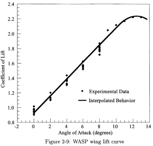
Figure 2-9 summarizes the lift results corrected for temperature obtained during both phases of testing. The expected behavior line is an estimate of the experimental lift curve. The experimental data was used to determine the angle of attack required during cruise. This is the angle at which the wing would need to operate such that, at the cruise velocity, they could support the weight of the WASP vehicle. As shown in Table 2.1, the cruise angle of attack was close to the angle predicted [5]. Table 2.1 also shows the angle of attack at which stall was recorded. Stall was determined by a peak in the lift curve as well as by observing flow reversal on the wing.
x 10-3 10 - 8- 6-4 Hinge E/F 0 10 20 30 40 50 60 70 0.025-0 .0.025-0 2- .... --... -... 0 .0 1 5 - .-- -- --. -... --....~ 0.01 5 0.005 .. --- ~~Hinge D/E -0 10 20 30 40 50 60 70 E Z 0.15 -- - ~ C D... L 0.1 - 0>0.05-C: 0 10 20 30 40 50 60 70 0.2 --0. - - -~-~ Hinge B/C CL I I I I I 0 10 20 30 40 50 60 70 0.2-0 1 - ... ... ... ... 0 .1 -. -- - -- ' 'H in g e A / B 0 10 20 30 40 50 60 70
Hinge Angle (degrees)
Figure 2-8: WASP hinge spring measurements (*) with stiffness curve (-) and stability boundaries (- -)
2.4 2.2 2.0 1.8 0 1.6 S1.4-0 U 1.2 + Experimental Data - Interpolated Behavior 1.0 0.8 I -2 0 2 4 6 8 10 12 14
Angle of Attack (degrees) Figure 2-9: WASP wing lift curve
Table 2.1: Angle of attack performance characteristics of the WASP wing Predicted Cruise AOA 5.50
Experimental Cruise AOA 6'
Experimental Stall AOA 120
2.8
Dynamic Response
To study the dynamic response of hinged wings, the wing was flown in a variety of flight conditions and the behavior of the wing was monitored. The wing segments had to be manually disturbed to provide a large enough response for the camera system to measure.
The dynamic testing phase of the WASP wing experiments examined the nonlinear re-sponse of hinged wings in flight by perturbing the wing in such a manner that at least one of the hinges would switch from the stiff to the partially closed state.
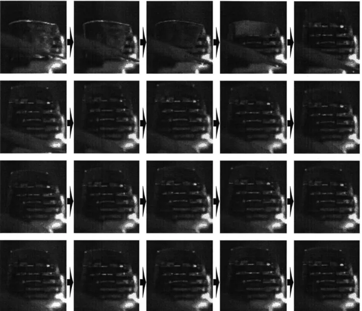
The high-speed video system was able to capture the motion of the tip of the wing as shown in Figure 2-10. However, some experiments caused the wing tip to move too fast.
This nominally occurred just after the tip was deflected. Moreover, at times (such as the deployment test or a large amplitude oscillation) the tip would move out of the field of view of the camera.
Using the NIH Image program results in accuracy of approximately one pixel. There are
96 pixels from the center of the leading edge target to the center of the trailing edge target,
a distance of 3.81 cm. The vertical location of the wing tip was found by averaging the location of the wing tip targets. Therefore, the height of the wing tip was found with an accuracy of ±0.02 cm, or t0.05% of the semi-span.
While testing in the wind tunnel, the tip of the wing would oscillate at all flow speeds even when unperturbed. This oscillation was most likely due to a non-uniform wind tunnel flow. The broad band forcing of the non-uniform flow caused the wing to oscillate at its natural frequencies. It is possible that the frequency of the non-uniform flow could have been biased toward the tunnels fan frequency.
Figures 2-11 and 2-12 summarize the vertical locations of the wing tip during the dynamic testing where the wing tip is intentionally perturbed. The origin of the time axis is defined when the tip crosses the steady state value. The vertical tip locations are measured with respect to the steady state tip location for the flow condition. Each test had a different initial condition, thus the amplitude of the responses cannot be directly compared. The oscillations due to the disturbance were not much larger than the natural oscillations due to the tunnel noise for more than three or four cycles. These oscillations would occur at about
25-30 Hz. This gives less than 80 frames of data before the noise of the tunnel overcame the
response. That is not enough of a sample to accurately determine the response frequency of the system. However, a few trends can be seen in the experimental data.
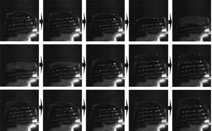
The frequency of the response does have a slight, but noticeable, increase as free stream speed is increased. Speed increase also causes a faster decay of the transient response. An increase in the root angles of attack tends to cause an increase in the response amplitude. However, this trend reverses for very low angles of attack, as can be seen in Figure 2-13 (only looking at every 1 0th frame). Here the wing enters the 'refold' condition. Figure 2-14 shows
data generated by analyzing all the frames of data of the sequence shown in Figure 2-13. Figure 2-15 shows the largest oscillation observed at this flight condition. While the tip of
the wing goes outside of the video frame, it is estimated that the tip plunges as much as
30% of the semi-span.
Deflecting more than just the tip segment changed the wing response as can be seen in Figures 2-16 and 2-17. In Figure 2-16 the wing tip motion dips into a smooth curve implying that one of the wing hinges had changed states. Unfortunately, the targets which were used to measure the position of the wing along the span were placed on the under-side of the wing. Thus, the targets were blocked by the tip segment during the time just after the disturbance.
By the time the targets were visible, most of their motion had been damped out.
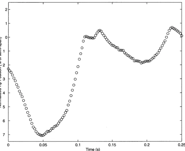
The tip twist angle of the wing oscillated at too high of a frequency and too low of an amplitude to be accurately measured by the high-speed video system. A simple finite element model of a similar hingeless (WASP) wing found the first torsion mode would occur at about 210 Hz. The video system sampled at a rate of 500 frames per second giving less than three samples per expected cycle. The tip twist angle was determined by measuring the difference in height of the targets on the leading edge and trailing edge of the wing tip. This system has an accuracy of approximately t0.5*. Figure 2-18 is a plot of a typical tip twist angle as seen by the video system
The wing deployed as expected, even without the inner-most hinge spring. Figure 2-19 shows the video footage of the deployment. It appeared that the wing did straighten out in all but the inner-most hinge first. It then quickly pivoted around the inner-most hinge until it was in a normal flight orientation.
Unfortunately, no instrumentation was available at the time to provide a real time analysis of the lift force of the WASP wing. However, the high-speed video system could measure the time from release to fully open (0.23 seconds), and the additional time until the deployment induced motion became negligible (about 0.3 seconds).
Figure 2-10: Video sequence of WASP wing response at 46 m/s and 0' root AOA with 0.006 seconds between images
* 50.9 m/s co~ 55.6 rn/s 0. 1.5 I5 E 0. 01 -I. ~0 0.54 -o E -1.5 - -0 -2---2.5 0 0.05 0.1 0.15 0.2 0.25 Time (s) I Error 0 60.3 mn/s 2 -* 0 65.6 m/s-* 70.7 rn/s 1.50 0. 0 0O z -2 -2.5 0 0.05 0.1 0.15 0.2 0.25 Time (s)
2.5 1 * 0AOA E CO, 1 - - 0.5-o *-0 ~0 NL * -10.5 -o --0 z --2.5 0 0.05 0.1 0.15 0.2 0.25 Time (s) 2.5 I Error 0 20 AOA 2 0 40 AOA C. 15* 60 AOA a- 1.5-- > 80 AOA E a 1 -0.5 0 -0.5 o z 0 -2 0 ** -2.5 0 0.05 0.1 0.15 0.2 0.25 Time (s)
Figure 2-13: Video sequence of WASP wing at 46 m/s and -5' root AOA with 0.02 seconds between images
2 1 C El ai) 0 C 0 5) 0 a. 3 0 z 5 0J 6 7 0 0.05 0.1
Figure 2-14: Bending response of WASP to case shown in Figure 2-13)
Time (s)
0.15 0.2 0.25
wing at 46 m/s and -5' root AOA (corresponding
0 0 00 0 0 00 0 0 0 00 00 o0 0 0 o 0 o0 o 0 0 o 09 0 0 0 0
Figure 2-15: Video sequence of largest amplitude refold motion captured at 46 m/s and -5' root AOA with 0.04 seconds between images
0 Segment F 2 0 Segment E 0 * Segment D 0 -O 0 o C4 C 0n *0 0 00 5 0 . .50202 -0 0 NL. 0 0 00 00 -3 0E 00 -4 0 0.05 0.1 0.15 0.2 0.25 Time (s)
Figure 2-16: Bending response of WASP wing at 46 m/s and 00 root AOA with different
3 C CL E 0 M 00 o oo0 CD 0. 00 L -Of ** -~ 0 CO 0 00 - 0 z -2 - Eib -3 0 0.05 0.
Figure 2-17: Bending response of WAS segments deflected (refer to Figure 1-5)
0.25
1 0.15 0.2
Time (s)
P wing at 66 m/s and 00 root AOA with different
0 0 0 0 0 0 OC9 % 000 0 0 0 0 00 0 U 0 oo 0 0 0 0 00o 0 00 00 O 0000 06C 0 0 0 00 0 00 0 0 0 0.05 0.1 0.15 Time (s)
Figure 2-18: Typical experimental AOA measurements (taken at 46 m/s and 40 root AOA) 5.51 0 0 0 09 ~00 5 04.5 4 0 (D 3.5 3L 3 0 0 0 0 0.2 0.25
*
I
Q
Figure 2-19: Video sequence of wing deployment at 66 m/s and 0* root AOA with 0.02 seconds between images
Chapter 3
Theoretical Modeling
A nonlinear aeroelastic model was created to simulate a multi-hinged wing at different flight
conditions. It is able to handle both the large hinge angles and the piecewise stiffness found in a hinged system. The inputs of the model include the wing cross-sectional properties (geometric, structural and aerodynamic), the number of wing segments, the mechanical properties of the hinges, and the flow parameters. Using a direct time marching scheme, the model determines the change in state of the wing over time.
The model was developed by initially simulating a dynamic system with multiple rigid bodies. Next, the forcing terms were added one at a time using models that were indepen-dently verified. The aerodynamic model, as well as the integration schemes, were based on methods used by Conner et al. [17].
3.1
Multi-Body Dynamics
The multi-body dynamics are modeled using the methods developed by Shabana [7] which uses Lagrangian multipliers to satisfy system constraints. In order to create a full wing model, a double pendulum problem is used to exemplify its development. The double pendulum is a classic chaotic problem [26] with two rigid beams connected end-to-end by a pin joint. The unconnected end of one of the beams is pinned in space as shown in Figure 3-1. A hinged wing consists of a number of elastic beams connected by pin joints, of which one of the most
Figure 3-1: Diagram of double pendulum
inboard segment has its unconnected end clamped in space.
For a system of rigid beams connected by pin joints constrained to move in a plane, only one degree of freedom (DOF) is needed to describe the state of each beam. However, to simplify the process when doing large numbers of connected beams, three DOFs are used, of which only one is independent. A system of constraint equations is used to define the relationships between the dependent and independent DOFs.
Two sets of coordinate systems are used to describe the state of the system (Figure 3-2). The first (X,Y) is a single inertial frame that is common to all bodies. The second set of frames (xi, yi) consists of local frames that are each attached to a body and can translate and rotate with respect to the inertial frame. For this discussion i is used to distinguish each body frame and and
j
is used to specify the jth point or element on the ith body. Any arbitrary point in the inertial coordinate system can be described by the position vector, rij, which can be determined by:rij= Ri + Aiuij (3.1)
where Ri is the location vector of the origin of the body coordinate frame in the inertial coordinate system. For the double pendulum, the body coordinate systems are placed at the root of the beams to simplify the formulation that will be encountered when elastic beams are considered. uij is the location vector of the jth point in the ith body coordinate system.
Y
x. -yi
ei
/i
x
Figure 3-2: Coordinate systems used in multi-body simulation
by: cos(64) sin(61) - sin(6i) cos(j) (3.2)
where 92 is the rotation angle of the ith body with respect to the inertial frame. Thus, the state of a rigid body can be described using the vector qj, i.e.,
qj =
I
I
(3.3)The change of rij over time can be found by differentiating Equation 3.1, that is
rAj - -r7,=_ R. u Ao 0
80s
- sin( ) cos(0j) (3.4a) (3.4b) - cos(6) - sin(00)J
Using the virtual work, 6W, done by all forces, F, acting on the system, a vector of and
generalized forces
Q
can be found through:6W = F Tr = QT6q (3.5)
where
oq
is a vector of system virtual displacements. The vector of generalized forces can be used in Lagrange's Equation to determine the equations that describe the motion of body i throughd (IT \T IT T
~H\\4J ~ =j
Q-(3.6)
dt 0qi Oqj
where T is the total kinetic energy of the system and
Qj
is the portion ofQ
related to 6q., the virtual displacements of the ith body.The total kinetic energy of the system is the sum of the kinetic energy of each body, Ti. The kinetic energy of the ith body is given by
T =
I
p.T sijd (3.7)2Vol,
where p is the density of the body and can be a function of location. Using Equation 3.4a in Equation 3.7, a matrix Mi can be defined from:
1 T
Ti = -A MA (3.8)
2
Mi can be separated into its subcomponents MRR I MRO, and M6 ." The subindex R refers
to a rigid body translation, and the subindex 0 refers to rigid body rotation. Thus MRO is the subcomponent of Mi which is the influence on rigid body translations due to rigid body rotation. These subcomponents are found by expanding the above equation giving,
I AOeu1
[
MRR M RGMi = p
dV
= (3.9)vo (Ao, uij) uL M M
where I is the identity matrix.
A double beam pendulum consists of beam-like bodies. The assumptions that the length
for the mass matrix subcomponents of the double beam pendulum to be determined by:
MRR pIdV = [i (3.10a)
Ri - si01 m0 l in0
M R =
f
pxi sin6O dV = sin (3.10b)vol cos
f
2 cos 9M,,=
Vol
dV= (3.10c)where mi is the mass of the ith body. For a body with the coordinate system placed at the center of mass, the MRO2 terms would be zero. For the case of the double pendulum, the
local coordinate systems are placed at the root of the beams, which leads to the mass matrix having off-diagonal terms. Note that MRO6 has state variables, thus the model is nonlinear.
The system can be written in the form az = b by placing Equation 3.8 into Equation 3.6 and using the convenient forcing term
Q,,,
that isMAd + Miqi - ciTMii =
Q,
(3.11a)M =
Qi
+Qvi
(3.11b)Qvi
is found by solving its two parts separately, and then finding their sum. As shown in Equation 3.12b, due the mass matrix being independent of the translation terms, the derivative of T with respect to R is zero. Therefore, the first two terms of the second partare zero.
0 0Os
bno
0? Cos i06 i sin 0; 4i= sin 64 (3.12a)