HAL Id: hal-02623557
https://hal.inrae.fr/hal-02623557
Submitted on 26 May 2020
HAL is a multi-disciplinary open access
archive for the deposit and dissemination of
sci-entific research documents, whether they are
pub-lished or not. The documents may come from
teaching and research institutions in France or
abroad, or from public or private research centers.
L’archive ouverte pluridisciplinaire HAL, est
destinée au dépôt et à la diffusion de documents
scientifiques de niveau recherche, publiés ou non,
émanant des établissements d’enseignement et de
recherche français ou étrangers, des laboratoires
publics ou privés.
measurements of evapotranspiration over hilly crop fields
Nissaf Boudhina, Rim Zitouna, Insaf Mekki, Frédéric Jacob, Netij Ben
Mechlia, Moncef Masmoudi, Laurent Prevot
To cite this version:
Nissaf Boudhina, Rim Zitouna, Insaf Mekki, Frédéric Jacob, Netij Ben Mechlia, et al.. Evaluating
four gap-filling methods for eddy covariance measurements of evapotranspiration over hilly crop fields.
Geoscientific Instrumentation, Methods and Data Systems Discussions, European Geosciences Union
2018, 7 (2), pp.151-167. �10.5194/gi-7-151-2018�. �hal-02623557�
https://doi.org/10.5194/gi-7-151-2018
© Author(s) 2018. This work is distributed under the Creative Commons Attribution 4.0 License.
Evaluating four gap-filling methods for eddy covariance
measurements of evapotranspiration over hilly crop fields
Nissaf Boudhina1,2, Rim Zitouna-Chebbi3, Insaf Mekki3, Frédéric Jacob1,3, Nétij Ben Mechlia2, Moncef Masmoudi2, and Laurent Prévot3
1LISAH, IRD, INRA, Montpellier SupAgro, University of Montpellier, 34060 Montpellier, France 2Institut National Agronomique de Tunisie (INAT)/Carthage University, Tunis, Tunisia
3Institut National de Recherche en Génie Rural, Eaux et Forêts (INRGREF)/Carthage University, Ariana, Tunisia
Correspondence: Rim Zitouna-Chebbi (rimzitouna@gmail.com)
Received: 4 August 2017 – Discussion started: 1 December 2017
Revised: 10 April 2018 – Accepted: 14 May 2018 – Published: 7 June 2018
Abstract. Estimating evapotranspiration in hilly watersheds is paramount for managing water resources, especially in semiarid/subhumid regions. The eddy covariance (EC) tech-nique allows continuous measurements of latent heat flux (LE). However, time series of EC measurements often expe-rience large portions of missing data because of instrumental malfunctions or quality filtering. Existing gap-filling meth-ods are questionable over hilly crop fields because of changes in airflow inclination and subsequent aerodynamic proper-ties. We evaluated the performances of different gap-filling methods before and after tailoring to conditions of hilly crop fields. The tailoring consisted of splitting the LE time series beforehand on the basis of upslope and downslope winds. The experiment was setup within an agricultural hilly wa-tershed in northeastern Tunisia. EC measurements were col-lected throughout the growth cycle of three wheat crops, two of them located in adjacent fields on opposite hillslopes, and the third one located in a flat field. We considered four gap-filling methods: the REddyProc method, the linear regres-sion between LE and net radiation (Rn), the multi-linear re-gression of LE against the other energy fluxes, and the use of evaporative fraction (EF). Regardless of the method, the splitting of the LE time series did not impact the gap-filling rate, and it might improve the accuracies on LE retrievals in some cases. Regardless of the method, the obtained accura-cies on LE estimates after gap filling were close to instrumen-tal accuracies, and they were comparable to those reported in previous studies over flat and mountainous terrains. Over-all, REddyProc was the most appropriate method, for both gap-filling rate and retrieval accuracy. Thus, it seems
possi-ble to conduct gap filling for LE time series collected over hilly crop fields, provided the LE time series are split be-forehand on the basis of upslope–downslope winds. Future works should address consecutive vegetation growth cycles for a larger panel of conditions in terms of climate, vegeta-tion, and water status.
1 Introduction
Hilly watersheds are widespread within coastal areas around the Mediterranean basin, as well as in eastern Africa, India, and China. They experience agricultural intensification since hilly topographies allow water-harvesting techniques that compensate for precipitation shortage (Mekki et al., 2006). Their fragility is likely to increase with climate change and human pressure, especially as water scarcity already limits crop production. In this context, understanding evapotranspi-ration processes within hilly watersheds is paramount for the design of decision support tools devoted to water resource management (McVicar et al., 2007). Indeed, evapotranspira-tion (or latent heat flux, LE) directly drives biomass produc-tion through intertwining with photosynthesis (Olioso et al., 2005), and it is a major term of water balance, up to two-thirds of the annual water balance for semiarid/subhumid Mediterranean climates (Montes et al., 2014; Moussa et al., 2007; Yang et al., 2014).
Using evapotranspiration measurements for environmental and water sciences requires complete time series of LE at the hourly timescale, to be next converted into daily, monthly, or
annual values (Falge et al., 2001a, b). This is a prerequisite for long-term studies in relation to global change, but also for short-term studies in relation to agricultural issues and modeling challenges. However, common time series of eddy covariance (EC) measurements, which are today considered to be the reference method, include missing data because of experimental troubles such as power failures or instrumental malfunctions. Also, unfavorable micrometeorological condi-tions lead to the rejection of significant parts of data that do not fulfill theoretical requirements for EC measurements. Statistical studies based on long-term measurements suggest that missing data rates range from 25 to 35 % (Baldocchi et al., 2001; Falge et al., 2001a; Law et al., 2002), while data rejection rates through quality control range from 20 to 60 % (Papale et al., 2006). Therefore, gap-filling methods are nec-essary to obtain continuous time series of land surface energy fluxes.
Most existing gap-filling methods are devoted to carbon dioxide (CO2) measurements (Aubinet et al., 1999; Falge
et al., 2001a; Goulden et al., 1996; Greco and Baldocchi, 1996; Grünwald and Bernhofer, 1999; Moffat et al., 2007; Reichstein et al., 2005; Ruppert et al., 2006). Table 1 sum-marizes the few studies that addressed measurements of LE, along with underlying methodologies and resulting perfor-mances. Prior to gap filling, time series are often split in dif-ferent ways according to the experimental conditions (e.g., nighttime or daytime, wind directions, vegetation phenology, weekly or monthly time windows), so that missing data are filled with observations collected in similar conditions for micrometeorology, vegetation phenology, and water status. Overall, gap-filling methods for LE time series have been evaluated over flat, hilly, and mountainous areas. However, the existing studies for hilly areas did not address their spe-cific conditions (Hui et al., 2004), or were restricted to one gap-filling method (Zitouna-Chebbi, 2009).
Gap-filling methods for LE have to be designed in ac-cordance with the terrain characteristics that impact evapo-transpiration. Conversely to flat terrains that correspond to a slope lower than 2 % (Appels et al., 2016), solar and net radi-ations within sloping terrains change depending on slope ori-entation, with larger values for ecliptic-facing slopes (Holst et al., 2005). Over sloping terrains, the conditions of topog-raphy, atmospheric stability, and airflow within the atmo-spheric boundary layer differ between hilly areas and moun-tainous areas (Dupont et al., 2008; Hammerle et al., 2007; Hiller et al., 2008; Prima et al., 2006; Raupach and Finnigan, 1997). Most existing gap-filling methods rely on covariation of convective fluxes with meteorological variables, or tem-poral autocorrelation of the convective fluxes. Within hilly areas, these relationships are likely to change with wind di-rection and vegetation development because of changes in airflow inclination (Zitouna-Chebbi et al., 2012, 2015), and therefore changes in aerodynamic properties (Blyth, 1999; Rana et al., 2007).
In the context of obtaining continuous time series of evap-otranspiration from EC measurements of LE, the current study aimed to examine and compare LE gap-filling methods over hilly crop fields. For this, we evaluated the performances of different methods before and after tailoring to the condi-tions of hilly crop fields. We used the following methodolog-ical framework.
The experiment was set within a Tunisian agricultural hilly watershed with rainfed crops. It included the data collection and preprocessing, the analysis of the experimental condi-tions, and the analysis of the dataset to be filled.
We considered several gap-filling methods that differ in the use of ancillary information, either micrometeorological data or energy flux data other than LE. Given the possible influence of airflow inclination, the gap-filling methods were tailored by splitting the dataset on the basis of airflow incli-nation as driven by wind direction.
We assessed the performances of the gap-filling methods by addressing (1) filling rate as compared to missing data after preprocessing, (2) retrieval accuracy on filled data, and (3) quality of gap-filled time series through energy balance closure.
2 The experiment: study site and materials
2.1 Experimental site
The Lebna watershed is located on the Cap Bon Peninsula, northeastern Tunisia. It extends from the Jebel Abderrah-mane to the Korba Laguna, and it includes the Kamech wa-tershed (outlet at 36◦5203000N, 10◦5203000E, 108 m above sea
level – m a.s.l.) that has an area of 2.7 × 0.9 km2 (Fig. 1). The El Gameh wadi crosses Kamech from the northeast to the southwest. A hilly dam (140 000 m3 nominal capacity) is located at the watershed outlet. The Kamech watershed belongs to the environmental research observatory OMERE (French acronym for Mediterranean Observatory of Water and Rural Environment, http://www.umr-lisah.fr/omere, last access: 1 April 2018).
The climate of the Kamech watershed is subhumid Mediterranean. Over the 1995–2014 period, cumulated val-ues at the yearly timescale for precipitation and Penman– Monteith reference crop evapotranspiration (Allen et al., 1998) are 624 and 1526 mm, respectively. Terrain eleva-tion ranges from 94 to 194 m a.s.l., and terrain slopes range between 0 and 30 %, the quartiles being 6, 11, and 18 % (Zitouna-Chebbi et al., 2012). The soils have sandy-loam textures, and soil depth ranges from a few millimeters to 2 m according to both the location within the watershed and the local topography. These swelling soils exhibit shrinkage cracks under dry conditions during the summer (Raclot and Albergel, 2006).
Within the Kamech watershed, agriculture is rainfed, tra-ditional, and extensive (Mekki et al., 2006). The main crops
Table 1. Summary of relevant studies that deal with the performances of different gap-filling methods for LE time series. Landform classifi-cation includes flat, mountainous, and hilly. Dataset splits are based on time window or on specific regimes. NR stands for “not reported”.
Study reference Datasets or site Locations/landform/vegetation Boundary layer conditions/wind regimes Dataset split
Gap-filling methods Key results
Falge et al. (2001b)
EUROFLUX and AmeriFlux
– 18 sites/mountainous/four vegetation groups (conifers, deciduous forests, crops, grassland) – NR/NR
– Time window (15 days)
Mean diurnal variation (MDV) Lookup tables (LUTs)
Good gap-filling performances. The two methods performed similarly; MDV estimates slightly overestimated by LUT ones. Cleverly et al. (2002) Sevilleta and Bosque del Apache NWR
– Two sites/NR/woody species – Extremely stable/NR – Time window (daily basis)
LE = a Rn + b
bsignificantly different from 0
NR
Hui et al. (2004)
AmeriFlux – Three sites/hilly topography/forest (deciduous, coniferous, subalpine)
– NR/NR
– No split (1-year dataset)
Imputation methods Good gap-filling performances. The methods performed similarly; multiple imputation method is easily portable in the context of worldwide networks. Alavi et
al. (2006)
NR – One site/flat/winter wheat – NR/NR
– Time windows according to the used method (1 year/4–15 days/±10 days/±10 days)
Kalman filter
Multiple imputation (MI) Mean diurnal variation (MDV) Multiple regressions
Good gap-filling performances of Kalman filtering approach with smaller errors than the other methods. Roupsard et
al. (2006)
NR – One site/flat/coconut plantation – NR/NR
– Time window (1 month)
LE = a Rn + b MDV to gap filling H
NR
Beringer et al. (2007)
FLUXNET – One site/flat/woodland and open forest savanna – NR/NR
– NR
Feed-forward back propagation (BPN) artificial neural network (ANN) (Papale et Valentini, 2003)
NR
Zitouna-Chebbi (2009)
ORE OMERE – Three fields/hilly/winter cereals
– Neutrality or low instability/externally driven – Based on upslope/downslope airflows (1-year dataset)
LE = a Rn + b Good gap-filling performances when discriminating between the two prevailing wind directions. Abudu et
al. (2010)
Bosque del Apache NWR
– One site/NR/salt cedar trees – NR/NR
– Random split for calibration/testing over X % of existing data with X = [5, 10, 20, 30, 40].
Feed-forward (FF) artificial neural networks (ANN) with different in-puts
Best performance with the following inputs: daily maximum and minimum temperature, daily solar radiation, day of the year.
Chen et al. (2012)
NR – One site/mountainous/forest (evergreens and hardwoods)
– NR/NR
– Based on nighttime and daytime (2-year dataset)
Two multivariate methods: – multiple regressions (MRS) – K-nearest neighbors (KNNs)
KNN performed better than MRS.
Eamus et al. (2013)
NR – One site/flat plain/Savanna woodland – Nocturnal stability/NR
– 10-day windows
Self-organizing linear output (SOLO) artificial neural network (ANN)
NR
This study ORE OMERE – Three fields/hilly/winter cereals
– Neutrality or low instability/externally driven – Based on vegetation phenology, and
upslope/downslope airflows (one crop growth cy-cle)
REddyProc (MDV–LUT based) Linear regression method (LE–Rn) Multiple linear regression (MLR) Evaporative fraction (EF)
See results and discussion in the current paper.
are winter cereals (barley, oat, triticale, wheat) and legumes (chickpeas, fava beans). Land use and parcels are strongly re-lated to topography and soil quality. The watershed includes 273 plots, the sizes of which range from 0.08 to 13.65 ha (0.62 ha on average, with a standard deviation of 1.05 ha).
2.2 Measurement locations and experimental period
Three flux stations simultaneously collected measurements of energy fluxes and meteorological variables within three wheat crop fields (Fig. 1): two sloping fields (A, B) and a flat field (C).
Field A was located on the northern rim of the Kamech watershed. It had a fairly homogeneous terrain slope (6◦) that
faced south-southeast and a 1.2 ha area. Field B was adjacent to field A, on the opposite hillside. It also had a homoge-neous slope (5.2◦) that faced north, and it had a 1 ha area. Fields A and B were separated by the northwestern limit of the Kamech watershed. Field C was located in the southeast-ern part of the Kamech watershed. It had a flat terrain and a 5 ha area. A meteorological station (labeled M in Fig. 1) was located near the watershed outlet.
The experimental period started at the beginning of De-cember 2012 and ended mid-June 2013. It thus covered the full growth cycle within the three wheat crop fields, from
ORE OMERE A B C M 0 1 00 km (a) (b)
Figure 1. Location of the Kamech watershed within the Cap Bon Peninsula, northeastern Tunisia (a). Kamech has a 0.9 km width and a 2.7 km length. Three-dimensional view of Kamech (b), including locations of the experimental fields (A, B, C) and of the standard meteorological station (M).
sowing (1 December) to harvest (15 May for field A, 19 June for fields B and C).
2.3 Instrumental equipment and data acquisition
On fields A, B, and C, each flux station collected measure-ments of the land surface energy fluxes: net radiation (Rn), soil heat flux (G), and sensible (H ) and latent heat (LE) fluxes. Table 2 displays the type of instruments used for each flux station along with acquisition and storage frequencies, and sensor accuracies according to manufacturers.
The sonic anemometers, krypton hygrometers, and air temperature and humidity probes were installed at con-stant heights above ground level: 1.98 m for field A, 2.0 m for field B, and 2.2 m for field C. The verticality of the sonic anemometers was carefully checked during the exper-iment with a spirit level, as described by Zitouna-Chebbi et al. (2012). The latter reported a 1◦ accuracy on sonic anemometer verticality, according to the experimental proto-col and to the analysis of airflow inclination. To avoid water ponding on mirrors of the krypton hygrometers, we rotated them in their mounts so that the mirrors were vertical and the measurement path was horizontal. The net radiometers were installed at 1.7 m height above ground level and their horizontality was also checked regularly. For each flux sta-tion, three soil heat flux sensors were distributed a few me-ters around the station, and they were buried at 5 cm below the soil surface.
Measurements at the meteorological station included (1) solar irradiance with a SP1100 pyranometer (Skye, UK); (2) air temperature and humidity with a HMP45C probe (Vaisala, Finland); (3) wind speed with an A100R anemome-ter (Vector Instruments, UK); and (4) wind direction with a W200P wind vane (Vector Instruments, UK). The instru-ments were installed at 2 m above ground level (1 m for the pyranometer). All instruments were connected to a CR10X data logger (Campbell Scientific, USA) that calculated and
stored the 30 min averaged values from the 1 Hz frequency measurements.
All instruments were manufacturer calibrated. Hereafter in the paper, we focus on daytime measurements since LE flux is insignificant (small) during nighttime.
2.4 Data processing: calculation of net radiation and soil heat flux
On fields A and B, the measurements of Rn were corrected for the effect of slope following the procedure proposed by Holst et al. (2005). Details are given in Zitouna-Chebbi et al. (2012, 2015). Only direct solar irradiance was corrected by accounting for the angle between solar direction and the normal to local topography. Direct solar irradiance was em-pirically derived from total solar irradiance measured at the flux station. We characterized local topography with slope (topographical zenith with nadir as origin) and aspect (topo-graphical azimuth with north as origin), both derived from a 4 m spatial resolution digital elevation model (DEM) ob-tained with a stereo pair of IKONOS images (Raclot and Albergel, 2006). The correction for slope effect on Rn was about 50 W m−2on average.
For each flux station, G was estimated by averaging the measurements collected with the three soil heat flux sensors. We did not apply any correction for heat storage between the surface and the sensors for several reasons. First, the existing solutions are questionable when considering swelling soils that exhibit shrinkage cracks under dry conditions during the summer since they require detailed and stable experimen-tal protocols (Leuning et al., 2012). Second, the experiment lasted throughout wheat growth cycles without any flood events that are critical for heat storage correction. Third, ne-glecting the heat storage in the soil above the heat flux plates induces errors on soil heat flux estimates that are not system-atically large since they range between 20 and 50 W m−2on average (20–50 % relative to measured value), as reported by Foken (2008).
2.5 Data processing: calculation of convective fluxes
Hand LE were calculated from the 20 Hz data collected by the sonic anemometers and the krypton hygrometers, using the ECPACK library version 2.5.22 (Van Dijk et al., 2004). Hand LE fluxes were calculated over 30 min intervals.
2.5.1 Flux calculation
Most of the instrumental corrections proposed in the afore-mentioned version of the ECPACK library were applied. These corrections addressed (1) the calibration drift of the krypton hygrometers using air humidity and temperature measured by the HMP45C probes, (2) the linear trends over the 30 min intervals, (3) the effect of humidity on sonic anemometer measurement of temperature, (4) the hygrom-eter response for oxygen sensitivity, (5) the mean vertical
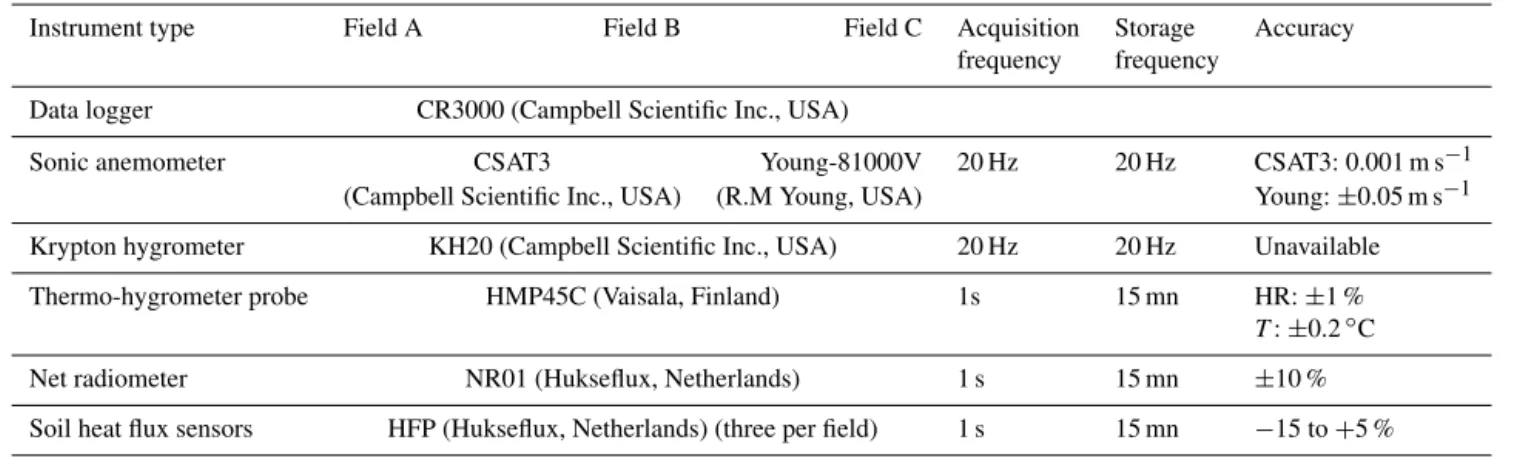
ve-Table 2. Details about experimental setup for each of the three flux stations: type of sensors used, acquisition and storage frequencies, and accuracies as given by manufacturers. HR and T stand for air relative humidity and temperature.
Instrument type Field A Field B Field C Acquisition Storage Accuracy frequency frequency
Data logger CR3000 (Campbell Scientific Inc., USA)
Sonic anemometer CSAT3 Young-81000V 20 Hz 20 Hz CSAT3: 0.001 m s−1 (Campbell Scientific Inc., USA) (R.M Young, USA) Young: ±0.05 m s−1 Krypton hygrometer KH20 (Campbell Scientific Inc., USA) 20 Hz 20 Hz Unavailable Thermo-hygrometer probe HMP45C (Vaisala, Finland) 1s 15 mn HR: ±1 %
T: ±0.2◦C Net radiometer NR01 (Hukseflux, Netherlands) 1 s 15 mn ±10 % Soil heat flux sensors HFP (Hukseflux, Netherlands) (three per field) 1 s 15 mn −15 to +5 %
locity (Webb term), (6) the corrections for path averaging and frequency response (spectral loss), and (7) the rotation cor-rection for airflow inclination (see Sect. 2.5.2).
2.5.2 Coordinate rotations
When calculating energy fluxes with the EC method, it is conventional to rotate the coordinate system of the sonic anemometer (Kaimal and Finnigan, 1994). Coordinate rota-tions were originally designed to correct the vertical align-ment of the sonic anemometer over flat terrains, and they are commonly used over non-flat terrains to virtually align the sonic anemometer perpendicularly to the mean airflow, in an idealized homogeneous flow.
The main potential drawback of the double rotation method is that a significant variability in rotation angles can be observed at low wind speeds (Turnipseed et al., 2003). Since our study area was typified by large wind speeds (Zitouna-Chebbi et al., 2012, 2015), we selected the dou-ble rotation method that is applied to each time interval over which the convective fluxes are calculated (30 min in our case). After a first rotation (yaw angle) that cancels the lateral component of the horizontal wind speed, a second rotation (pitch angle) is applied around a horizontal axis perpendic-ular to the main wind direction to cancel the mean vertical wind speed. Thus, it implicitly accounts for changes in wind direction and vegetation height that are likely to be constant over 30 min intervals.
2.5.3 Data quality assessment
Several quality criteria for flux measurements have been pro-posed in the literature. The most commonly used are the steady-state (ST) test and the integral turbulence characteris-tics (ITC) test (Foken and Wichura, 1996; Geissbühler et al., 2000; Hammerle et al., 2007; Rebmann et al., 2005). These tests verify that the theoretical requirements for the EC mea-surements are fulfilled. The ST test assesses the stationarity
of the turbulence, while the ITC test assesses the good de-velopment of the turbulence, both tests being performed over each 30 min interval. Although established over flat terrains, they have been used for a long time over mountainous ter-rains (Hammerle et al., 2007; Hiller et al., 2008) and more re-cently over hilly terrains (Zitouna-Chebbi et al., 2012, 2015) because there is no specific test for relief conditions.
Quality classes were assigned to each half-hourly flux da-tum according to the results of the two tests. For this, we followed the classification proposed by Foken et al. (2005) and Rebmann et al. (2005). H and LE flux data belonging to the quality class I could be used for turbulence studies. H and LE flux data belonging to classes II to IV could be used for long-term flux measurements. Finally, we rejected H and LE flux data belonging to class V that correspond to both ST > 0.75 and ITC > 2.5.
Regarding footprint, the flux contributions were likely to originate from the target fields, regardless of wind direction and vegetation height. On the one hand, experimental con-ditions (measurement height, field size, vegetation height, and micrometeorology) were similar to those indicated in Zitouna-Chebbi et al. (2012, 2015). On the other hand, the latter reported that calculated flux contribution from the tar-get fields was about 75–80 % throughout three 1-year dura-tion experiments. In the next secdura-tion, we address the veg-etation and micrometeorological conditions, as well as the subsequent relevance of measurement height.
2.6 Experimental conditions
2.6.1 Climate forcing and wind regime
During the experiment that lasted from December 2012 to June 2013, the meteorological station (M) recorded a cumu-lative precipitation amount of 563 mm. Over the same period, the reference evapotranspiration ET0recorded by the
meteo-rological station ranged between 1.1 and 5.8 mm day−1, with a cumulated value of 510 mm.
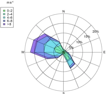
Figure 2. Distribution of the wind directions and wind speeds throughout the experimental period (December 2012–June 2013), as recorded by the meteorological station.
The wind speed value recorded during the experimental period by the meteorological station was 4 m s−1on average. The averaged wind speed value recorded by the meteorolog-ical station was very close to those recorded by the sonic anemometers installed on the flux stations within fields A, B, and C, with differences lower than 0.4 m s−1. The spatial homogeneity for wind speed was also observed in previous studies conducted at different locations within the same wa-tershed (Zitouna-Chebbi, 2009; Zitouna-Chebbi et al., 2012, 2015).
The wind rose obtained from the data collected at the meteorological station depicted two prevailing directions (Fig. 2). The first direction corresponded to winds coming from the south (directions between 70 and 220◦, clockwise; north is 0◦). The second direction corresponded to winds coming from the other directions, hereafter referred to as northwest winds. The topography induced downslope winds on field A and upslope winds on field B under northwest winds. The reverse was observed under south winds.
Micrometeorological conditions were analyzed using the atmospheric stability parameter ξ = (z − D)/LMO, where z is
measurement height (in meters), D is displacement height (in meters), and LMOis Monin–Obukhov length (in meters).
D was set as two-thirds of vegetation height, the latter be-ing derived from in situ measurements (see Sect. 2.6.2). The atmospheric stability parameter ξ was negative most of the time, with few values larger than 0.1, mainly during sun-rise or sunset. The ξ median values were −0.007, −0.011, and −0.010 for field A, B, and C, respectively. These val-ues corresponded to conditions of forced convection (neutral-ity or low instabil(neutral-ity) induced by large wind speeds. We did
not observe notable differences between northwest and south winds. Zitouna-Chebbi et al. (2012, 2015) obtained similar results with a dataset collected between 2003 and 2006 on different fields within the same study area.
Overall, the analysis of wind direction and micrometeo-rological conditions indicated that the wind regime did not stem from valley wind or land–sea breeze. Indeed, the wind direction did not depict any diurnal course in relation to an-abatic or katan-abatic flows or to land–sea temperature differ-ence, while the ξ parameter did not correspond to conditions of atmospheric stability with free convection.
2.6.2 Vegetation conditions
Throughout the experiment, the evolution of the wheat phe-nology was monitored using the so-called “BBCH scale im-proved” of Feekes and Large (Lancashire et al., 1991). Fields A, B, and C depicted similar phenological evolutions. The beginning of the tillering stage appeared on 15 January, and full tillering occurred on 19 February. The start of bolting was on 5 March, and full flowering was on 22 April. The seed maturity stage lasted from the beginning to the end of May, and the beginning of senescence was late May.
Vegetation height was measured on a weekly basis us-ing a tape measure. For each date, 30 height measurements were performed within each field, and were then averaged at the field scale. Vegetation height reached its maximum on 22 April, and maximum averaged values were 1.00, 0.87, and 0.98 m, for fields A, B, and C, respectively. Vegetation height measurements were next interpolated on a daily basis by us-ing a logistic function.
The vegetation height data indicated that the sonic anemometers and KH20 krypton hygrometers, set up around 2 m above soil surface, were located above the roughness sublayer. Indeed, the experimental conditions were typified by neutral or slightly unstable conditions that corresponded to a roughness sublayer extension from the ground up to 1.43 × vegetation height (Pattey et al., 2006).
Leaf area index of green leaves (GAI) was measured us-ing a planimeter. Every 2 weeks, all leaves were collected within three 1 m long transects to derive a spatially averaged value. GAI reached its maximum on 11 April, and maximum values were 2.5, 2.3, and 2.3 m2m−2for fields A, B, and C, respectively.
2.7 The dataset to be filled
Missing LE data stemmed from (1) total shutdowns of flux stations following battery discharges or vandalism acts, (2) malfunctions of KH20 krypton hygrometers after precip-itation events when air humidity permeated the sensor be-cause of seal degradation, and (3) rejection of LE data iden-tified as class V data by ST and ITC tests (Sect. 2.5.3).
Table 3 displays the number of available data derived from EC measurements over the three fields, when considering
Table 3. Summary of the available latent heat flux (LE) data derived from the eddy covariance measurements conducted on each of the three fields: dates of the beginning and ending of measurement periods, number of total daytime data over 30 min intervals for calculating the fluxes, numbers and percentages of data belonging to quality control classes (I–IV: good quality data; V: rejected data), numbers and percentages of the missing data due to dysfunctions of the KH20 sensors, and numbers and percentages of missing flux data due to total shutdowns of the flux stations.
Number of
Beginning End daytime 30 min KH20 System Field date date interval data I–IV (%) V ( %) dysfunctions (%) failure (%) A 6 Dec 2012 11 Jun 2013 4108 1685 (41) 162 (4) 1529 (37) 732 (18) B 11 Dec 2012 11 Jun 2013 4007 820 (21) 95 (2) 2965 (74) 127 (3) C 3 Jan 2013 11 Jun 2013 3603 2198 (61) 86 (2) 616 (17) 703 (20)
LE. It gives the beginning and end dates of the EC measure-ments, the number of daytime data over 30 min intervals, the numbers and proportions of data with good (classes I to IV) and bad quality (class V) according to ST and ITC tests, the number of missing data due to malfunctions of the Krypton hygrometer (KH20), and the number of missing data because of total shutdown of flux stations.
The ratio of filtered to original data ranged between 20 and 61 %. It was rather low compared to the ratios reported by former studies at the yearly timescale for worldwide flux networks such as FLUXNET (65 %), in which these ratios stemmed from system failures or data rejection (Baldocchi et al., 2000; Falge et al., 2001a, b). The low ratio we obtained in the current study was ascribed to KH20 malfunctions and to-tal shutdown of flux stations. Furthermore, the KH20 sensor installed on field B was out of order from the end of March until the end of the experiment because of severe instrumen-tal malfunctions.
The proportion of bad-quality data was low, with around 3 % of data belonging to class V. The results of the quality control tests did not exhibit any difference among the fields. For H , the percentages of data belonging to the high-quality classes (I to IV) were 85, 84, and 88 % for fields A, B, and C, respectively.
On the one hand, the rate of missing data for the current study, between 40 and 80 %, was much larger than that re-ported in former studies, i.e., between 25 and 35 % (Baldoc-chi et al., 2001; Falge et al., 2001a; Law et al., 2002). On the other hand, the rate of data rejected by quality control, between 2 and 4 %, was much lower for the current study compared to that reported in former studies, i.e., between 20 and 60 % (Papale et al., 2006). Therefore, the overall rate of data to be filled was comparable to that reported in former studies.
3 Methods
3.1 Rationale in choosing and implementing gap-filling methods
Amongst the existing LE gap-filling methods listed in the In-troduction (Table 1), we selected some methods that differ in the use of ancillary information, either meteorological vari-ables or energy fluxes. The meteorological data to be used were those provided by the meteorological station, while the flux data to be used were those collected at each of the three flux stations of interest (Sect. 2.3). We did not select meth-ods that involve measurements of soil water content or veg-etation canopy since energy fluxes indirectly account for the latter at a spatial scale closer to that of the LE missing data (see results about footprint analysis in the last paragraph of Sect. 2.5.3).
Amongst the existing LE gap-filling methods listed in the Introduction (Table 1), we selected the commonly used REd-dyProc method that relies on lookup tables (LUTs) and mean diurnal variation (MDV) to fill missing flux data with those collected under similar meteorological conditions or with av-eraged values over adjacent days. We also selected methods that fill LE gaps by using multilinear regressions on other energy flux data (Rn, H , and G). We did not select methods based on artificial neural networks because ensuring the rel-evance of calibration, testing, and validation steps requires large datasets of at least 1 year (Abudu et al., 2010; Beringer et al., 2007; Eamus et al., 2013; Papale and Valentini, 2003).
3.1.1 REddyProc
For the REddyProc method, we selected the online tool available at https://www.bgc-jena.mpg.de/bgi/index. php/Services/REddyProcWebRPackage (last access: 1 April 2018), and that is based on Reichstein et al. (2005). The REd-dyProc method combines the covariation of the convective fluxes with meteorological variables (Falge et al., 2001b) and the temporal autocorrelation of the convective fluxes (Reich-stein et al., 2005). Gaps are filled in accordance with avail-able information by considering three cases: (1) solar
radi-ation (Rg), air temperature (Tair), and vapor pressure deficit
(VPD) data are available; (2) Rg data only are available; and (3) none of the Rg, Tair, and VPD data are available.
For Case (1), the missing LE value is replaced by the av-erage value under similar meteorological conditions within a time window of ±7 days. Similar meteorological conditions correspond to Rg, Tair, and VPD values that do not deviate
by more than 50 W m−2, 2.5◦C, and 5 hPa, respectively. If no similar meteorological conditions occur within the ±7-day time window, the latter is extended to ±14 ±7-days.
For Case (2), a similar approach is taken. Similar meteo-rological conditions correspond to Rg deviation by less than 50 W m−2, and the window size is not extended.
For Case (3), the missing value is replaced by an adjacent value within ±1 h, or by an averaged value at the same time of the day that is derived from the mean diurnal course over ±1 day.
In case the three steps do not permit filling the gaps, the whole procedure is repeated while increasing the window sizes until the value can be filled. Thus, the window size in-creases using 7-day steps until ±70 days for Cases 1 and 2, and until ±140 days for Case 3, which obviously results in a degradation of the quality indicator.
3.1.2 LE reconstructed from Rn
Initially proposed by Cleverly et al. (2002), this method was successfully tested on our study site by Zitouna-Chebbi (2009). It assumes the stability of the LE / Rn ratio over a given period that can be 1 day, 1 month, or 1 year (Table 1). We implemented the method by first calibrating the linear regression LE = a Rn + b on existing LE and Rn data, and next applying the regression to missing LE data for which Rn was actually measured. This method will be re-ferred to as “LE–Rn method” hereafter.
3.1.3 LE reconstructed from multi-linear regression against other energy fluxes
This method is an extension of the LE–Rn method since LE is estimated as a linear combination of the other energy fluxes Rn, H , and G. As for the LE–Rn method, the multi-linear regression (MLR) method was implemented by first calibrat-ing the multi-linear regression on existcalibrat-ing LE, Rn, H , and G data (LE = a0Rn + b0G + c0H + d0), and next applying the regression to missing LE data for which the three other fluxes were actually measured. This method will be referred to as the “MLR method” hereafter.
Energy balance theoretically implies a0=1, b0= −1, c0= −1, and d0=0. However, this is not the case in prac-tice because of the energy imbalance problem for EC mea-surements. This problem has been mentioned in the liter-ature for vegetated canopies and bare soils, as well as for flat, mountainous, and hilly terrains (Foken, 2008; Ham-merle et al., 2007; Leuning et al., 2012; Wilson et al., 2002;
Zitouna-Chebbi et al., 2012, 2015). As reported by Leun-ing et al. (2012), the energy imbalance problem is that the sum of the convective flux (H + LE) underestimates avail-able energy (Rn − G) because of theoretical assumptions (e.g., neglecting storage terms or lateral turbulent transfers) and because of experimental assumptions (e.g., neglecting measurement inaccuracies, neglecting differences in mea-surement spatial extensions). Thus, applying the energy bal-ance equation LE = Rn− G − H would transfer energy im-balance onto LE estimates, which is not the case with the MLR method that involves a regression calibration (a06=1, b06= −1, c06= −1 and d06=0).
3.1.4 LE reconstructed from evaporative fraction
Evaporative fraction (EF) is defined as the ratio of LE over available energy (Rn − G) when assuming the latter equals the sum of convective fluxes (H + LE). Li et al. (2008) and Shuttleworth et al. (1989) showed that EF was almost con-stant during daytime hours. Although rebutted (Hoedjes et al., 2008; Van Niel et al., 2011), various studies stated that EF at midday (EFmd)is statistically representative of daily EF,
and thus recommended using EFmdfor estimating LE (Crago
and Brutsaert, 1996; Crago, 1996; Gentine et al., 2011; Li et al., 2008; Peng et al., 2013).
The estimation of missing LE data was twofold. In a first step, EFmdwas calculated on a daily basis by using the
mea-sured data over the 4 h centered on solar noon, provided that at least 75 % of the eight 30 min data were available between noon −2 h and noon +2 h for LE, Rn, and G.
EFmd= noon+2 h X noon-2 h LEi ,noon+2 h X noon-2 h (Rni−Gi) (1)
In a second step, the missing LE data were estimated as LE = (Rn− G) EFmd, when Rn and G were actually
mea-sured. This method will be referred to as the “EF method” hereafter.
Compared to the MLR method that implicitly accounts for the energy imbalance problem via the regression calibration, the EF method induced an overestimation of the convective fluxes by replacing H + LE with available energy Rn− G. Conversely, averaging EF around solar noon rather than over the diurnal course might induce an underestimation of EF at the daily timescale. Therefore, the EF method was likely to (1) induce some errors on LE estimates used for filling gaps and (2) increase energy imbalance for the reconstructed data because of the difference between H + LE and Rn − G.
3.2 Tailoring the gap-filling methods to the conditions of hilly crop fields
The gap-filling methods were tailored to the conditions of hilly crop fields by splitting the dataset on the basis of the airflow inclination that is driven by the combined effect of
Table 4. Splitting of the dataset into three periods when implementing the LE–Rn and MLR gap-filling methods. The three periods are labeled green vegetation (GV), pre-senescent vegetation (PS), and senescent vegetation (SV). They are indicated along with the vegetation and climatic conditions. GAI stands for leaf area index of green leaves; ET0stands for the reference evapotranspiration. Minimum and maximum GAI values are averaged values over the three fields A, B, and C. Cumulative precipitation, mean ET0, and mean air temperature are derived from measurements at the meteorological station.
Main Cumulative Mean Mean air Period Dates phenological GAI min GAI max precipitation ET0 temperature stage (m2m−2) (m2m−2) (mm) (mm day−1) (◦C) 6 Dec 2012 Seeding to
GV to beginning of 0.07 2.37 357.5 2.6 11.4 6 May 2013 dough stage
6 May 2013 Beginning of
PS to dough stage to 0.07 0.14 5 5.0 15.7 28 May 2013 fully ripened grain
28 May 2013 Fully ripened
SV to grain to – – 1 5.6 18.2
11 Jun 2013 senescence
wind direction, topography, and vegetation height. The anal-ysis of the experimental conditions showed that the wind regimes were typified by two main wind directions, i.e., northwest and south, which induces upslope and downslope winds on fields A and B (Sect. 2.6.1). Therefore, any of the three datasets for fields A, B, and C were split into two sub-datasets that correspond to northwest and south winds. We recall that (1) northwest winds correspond to downslope and upslope winds on fields A and B, respectively; (2) south winds correspond to upslope and downslope winds on fields A and B, respectively; and (3) field C was horizontal.
Most existing gap-filling methods for LE measurements include a prior splitting of the time series to be filled (Ta-ble 1), so that missing data are filled with existing observa-tions collected under similar condiobserva-tions. REddyProc relies on time windows up to 280 days, and the EF method relies on a daily time window. For both the LE–Rn and MLR meth-ods that assume stable regressions among energy fluxes, we split the dataset into three periods that differed in vegetation phenology. This accounted for changes in soil water content and vegetation height at monthly to seasonal timescales. The beginning and end of each period are given in Table 4, along with the vegetation and climatic conditions. The first period corresponded to active green vegetation, with moderate ref-erence evapotranspiration, and with abundant and frequent precipitation events that supply plant transpiration and soil evaporation. It was typified by the absence of water stress, and therefore large values for both EF and the LE / Rn ra-tio. We labeled this first period “GV” for green vegetation. The second period preceded grain maturation and leaf senes-cence. It corresponded to the beginning of water stress that resulted from the combined effect of limited precipitation and large reference evapotranspiration. We labeled this sec-ond period “PS” for pre-senescent vegetation. The third
pe-riod corresponded to leaf senescence and grain maturation. It corresponded to a pronounced water stress that resulted from the combined effect of no precipitation and large ref-erence evapotranspiration. We labeled this third period “SV” for senescent vegetation.
3.3 Assessing the performances of the gap-filling methods
The performances of the three gap-filling methods were as-sessed on filling rate, retrieval accuracy, and quality of gap-filled time series through energy balance closure. In order to make the performances of the four methods comparable, we used the following procedure.
Conversely to REddyProc, the LE–Rn, MLR, and EF methods were not able to fill gaps induced by total shutdowns of the flux stations. Therefore, we addressed the filling of the gaps that resulted from malfunctions of the KH20 sensors and quality filtering only.
For field B, the LE–Rn, MLR, and EF methods were not able to fill gaps induced by the shutdown of the KH20 sen-sor from the end of March (middle of the GV period) to the end of the experiment. Indeed, the EF method required Rn, G, and LE data on a daily basis, while the LE–Rn and MLR methods required data for each of the periods GV, PS, and SV, which excluded periods PS and SV. Therefore, we disre-garded the time period in question (from the end of March to the end of the experiment) for field B.
The filling performances were given in accordance with the number of reconstructible data (LE missing data because of both KH20 malfunctions and quality filtering). They were expressed as the ratio of reconstructed to reconstructible data.
The prior splitting of the time series to be filled is a com-mon procedure for most gap-filling methods (Table 1), but it is different from one method to another (Sect. 3.2). There-fore, we did not assess the performances of the gap-filling methods on the basis of the time periods GV, PS, and SV. We discriminated the periods GV, PS, and SV for the regression calibrations only (LE–Rn and MLR methods).
To quantify retrieval accuracy, REddyProc provides esti-mates for each existing datum, where the estimate is derived independently of the corresponding data. Therefore, we im-plemented a leave-one-out cross-validation (LOOCV) proce-dure to evaluate the retrieval accuracy for the LE–Rn, MLR, and EF methods. For this, any estimate for retrieval accu-racy was calculated by removing the corresponding reference value.
We evaluated the performances of the gap-filling methods before and after splitting the time series on the basis of wind direction (northwest or south). We separately considered the fields A, B, and C, where fields A and B are located on two opposite hillsides with upslope and downslope winds, and field C is located on a horizontal terrain.
The retrieval accuracy was quantified using absolute and relative root-mean-square error (RMSE and RRMSE) as well as mean absolute difference (MAE) and bias and coefficient of determination R2(Jacob et al., 2002; Moffat et al., 2007). To evaluate the quality of the gap-filled time series, we compared the sum of the convective energy fluxes (H + LE) against available energy (Rn − G) before and after gap fill-ing, where gap filling was conducted after splitting the time series on the basis of wind direction. Although energy bal-ance closure analysis is questionable for assessing the con-sistency of flux measurements, it permits the comparison of independent measurements.
4 Results
4.1 Filling performances of the gap-filling methods
For the three fields (A, B, C) and the two wind directions (northwest, south), Table 5 displays the number of recon-structible data (LE missing data because of KH20 malfunc-tions or LE data belonging to quality class V), as well as the number and percentage of reconstructed data by the four methods (REddyProc, LE–Rn, MLR, and EF). For each field, the total number of reconstructible data is also indicated, as well as the total number and corresponding percentage of re-constructed data. The total number of reconstructible data in Table 5 corresponds to that given in Table 3 (i.e., sum of LE missing data because of KH20 malfunctions and of LE data belonging to quality class V), apart from field B (2083 ver-sus 3060) for which we restricted the time period to the GV period since no LE data were available on periods PS and SV because of the KH20 shutdown (second item in Sect. 3.3).
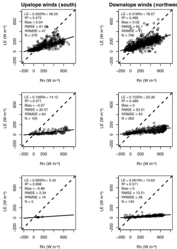
Figure 3. Calibration of the LE–Rn gap-filling method on field A. Columns 1 and 2 correspond to upslope and downslope winds, re-spectively. Lines 1, 2, and 3 correspond to the three periods (GV, PS, SV) that differed in vegetation phenology, soil water content, and climatic conditions. The dashed line is the 1 : 1 line, and the continuous line is the regression line. R2is the coefficient of deter-mination. RMSE and RRMSE are absolute and relative root-mean-square errors, respectively. N is the number of flux data calculated over 30 min intervals.
With both the REddyProc and LE–Rn methods, all the missing LE data could be reconstructed. The MLR method permitted the reconstruction of 84, 86, and 90 % of the miss-ing LE data, on fields A, B, and C respectively. The EF method permitted the reconstruction of 32, 19, and 70 % of the missing LE data, on fields A, B, and C, respectively. The reconstruction rates obtained with the MLR method were similar on fields A, B and C. Conversely, the reconstruction rate with the EF method was much larger on field C (flat ter-rain) than that on fields A and B (sloping terrains). Overall, the filling rate was the same for a given field, whether we split the time series on the basis of wind direction or not.
4.2 Accuracy of the gap-filling methods
The calibration of the LE–Rn method for the three periods (GV, PS, and SV) was similar for fields A (Fig. 3), B, and C
Table 5. Filling rate performance for each of the four gap-filling methods (REddyProc, LE–Rn, MLR, EF), expressed as the number and percentage of reconstructible LE data that were actually reconstructed. The filling rates are given for each field (A, B, C) and each wind direction. S and NW stand for south and northwest winds, respectively. Up and down stand for upslope and downslope winds, respectively, for the sloping fields A and B (field C was flat).
Field A Field B Field C Field A Field B Field C All data All data All data S (up) NW (down) Total S (down) NW (up) Total S NW Total Number of reconstructible 1691 2083 702 585 1106 1691 716 1367 2083 230 472 702 data REddyProc 1691 2083 702 585 1106 1691 716 1367 2083 230 472 702 (100) (100) (100) (100) (100) (100) (100) (100) (100) (100) (100) (100) Number of LE–Rn 1691 2083 702 585 1106 1691 716 1367 2083 230 472 702 reconstructed (100) (100) (100) (100) (100) (100) (100) (100) (100) (100) (100) (100) data (%) MLR 1415 1789 631 489 926 1415 626 1163 1789 199 432 631 (84) (86) (90) (84) (84) (84) (87) (85) (86) (87) (92) (90) EF 534 398 494 226 308 534 123 275 398 156 338 494 (32) (19) (70) (39) (28) (32) (17) (20) (19) (68) (72) (70)
(Fig. S1a and b in the Supplement). The LE / Rn ratio exhib-ited a notable temporal stability for each of the three periods, and we did not observe any distinct scatter for the period GV, even if the scattering was larger compared to the periods PS and SV. However, we observed significant differences in slope and offset from one period to another, with changes in slope between 90 and 170 % (relative to mean value), and changes in offset between 60 and 120 % (relative to mean value).
We obtained similar LE–Rn regressions for fields A (Fig. 3) and B (Fig. S1a) when splitting the time series on the basis of south and northwest winds that correspond to up-slope (respectively downup-slope) and downup-slope (respectively upslope) winds on field A (respectively B). Apart from the SV period with too few data on field A, we noted some dif-ferences in regressions between the two wind directions for any period, with changes in slope between 5 and 50 % (rel-ative to mean value) and changes in offset between 40 and 80 % (relative to mean value). Conversely, the differences were lower on field C with a flat terrain (see Fig. S1b), with changes in slope between 0.5 and 10 % (relative to mean value) and changes in offset between 15 and 30 % (relative to mean value). A covariance analysis conducted on the re-gression coefficients showed that the changes in slope and offset were statistically significant in most cases (Table S1).
We quantified the retrieval accuracies of the four gap-filling methods by comparing reference data and gap-gap-filling retrievals of LE over 30 min intervals for each field and each wind direction (Fig. 5 and Table S2). The retrieval accuracies were obtained using a LOOCV procedure (Sect. 3.3). We ob-served the following trends.
The four methods provided similar retrieval accuracies, with differences among RMSE values lower than 20 W m−2. Bias values were almost null, apart from the EF method. To a lesser extent, the RMSE values were lower with
REd-dyProc, which also provided better R2 values, and the EF method provided the larger RMSE and bias values, down to −20 W m−2for bias.
Regardless of the gap-filling method, the retrieval accura-cies were similar for fields A and C, whereas they were lower for field B.
The method performances could be either different or sim-ilar before and after the splitting of the time series on the ba-sis of wind direction. For field A, the RMSE values were sim-ilar for upslope and downslope winds, and they were compa-rable to those obtained before the splitting. For field B, the RMSE values were much lower (respectively slightly larger) for downslope winds (respectively upslope winds) compared to those obtained before splitting the time series. For field C with a flat terrain, the statistical indicators were comparable before and after the splitting.
4.3 Energy balance closure analysis
We recall that the gap-filling retrievals we considered for en-ergy balance closure analysis were those obtained by split-ting the time series on the basis of wind direction (Sect. 3.3). We obtained similar results for energy balance closure for field A (Fig. 4) and fields B and C (Fig. S2a and b). Before and after gap filling, the sum of the convective fluxes system-atically underestimated available energy, apart from field B after gap filling with the EF method. On a field basis, change in energy balance closure from one gap-filling method to an-other was 15 % for field A, 65 % for field B, and 44 % for field C, according to changes in the H + LE versus Rn − G regression slope. On a method basis, energy balance closure varied from 5 % (MLR) to 32 % (EF) from one field to an-other, according to changes in the H + LE versus Rn − G regression slopes. Finally, energy balance closure could be better after gap filling, and energy balance closure on
slop-● ●
Figure 4. Energy balance (EB) closure for field A. Flux data are calculated over 30 min intervals. Statistical indicators correspond to the comparison of convective energy (H + LE) on the y axis against the available energy (Rn − G) on the x axis, before (top left subplot) and after (other subplots) reconstruction of LE data by the four gap-filling methods. The dashed line is the 1 : 1 line, and the continuous line is the regression line. Letters a and b are the slope and the in-tercept of the linear regression, respectively. R2is the coefficient of determination. MAE is the mean absolute error. RMSE and RRMSE are absolute and relative root-mean-square errors, respectively. N is the number of 30 min interval data.
ing fields A and B was comparable to that on the flat field C.
When comparing energy balance closure after gap filling with the four methods, we could not identify any clear trend on the basis of the (H + LE) versus (Rn − G) linear regres-sion. Gap filling with the LE–Rn method provided among the best energy balance closure, and gap filling with the REd-dyProc method provided among the worst energy balance closures. Energy balance closure was very similar for the LE–Rn and MLR methods, with changes in the regression
REP LE−Rn MLR EF 0 20 40 60 80 Field A R M S E ( W m - ²) All NW S REP LE−Rn MLR EF 0 20 40 60 80 Field B REP LE−Rn MLR EF 0 20 40 60 80 Field C REP LE−Rn MLR EF −15 −10 −5 0 B ia s ( W m - ²) REP LE−Rn MLR EF −15 −10 −5 0 REP LE−Rn MLR EF −15 −10 −5 0 REP LE−Rn MLR EF 0.0 0.2 0.4 0.6 0.8 R² REP LE−Rn MLR EF 0.0 0.2 0.4 0.6 0.8 REP LE−Rn MLR EF 0.0 0.2 0.4 0.6 0.8
Figure 5. Accuracy of LE retrievals for the four gap-filling methods (REddyProc labeled as REP, LE–Rn, MLR, EF). Fluxes were cal-culated over 30 min intervals. Retrieval accuracy is given for each field (A, B, C) and each wind direction (All stands for all data. NW and S stand for northwest and south winds, respectively). Accuracy is quantified using statistical indicators (absolute RMSE, bias, co-efficient of determination R2).
slope between 2.5 % (field C) and 4.5 % (field A). Further, the EF method could provide the worst (field A) or the best (field B) energy balance closure. The scattering around the (H + LE) versus (Rn − G) regressions was reduced after gap filling, either slightly with the REddyProc and EF methods, or a lot with the LE–Rn and MLR methods.
5 Discussion
5.1 Filling performances of the gap-filling methods
The filling rate was maximal with the REddyProc and LE– Rn methods. Indeed, REddyProc relies on existing LE values within a given time window, either corresponding to simi-lar meteorological variables or derived from averaged diur-nal courses. Similarly, the LE–Rn method relied on
contin-uous measurements of Rn. The MLR method was less effi-cient than the REddyProc and LE–Rn methods because of both missing H measurements and H data rejection by qual-ity control. In this case, the filling rate was comparable to the percentage of available H data given in Sect. 2.7 (84, 86 and 90 % versus 85, 84, and 88 % for fields A, B, and C, re-spectively). The worst efficiency of the EF-based gap-filling method was explained by the fact that Rn, G, and LE data around solar noon are required on a daily basis.
The filling rate was similar whether we split the time se-ries on the basis of wind direction or not. For REddyProc, this was explained by the capability of the method to find LE data under similar meteorological conditions or to obtain averaged values from diurnal courses within a scalable time window. For the LE–Rn and the MLR methods, this was ex-plained by existing data for regressions within the three pe-riods GV, PS, and SV, when applicable. For the EF method, this was explained by the daily basis computation of EF and the subsequent filling at the daily timescale. Overall, the four methods were able to fill all gaps in the time series, in spite of larger gap occurrences induced by the splitting of the time series on the basis of wind direction. Also, it is important to note that conversely to the LE–Rn, MLR, and EF meth-ods that relied on energy fluxes (Rn, G, and H ), REddyProc had the capability of filling gaps induced by total shutdowns of the flux stations, although we did not address these to-tal shutdowns to make the performances of the four methods comparable.
We could not compare the filling rates we obtained in the current study against outcomes from the former studies listed in Table 1 for LE data owing to the absence of information on this issue.
5.2 Accuracy of the gap-filling methods
When calibrating the LE–Rn method, it was relevant to split the time series into the three periods GV, PS, and SV because of large changes in the LE–Rn regression from one period to another. The strong decrease in LE / Rn ratio from GV to SV was ascribed to the decrease in LE magnitude because of vegetation senescence that was combined with no pre-cipitation and increasing reference evapotranspiration. This emphasizes the impact of changes in soil water content and vegetation canopy at monthly to seasonal timescales. When calibrating the LE–Rn method, it was also relevant to split the time series on the basis of northwest and south winds. Indeed, some differences were observed between the two wind direc-tions for the periods GV and PS, and these differences were larger for sloping terrains (fields A and B) than for the flat ter-rain (field C). Compared to former studies listed in Table 1, these outcomes were consistent with those from Zitouna-Chebbi (2009). Indeed, the latter reported the need to split time series into distinct periods and wind directions, so that it was possible to take into account changes in aerodynamic
conditions for measurements collected within the same study area, over other crop fields, and during other years.
The slightly better accuracies obtained with REddyProc indicates that this method was able to find appropriate LE values under similar meteorological conditions within a given time window, in spite of possible changes in soil water content. LE–Rn and MLR provided very similar accuracies. We expected that MLR would outperform LE–Rn because of the additional inclusion into the regression of G and H fluxes that are driven by vegetation canopy and soil water content. Then, the similar accuracies might result from too large time windows for periods GV, PS, and SV, and espe-cially for period GV with large scattering around the regres-sion line (see for instance Fig. 3 with the LE–Rn regresregres-sion). The EF method provided lower accuracies. We expected bet-ter accuracies with the EF method that filled gaps on a daily basis, and the underperformance might result from the com-bination of (1) the EF underestimation at the daily timescale when computed between 10:00 and 14:00 solar time, and (2) the overestimation of H + LE by Rn − G as a result of energy imbalance. Overall, the method performances were driven by the temporal dynamics of the local conditions in terms of micrometeorology, vegetation canopy, and soil wa-ter content. For instance, large precipitations were likely to induce sharp changes in soil water content, thus giving the EF method an advantage that is based on a daily basis com-putation, and giving the REddyProc method a disadvantage that relies on similar meteorological conditions or average diurnal courses.
Overall, the RMSE values between reference data and gap-filling retrievals of LE ranged between 20 and 90 W m−2, and almost two-thirds of these values were lower than 50 W m−2. The retrieval accuracy was similar for the four gap-filling methods, and it was comparable to those reported by the previous studies listed in Table 1 (e.g., between 25 and 50 W m−2for RMSE).
Finally, the performances could be better when splitting the time series on the basis of northwest and south winds, with much lower RMSE values for downslope winds. This was not systematic for the sloping fields, but was system-atic for all methods when applicable, although these methods involved different information for the reconstruction of the missing data. Thus, our study confirmed that it may be nec-essary to discriminate upslope and downslope winds when implementing gap-filling methods. This is consistent with re-ports from Zitouna-Chebbi et al. (2012, 2015), who showed the need to discriminate upslope and downslope winds when correcting the influence of airflow inclination on EC mea-surements collected over hilly crop fields.
5.3 Energy balance closure analysis
For the LE–Rn and MLR methods, energy balance closures were similar, they varied little from one field to another, and they were better than those obtained with the REddyProc
and EF methods. This was ascribed to the constraint on en-ergy balance closure when replacing gaps with LE estimates derived from regression between energy balance fluxes (LE versus Rn on the one hand, and LE versus Rn, G, and H on the other hand). Energy balance closure was worse with REddyProc, and it varied much from one field to another. This was ascribed to the lack of constraint on energy bal-ance closure when replacing gaps with LE data collected at different times. For EF, energy balance closure varied much from one field to another, and especially on field B with (H + LE) overestimating (Rn − G). This might be explained by changes in compensation effects between (1) the EF un-derestimation at the daily timescale when computed between 10:00 and 14:00 solar time and (2) the overestimation of H +LE by Rn − G as a result of energy imbalance.
For the four gap-filling methods, energy balance closure after reconstruction of the LE data was comparable to that observed before gap filling, which showed the consistency of the gap-filled time series. Further, energy balance closure for the two sloping fields (A and B) was comparable to that ob-tained on the flat field (C), which showed the consistency of the reconstructed data after the splitting of the time series on the basis of upslope–downslope winds. We could not com-pare the energy balance closures we obtained in the current study against the outcomes from the former studies listed in Table 1 for LE data owing to the absence of information on this issue. Nevertheless, our values of energy balance disclo-sure ([15–35 %]) were comparable to those reported in the literature ([10–30 %]) for flat, hilly, and mountainous terrains (Foken, 2008; Hammerle et al., 2007; Li et al., 2008; Wilson et al., 2002; Zitouna-Chebbi et al., 2012, 2015).
6 Conclusions
For the four gap-filling methods we evaluated (REddyProc, LE–Rn, MLR, and EF), the retrieval accuracies were sim-ilar and comparable to instrumental accuracies. The filling rate was maximal for REddyProc and LE–Rn, whereas it was lower for MLR and EF. Therefore, the REddyProc and LE– Rn methods were the most appropriate for our study case, in terms of completing time series as much as possible while providing retrievals with good quality. This outcome applied even more for the REddyProc method that is able to fill gaps induced by total shutdowns, although a deeper analy-sis is needed beforehand to evaluate the retrieval accuracies in such situations.
Our results led us to recommend the splitting of LE time series on the basis of wind direction, prior to the implemen-tation of the gap-filling methods. Indeed, the prior splitting of time series on the basis of wind direction might improve retrieval accuracies, although the benefit was not systematic. In addition, the obtained accuracies on LE estimates after gap filling were comparable to those reported in the literature for flat and mountainous areas, and the same applied for energy
balance closure as a consistency indicator for the filled time series. Finally, the splitting of the time series did not impact the gap-filling rate, in spite of larger gap occurrences. There-fore, we conclude that it is possible to conduct gap filling for time series collected over hilly terrains, provided the prior splitting of the time series is applied in an appropriate man-ner by discriminating upslope and downslope winds.
Our study case is widespread within the Mediterranean basin because of orography and climate conditions within coastal areas across the Mediterranean shores. To a lesser ex-tent, the outcomes of our studies are also of potential inter-est for hilly watersheds in eastern Africa, India, and China. Conversely, the experiment on which the current study re-lied lasted over one crop growth cycle only, and we off-set this temporal restriction by simultaneously considering three locations that differed much in topographical condi-tions and resulting airflow inclination. Nevertheless, future works should strengthen the outcomes of the current study by addressing (1) a larger panel of environmental conditions in relation to climate, vegetation type, and water statuses and (2) consecutive vegetation growth cycles.
Data availability. The data used in this study are available accord-ing to the data policy of the Environmental Research Observatory OMERE (Molénat et al., 2018; http://www.umr-lisah.fr/omere, last access: 1 April 2018).
The Supplement related to this article is available online at https://doi.org/10.5194/gi-7-151-2018-supplement.
Competing interests. The authors declare that they have no conflict of interest.
Acknowledgements. This study was supported by the IRD JEAI JASMIN-Tunisia project (INRGREF, INAT, and LISAH), the IRD/ARTS program, the MISTRALS/SICMED project, the Agropolis Foundation (contract 0901-013), and the ANR TRANSMED ALMIRA project (contract ANR-12-TMED-0003-01). The ORE OMERE is thanked for providing the meteorological data. We also thank the International Joint Laboratory NAILA. We are extremely grateful to Tim McVicar and to the anonymous reviewers for constructive discussions that helped to improve the paper.
Edited by: Marina Díaz-Michelena Reviewed by: two anonymous referees
References
Abudu, S., Bawazir, A. S., and King, J. P.: Infilling Missing Daily Evapotranspiration Data Using Neural Networks, J. Irrig. Drain. Eng., 136, 317–325, 2010.
Alavi, N., Warland, J. S., and Berg, A. A.: Filling gaps in evapotran-spiration measurements for water budget studies: Evaluation of a Kalman filtering approach, Agr. Forest Meteorol., 141, 57–66, 2006.
Allen, R. G., Pereira, L. S., Raes, D., and Smith, M.: Crop evapotranspiration-Guidelines for computing crop water requirements-FAO Irrigation and drainage paper 56, FAO, Rome, 300, D05109, 1998.
Appels, W. M., Bogaart, P. W., and van der Zee, S. E. A. T. M.: Sur-face runoff in flat terrain: How field topography and runoff gen-erating processes control hydrological connectivity, J. Hydrol., 534, 493–504, 2016.
Aubinet, M., Grelle, A., Ibrom, A., Rannik, Ü., Moncrieff, J., Fo-ken, T., Kowalski, A.S., Martin, P.H., Berbigier, P., Bernhofer, C., Clement, R., Elbers, J., Granier, A., Grünwald, T., Morgen-stern, K., Pilegaard, K., Rebmann, C., Snijders, W., Valentini, R., and Vesala, T.: Estimates of the Annual Net Carbon and Wa-ter Exchange of Forests: The EUROFLUX Methodology, edited by: Fitter, A. H. and Raffaelli, D. G., Adv. Ecol. Res., 113–175, Academic Press, 1999.
Baldocchi, D., Finnigan, J., Wilson, K., Paw, U, K. T., and Falge, E.: On Measuring Net Ecosystem Carbon Exchange Over Tall Vege-tation on Complex Terrain, Bound.-Lay. Meteorol., 96, 257–291, 2000.
Baldocchi, D., Falge, E., Gu, L., Olson, R., Hollinger, D., Running, S., Anthoni, P., Bernhofer, C., Davis, K., Evans, R., Fuentes, J., Goldstein, A., Katul, G., Law, B., Lee, X., Malhi, Y., Meyers, T., Munger, W., Oechel, W., Paw, K. T., Pilegaard, K., Schmid, H. P., Valentini, R., Verma, S., Vesala, T., Wilson, K., and Wofsy, S.: FLUXNET: A New Tool to Study the Temporal and Spatial Variability of Ecosystem–Scale Carbon Dioxide, Water Vapor, and Energy Flux Densities, B. Am. Meteorol. Soc., 82, 2415– 2434, 2001.
Beringer, J., Hutley, L. B., Tapper, N. J., and Cernusak, L. A.: Sa-vanna fires and their impact on net ecosystem productivity in North Australia, Global Change Biol., 13, 990–1004, 2007. Blyth, E. M.: Estimating Potential Evaporation over a Hill,
Bound.-Layer Meteorol., 92, 185–193, 1999.
Chen, Y.-Y., Chu, C.-R., and Li, M.-H.: A gap-filling model for eddy covariance latent heat flux: Estimating evapotranspiration of a subtropical seasonal evergreen broad-leaved forest as an ex-ample, J. Hydrol., 468–469, 101–110, 2012.
Cleverly, J. R., Dahm, C. N., Thibault, J. R., Gilroy, D. J., and Allred Coonrod, J. E.: Seasonal estimates of actual evapo-transpiration from Tamarix ramosissima stands using three-dimensional eddy covariance, J. Arid Environ., 52, 181–197, 2002.
Crago, R. D.: Conservation and variability of the evaporative frac-tion during the daytime, J. Hydrol., 180, 173–194, 1996. Crago, R. and Brutsaert, W.: Daytime evaporation and the
self-preservation of the evaporative fraction and the Bowen ratio, J. Hydrol., 178, 241–255, 1996.
Dupont, S., Brunet, Y., and Finnigan, J. J.: Large-eddy simulation of turbulent flow over a forested hill: Validation and coherent structure identification, Q. J. Roy. Meteorol. Soc., 134, 1911– 1929, 2008.
Eamus, D., Cleverly, J., Boulain, N., Grant, N., Faux, R., and Villalobos-Vega, R.: Carbon and water fluxes in an arid-zone Acacia savanna woodland: An analyses of seasonal patterns and responses to rainfall events, Agr. Forest Meteorol., 182–183, 225–238, 2013.
Falge, E., Baldocchi, D., Olson, R., Anthoni, P., Aubinet, M., Bern-hofer, C., Burba, G., Ceulemans, R., Clement, R., Dolman, H., Granier, A., Gross, P., Grünwald, T., Hollinger, D., Jensen, N.-O., Katul, G., Keronen, P., Kowalski, A., Lai, C.T., Law, B.E., Meyers, T., Moncrieff, J., Moors, E., Munger, J. W., Pilegaard, K., Rannik, Ü., Rebmann, C., Suyker, A., Tenhunen, J., Tu, K., Verma, S., Vesala, T., Wilson, K., and Wofsy, S.: Gap filling strategies for defensible annual sums of net ecosystem exchange, Agr. Forest Meteorol., 107, 43–69, 2001a.
Falge, E., Baldocchi, D., Olson, R., Anthoni, P., Aubinet, M., Bern-hofer, C., Burba, G., Ceulemans, R., Clement, R., Dolman, H., Granier, A., Gross, P., Grünwald, T., Hollinger, D., Jensen, N.-O., Katul, G., Keronen, P., Kowalski, A., Ta Lai, C., Law, B. E., Meyers, T., Moncrieff, J., Moors, E., William Munger, J., Pile-gaard, K., Rannik, Ü., Rebmann, C., Suyker, A., Tenhunen, J., Tu, K., Verma, S., Vesala, T., Wilson, K., and Wofsy, S.: Gap filling strategies for long term energy flux data sets, Agr. Forest Meteorol., 107, 71–77, 2001b.
Foken, T.: The energy balance closure problem: an overview, Ecol. Appl., 18, 1351–1367, 2008.
Foken, T. and Wichura, B.: Tools for quality assessment of surface-based flux measurements, Agr. Forest Meteorol., 78, 83–105, 1996.
Foken, T., Göockede, M., Mauder, M., Mahrt, L., Amiro, B., and Munger, W.: Post-Field Data Quality Control, edited by: Lee, X., Massman, W., and Law, B., Handbook of Micrometeorology (181–208), Springer Netherlands, 2005.
Geissbühler, P., Siegwolf, R., and Eugster, W.: Eddy Covariance Measurements On Mountain Slopes: The Advantage Of Surface-Normal Sensor Orientation Over A Vertical Set-Up, Bound.-Lay. Meteorol., 96, 371–392, 2000.
Gentine, P., Entekhabi, D., and Polcher, J.: The Diurnal Behav-ior of Evaporative Fraction in the Soil–Vegetation–Atmospheric Boundary Layer Continuum, J. Hydrometeorol., 12, 1530–1546, 2011.
Goulden, M. L., Munger, J. W., Fan, S.-M., Daube, B. C., and Wofsy, S. C.: Measurements of carbon sequestration by long-term eddy covariance: methods and a critical evaluation of ac-curacy, Global Change Biol., 2, 169–182, 1996.
Greco, S. and Baldocchi, D. D.: Seasonal variations of CO2 and water vapour exchange rates over a temperate deciduous forest, Global Change Biol., 2, 183–197, 1996.
Grünwald, T. and Bernhofer, C.: Regression modelling used for data gap filling of carbon flux measurements, Forest Ecosyst. Modell., Upscal. Remote Sens., 61, 61–67, 1999.
Hammerle, A., Haslwanter, A., Schmitt, M., Bahn, M., Tappeiner, U., Cernusca, A., and Wohlfahrt, G.: Eddy covariance measure-ments of carbon dioxide, latent and sensible energy fluxes above a meadow on a mountain slope, Bound.-Lay. Meteorol., 122, 397–416, 2007.
Hiller, R., Zeeman, M., and Eugster, W.: Eddy-Covariance Flux Measurements in the Complex Terrain of an Alpine Valley in Switzerland, Bound.-Lay. Meteorol., 127, 449–467, 2008.