Using Unlabeled Data to Discover Bivariate Causality with Deep Restricted Boltzmann Machines

HAL Id: hal-01938646

https://hal.archives-ouvertes.fr/hal-01938646

Submitted on 28 Nov 2018

HAL is a multi-disciplinary open access

archive for the deposit and dissemination of

sci-entific research documents, whether they are

pub-lished or not. The documents may come from

teaching and research institutions in France or

abroad, or from public or private research centers.

L’archive ouverte pluridisciplinaire HAL, est

destinée au dépôt et à la diffusion de documents

scientifiques de niveau recherche, publiés ou non,

émanant des établissements d’enseignement et de

recherche français ou étrangers, des laboratoires

publics ou privés.

Using Unlabeled Data to Discover Bivariate Causality

with Deep Restricted Boltzmann Machines

Nataliya Sokolovska, Olga Permiakova, Sofia Forslund, Jean-Daniel Zucker

To cite this version:

Nataliya Sokolovska, Olga Permiakova, Sofia Forslund, Jean-Daniel Zucker. Using Unlabeled Data to

Discover Bivariate Causality with Deep Restricted Boltzmann Machines. IEEE/ACM Transactions

on Computational Biology and Bioinformatics, Institute of Electrical and Electronics Engineers, In

press, �10.1109/TCBB.2018.2879504�. �hal-01938646�

Using Unlabeled Data

to Discover Bivariate Causality

with Deep Restricted Boltzmann Machines

Nataliya Sokolovska, Olga Permiakova, Sofia K. Forslund, and Jean-Daniel Zucker

metabolism. The reconstruction of causal relations purely from non-temporal observational data is challenging. We address the problem of causal inference in a bivariate case, where the joint distribution of two variables is observed. We consider, in particular, data on discrete domains. The state-of-the-art causal inference methods for continuous data suffer from high computational complexity. Some modern approaches are not suitable for categorical data, and others need to estimate and fix multiple hyper-parameters. In this contribution, we introduce a novel method of causal inference which is based on the widely used assumption that ifXcausesY,

thenP (X)andP (Y |X)are independent. We propose to explore a semi-supervised approach whereP (Y |X)andP (X)are

estimated from labeled and unlabeled data respectively, whereas the marginal probability is estimated potentially from much more (cheap unlabeled) data than the conditional distribution.

We validate the proposed method on the standard cause-effect pairs. We illustrate by experiments on several benchmarks of biological network reconstruction that the proposed approach is very competitive in terms of computational time and accuracy compared to the state-of-the-art methods. Finally, we apply the proposed method to an original medical task where we study whether drugs confound human metagenome.

Index Terms—Causal inference, semi-supervised learning, probabilistic models, metagenomic data.

F

1

I

I

observational biological data in absence of time series or controlled perturbation is an important problem. In the past decades, the attention to the problem of causal inference has grown due to necessity to reveal causality in real life applications. In particular, in the medical domain, revealing causal relations from a data set can help to improve clinical diagnostics, and to increase the quality of treatment and medication.

Mechanism of action of many prescribed drugs remain unclear. Metformin is the most prescribed treatment for the type 2 diabetic patients, since it is relatively cheap, safe, and its important beneficial effects on blood glucose and cardiovascular parameters have been shown [1]. The main hypothesis of metformin action is that the drug mediates its antihyperglicemic effects by suppressing hepatic glucose output via the activation of AMP-activated protein kinase (AMPK) - dependent and AMPK - independent pathways in the liver [2]. However, recently some studies [3] confirmed hypotheses that metformin also acts through pathways in

• N. Sokolovska is with the Sorbonne University, NutriOmics team, IN-SERM, Paris, France

E-mail: nataliya.sokolovska@sorbonne-universite.fr

• O. Permiakova is with the University Grenoble Alpes, CEA,

BIG/BGE/EDyP, France

• S. K. Forslund is with the Experimental and Clinical Research Center, a cooperation of Charit´e-Universit¨atsmedizin Berlin and Max Delbruck Center for Molecular Medicine, 13125 Berlin, Germany; European Molec-ular Biology Laboratory, Structural and Computational Biology Unit, 69117 Heidelberg, Germany.

• J.-D. Zucker is with the UMMISCO, IRD, Bondy, France.

the gut.

In this paper, our goals are:

• to develop a robust causal inference method, since biological data are always limited and noisy,

• suspecting microbial mediation of therapeutic effects of metformin, test this hypothesis on a real data. Instead of learning causal structure of an entire dataset, some scientists focus on analysis of causal relations of two variables only. Modern conditional independence-based causal discovery methods (see, e.g., [4], [5] for general overview) construct Markov equivalent graphs, and these methods fail in the case of two variables, since X → Y and Y → X are Markov equivalent.

In this contribution, we focus on a family of causal inference methods which are based on a postulate telling that if X → Y , then the marginal distribution P (X) and the conditional distribution P (Y |X) are independent [6], [7], [8]. These approaches provide causal directions based on the estimated conditional and marginal distributions from observed non-temporal data. The bivariate methods are quite different from another state-of-art approach called 3off2 [9] where the algorithm needs three variables to infer a direction, since it considers all possible triplets in data, and looks for colliders in a graph. Therefore, the 3off2 is not suitable for bivariate cases. One of the most important problems in the causal inference in a bivariate case, is to estimate the conditional and the marginal probabilities from noisy limited observed data as accurate as possible.

Deep learning methods [10] are becoming the preferred approach for various applications in artificial intelligence

and machine learning, since they usually achieve the best accuracy. We are interested in particular in stochastic neu-ral networks, whose activation units have a probabilistic element. Such a choice is motivated by the fact that con-ditional and marginal probabilities P (Y |X) and P (X) can be estimated by a deep model. Deep restricted Boltzmann machines (DRBM) originally introduced by [11] is a deep stochastic model with one layer of visible units and several hidden units.

Our contribution is multifold:

• We introduce a novel semi-supervised method of inferring causal directions that allows to discover the associations between different pairs of factors.

• We propose to estimate the conditional and marginal probabilities which are the key elements to infer directions, using the deep RBM.

• We illustrate by our experiments on benchmark data that the proposed method is computationally effi-cient and its performance is highly competitive com-pared to the state-of-the-art methods. It outperforms the existing methods in terms of accuracy.

• We consider a real biomedical problem of revealing causality in rich original metagenomic data. The interest to infer causality in metagenomic data is to verify hypotheses that drugs effects on metabolism are microbially mediated. We show that the proposed approach is efficient on the real complex data, and discuss the obtained results.

The paper is organized as follows. Related work dis-cusses the state-of-art methods of the bivariate causal infer-ence. We consider continuous and discrete supervised and unsupervised methods for causal inference, and then we introduce a semi-superivsed pairwise probabilistic method. The deep restricted Boltzmann machines and the ways to compute the marginal and conditional probabilities are described before the numerical results. We discuss the results of our experiments on some standard challenges, benchmark networks, and on an original medical problem. Concluding remarks and perspectives close the paper.

2

R

W

There are two families of causal inference methods: Additive Noise Models (ANM) and Information Geometric Causal Inference (IGCI) [12].

Additive noise models (ANM) introduced by [13] and [14] is an attempt to determine causality between two vari-ables. The ANM assume that if there is a function f and some noise E such that Y = f (X) + E, where E and X are independent, then the direction is inferred to X → Y . A generalisation of the ANM, called post-nonlinear models, was introduced by [15]. However, the known drawback of the ANM is that the model is not always suitable for inference on categorical data [16].

Another research avenue exploiting the asymmetry be-tween cause and effect are the linear trace (LTr) method [17] and information-geometric causal inference (IGCI) [7]. They rely on an assumption that if X → Y , and generating P (X) is independent from P (Y |X), then the trace condition if fulfilled in the causal direction and violated in the opposite

one. The IGCI method exploits the fact that the density of the cause and the log slope of the function-transforming cause to effect are uncorrelated. At the same time, the density of the effect and the log slope of the inverse of the function are positively correlated.

Origo [18] is a causal discovery method based on the Kolmogorov complexity. The Minimum Description Length (MDL) principle can be used to approximate the Kol-mogorov complexity for real applications. Namely, from algorithmic information viewpoint, if X → Y , then the shortest program that computes Y from X will be more simple than the shortest program computing X from Y. However, the performance of Origo does not seem to be competitive compared to the ANM.

A number of recent, reported to be efficient causal discovery methods (see, e.g., [6], [7], [8]) are based on a postulate of independence of input and output, telling that a causal direction can be inferred from estimated marginal and conditional probabilities of random variables from a data set. In the following, we investigate this research direc-tion.

3

P

S

-S

C

I

-ENCE

In this section, we consider methods which rely on the following postulate [6], [7], [8] and assumptions.

Postulate 1. If X → Y , then the marginal distribution of the

cause P (X) and the conditional distribution of the effect given the cause P (Y |X) are ”independent” in the sense that P (Y |X) contains no information about P (X) and vice versa.

Assumption 1. We assume that the training procedure

has access to N pairs {Xi, Yi}Ni=1 of observations, and

N0 points of unlabeled data {Xi}N 0

i=1. Let us denote

X = (X1, . . . , XN) as a one-dimensional vector, and

Y = (Y1, . . . , YN) is also a vector of length N .

Assumption 2. Only X and Y are observed. We assume that

no confounders are present, no selection bias, and no feedback.

The Assumption 2 is strong, and it is often violated in real applications. If a confounder can be measured, the stan-dard solution is to adjust the model on this variable. A more challenging situation is one where confounders are unob-served. Variational autoencoders (VAE) are able to estimate latent-variable models, and it was recently demonstrated that the VAE can efficiently approximate the probability distributions in the presence of latent confounders [19]. Usually the nature of a latent variable is not known, and another challenging research direction is to characterize the unobserved confounders [20], e.g., represent them as a mixture model and to estimate the number of components. However, latent variables detection and modeling are out of scope of this contribution.

Assumption 3. We formulate the task as a problem of causal

inference between two discrete variables, denoted Y ∈ Y and X ∈ X . Without loss of generality, we assume that the causality between them exists, and the main task remains to define what is the cause and what is the effect, i.e. to make a choice between X → Y and Y → X.

3.1 Supervised Causal Inference with Regression

A supervised method of causal inference for two continu-ous univariate random variables which involves estimation of the conditional probability was proposed by [8]. The theoretical foundation of the CURE (Causal inference with Unsupervised inverse REgression) method relies on the Pos-tulate 1. The asymmetry allows to reduce the problem of the causality inference to the estimation of the conditional prob-ability. More precisely, the CURE method returns X → Y when the estimation of the conditional probability of cause given effect P (X|Y ) based on samples from the marginal probabilities P (Y ) is more accurate than the estimation of the conditional probability P (Y |X) based on the samples from the marginal probability P (X). If that is not the case, Y → X is inferred.

A way to quantify the accuracy of estimation of P (X|Y ) and of P (Y |X), is to analyse the difference between the negative unsupervised log-likelihood and the supervised log-likelihood:

DX|Y = Lunsup_X|Y − Lsup_X|Y = (1)

− 1 N N X i=1 log p(Xi|Yi, y) + 1 N N X i=1 log p(Xi|Yi, x, y), (2) and DY |X = L unsup Y |X − L sup Y |X = (3) − 1 N N X i=1 log p(Yi|Xi, x) + 1 N N X i=1

log p(Yi|Xi, x, y). (4)

The decision on the edge orientation in the CURE is taken as follows: if DX|Y < DY |X, then the inferred causal

direction is X → Y , otherwise Y → X. The obvious weak-ness of the approach is the high computational complexity, since it relies on the MCMC method for the approximation of the posterior distribution, what is computationally con-suming in case where the number of samples is large.

3.2 Supervised Causal Discovery with Distance Corre-lation

Recently, [21] proposed a causal inference method for dis-crete data. The method is also based on the Postulate 1. Let us assume that X and Y are discrete. The probabilities P (X) and P (Y |X) are realizations of a variable pair. Since both X and Y are categorical, one can present the probability distributions as tables. As stated by [21], a dependence coefficient between P (X) and P (Y |X) can be used to infer a causal direction between variables X and Y , and it was proposed to apply the distance correlation. The dependence measures are defined as follows:

DY |X = D(P (X), P (Y |X)) (5)

DX|Y = D(P (Y ), P (X|Y )), (6)

where D(a, b) is the distance correlation [22].

Given a data set, the distance measures can be com-puted directly. However, it is not so straightforward to infer causal directions. In was shown by experiments [21] that the correlation distance indeed can be used to characterize the dependence between P (X) and P (Y |X). However, in case where DY |X is close to DX|Y, the causal direction can not

be decided.

3.3 Semi-Supervised Causal Direction Inference

In this section, we introduce our method to discover causal directions. Let Q(X) be a marginal distribution of observa-tions computed from an alternative unlabeled, potentially infinite data set. Here we consider two semi-supervised settings:

1) The distance correlation (eq. 5 and eq. 6 ) can in-corporate unlabeled data naturally in P (X), and, therefore, hopefully, estimate the marginal probabil-ity more accurately;

2) The difference between a supervised and a semi-supervised log-likelihoods can be a measure that helps to infer causality. In particular, we guess that the parametric functions allow to integrate knowl-edge about data structure into the criterion, what can be of a big interest in a number of applications. In our experiments, we consider both settings. In this section, we focus on the second setting only, since the case with the distance correlation is straightforward to imple-ment.

Assumption 4. We assume that data are discrete or

dis-cretized, and the probability distributions can be stocked as two-dimensional and one-dimensional tables.

This assumption was also used by [21]. Without loss of generality, the matrices containing the distributions can be computed as follows:

p(y|x) = PN

i=11{Xi=x,Yi=y}

PN i=11{Xi=x} , and q(x) = N0 X i=1 1{X0 i=x0}. (7) The marginal probability q(x) can be computed from an unlabeled data, whose size can potentially be very big.

The semi-supervised criterion where the conditional probability is estimated from labeled data, and the marginal probability can be estimated from numerous unlabeled data takes the following form:

p(y|x)q(x) = PN

i=11{Xi=x,Yi=y}

PN i=11{Xi=x} N0 X i=1 1{X0 i=x0}. (8)

Note that it was shown that the weighted semi-supervised criterion is asymptotically optimal [23], and it reaches the minimal asymptotic variance.

A way to quantify the accuracy of estimation of P (X|Y ) and of P (Y |X), is to compute the difference between the negative semi-supervised log-likelihood and the supervised functions:

DX|Y = Lsemi-sup_X|Y − Lsup_X|Y = (9)

− 1 N N X i=1 log p(Xi|Yi)q(Yi) + 1 N N X i=1 log p(Xi|Yi), (10) and DY |X = L semi-sup Y |X − L sup Y |X= (11) − 1 N N X i=1 log p(Yi|Xi)q(Xi) + 1 N N X i=1 log p(Yi|Xi). (12)

The decision on the edge directions is similar to the CURE method: if DX|Y < DY |X, then the direction is fixed

to X → Y , otherwise Y → X. Here, we do not introduce any threshold to be fixed. Indeed, in some cases, where we would like to control the confidence of our decisions, we could introduce a minimal acceptable value which is the difference between Lsemi-sup _{and L}sup_{. The pairwise}

semi-supervised causal inference algorithm is drafted as Algorithm 1.

It is interesting that [24] reported that semi-supervised learning scenario is pointless if P (X) contains no informa-tion about P (Y |X), i.e. if X → Y , since a more accurate es-timation of P (X) does not influence an estimate of P (Y |X). However, we claim that a more accurate estimation of P (X) would help to infer causal directions more accurately.

Algorithm 1Semi-Supervised Causal Inference

Input:Observations {Xi, Yi}Ni=1, and

unlabeled data {Xi}N 0

i=1.

Output:Causal directions between X and Y STEP 1: Compute Q(X) and P (Y |X) from data, Estimate DY |X = L semi-sup Y |X − L sup Y |X, eq. 10 (or DY |X= D(P (X), P (Y |X)), eq. 5)

STEP 2: Compute Q(Y ) and P (X|Y ) from data, Estimate DX|Y = L

semi-sup

X|Y − L

sup

X|Y, eq. 12

(or DX|Y = D(P (Y ), P (X|Y )), eq. 6)

STEP 3: Decide the edge direction:

if DX|Y < DY |Xthen

Infer X → Y

else

Infer Y → X

end if

We focus on probabilistic classifiers, i.e. methods which involve estimation of the conditional and marginal proba-bilities. The logistic regression, which can be competitive compared to the models modeling the conditional probabil-ities, we face the problem to model P (X). The integration of unlabeled data and modeling P (X) is straightforward in a generative framework. Although the Naive Bayes can be applied, it supposes that the features are conditionally independent, what is an important drawback in our case.

4

D

R

B

M

In our experiments, we apply deep restricted Boltzmann machines (DRBM) to estimate the conditional and marginal distributions. A DRBM introduced by [11] contains a set of visible units v ∈ {0, 1}D and a set of hidden units h ∈ {0, 1}P_{. Energy-based probabilistic models, and the}

deep RBM, define a probability distribution through an energy function. In the restricted Boltzmann machines, the energy of the state (v, h) with model parameter w is defined

as E(v, h, w) = −vTwh, (13) p(v, w) = 1 Z(w) X h exp(− E[v, h, w]), (14) Z(w) =X v X h exp(− E[v, h, w]). (15) The conditional distributions over visible and hidden units are given as follows:

p(hj= 1|v, h−j) = σ( D X i=1 wijvi), (16) p(vi= 1|h, v−i) = σ( P X j=1 wijhj), (17) σ(a) = 1 1 + exp(−a), (18) and the above defined σ is the logistic function. The gradient to run an optimization procedure can be written as

∆w = α(EP data[vhT] − EP model[vhT]), (19)

where α is the learning rate, the first term is the expectation with respect to the completed data distribution, and the sec-ond term is the expectation with respect to the distribution defined by the model.

If we consider a two-layer deep restricted Boltzmann machine, the energy of state is given by

E[v, h1, h2, w] = −vTw1h1− h1_w2_h2_,

(20) where w = {w1_{, w}2_{} are the parameters of the model, and}

p(v, w) = 1 Z(w)

X

h1_,h2

exp(− E[v, h1, h2, w]). (21) The conditional distributions over the hidden and visible layers are given as follows:

p(h1_j = 1|v, h2) = σ(X i w1_ijvi+ X m w2_jmh2_j), (22) p(h2m= 1|h1) = σ( X i wim2 h1i), (23) p(vi= 1|h1) = σ( X j wij1h 2 j). (24)

Pre-training. To initialize the weights w of the model, we perform the greedy layerwise pre-training [25]. The greedy layerwise pre-training learns a stack of restricted Boltzmann machines in an unsupervised layer-by-layer greedy proce-dure. It was shown by [25] and [11] that such a pre-training initializes the weights to reasonable values and therefore accelerates the approximate inference to estimate the model. To perform the initialization, we compute:

p(h1j = 1|v) = σ( X i w1ijvi+ X i w1ijvi), (25) p(vi= 1|h1) = σ( X j w1_ijhj), (26) p(h1_j = 1|h2) = σ(X m w2_jmh2_m+X m w2_jmh2_m), (27) p(h2_m= 1|h1) = σ(X j w_jm2 h1_j), (28)

where the input is doubled to eliminate the double-counting problem while top-down and bottom-up inferences are com-bined. When the equations (25) – (28) are combined, we get

p(h1_j = 1|v, h2) = σ(X i w1_ijvi+ X m w2_jmh2_m). (29) Training. Let F (v) = − log X h1_,h2 exp(−E[v,h1, h2]), (30) and −∂ log p(v, w) ∂w = ∂F (v) ∂w − X ˜ v p(˜v)∂F (˜v) ∂w , (31) where the first term increases the probability of training data and is often referred to as the positive phase, and the second term decreases the probability of samples generated by the model and is associated with the negative phase. As we have already mentioned earlier, the second term of the derivative is an expectation over all possible configurations of input, and its computation is usually intractable. How-ever, it can be computed using sampling

Ep h∂F (v) ∂w i = 1 |V| X ¯ v∈V ∂F (¯v) ∂w , (32) where ¯v ∈ V are samples produced, e.g, by a MCMC method. Annealed Importance Sampling (AIS) with vari-ational inference can be used to make the computations tractable (see [11] and [26] for details).

Computation of the Marginal Probability in the DRBM. Although the conditional distribution of a class given an observation can be directly computed from an estimated deep RBM model, it is not straightforward to compute the marginal probability. To estimate P (X), we use the AIS (Annealed Importance Sampling) algorithm [27] to accurately evaluate the log of the marginal probabilities.

5

E

In this section, we illustrate the performance of the proposed approach on standard cause-effect pairs, and on network reconstruction benchmarks. Our implementation is done in Matlab, and it incorporates the publicly available code provided on a web page of Ruslan Salakhutdinov for learn-ing deep Boltzmann machines1, and for AIS sampling in DRBM2_.

We use the DRBM with 3 layers, each containing 5 hidden units. Such a configuration was fixed using 10-fold cross validation.

5.1 Cause-Effect Pairs

We have tested our method on the standard collection of the cause-effect pairs, obtained from http://webdav.tuebingen. mpg.de/cause-effect, version 1.0. The data set contains 100 pairs from different domains, and the ground truth is pro-vided. The goal is to infer which variable is the cause and which is the effect.

1. http://www.cs.toronto.edu/ rsalakhu/DBM.html 2. https://www.cs.toronto.edu/ rsalakhu/rbm ais.html

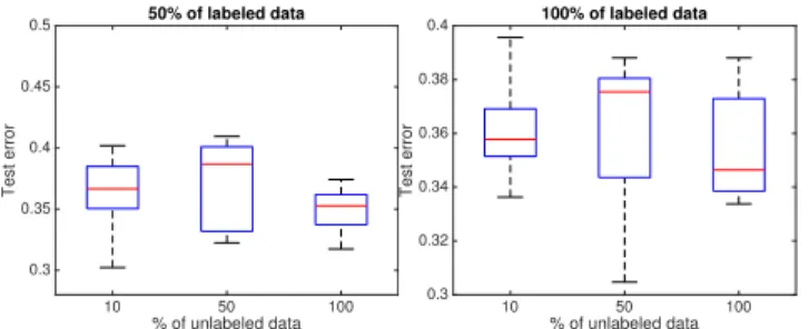
10 50 100 % of unlabeled data 0.3 0.35 0.4 0.45 0.5 Test error 50% of labeled data 10 50 100 % of unlabeled data 0.3 0.32 0.34 0.36 0.38 0.4 Test error 100% of labeled data

Fig. 1. Experiments on the cause-effect pairs. The accuracy of the semi-supervised criterion based on the log-likelihoods with 50% of training data (on the left), and with 100% of training data (on the right).

The pairs 52 – 55, 70 – 71, and 81 – 83 are excluded from the analysis, since they are multivariate problems. Note that each pair is weighted, and the accuracy is a weighted average.

It was reported that Origo [18] achieves 58% accuracy, and the Additive Noise models (ANM) [14] reach 72 ± 6%. We tested the ANM with the Gaussian Process regression which is the state-of-the-art method. The code is publicly available at http://www.math.ku.dk/∼_{peters/code.html.}

The goodness of fit is evaluated by the HSIC independence test of the residuals and the input, and the causal inference is based on the obtained p-values for both directions. The estimated p-values for both directions can be quite similar, and it was, for instance, the case in our experiments. In this situation, although the algorithm infers a causal direction, a natural question arises whether the algorithm has to abstain from taking decisions if the confidence level is low.

To compare to the state-of-the-art, we estimate the func-tional relationships between the cause-effect pairs by the proposed semi-supervised methods. Both settings are devel-oped for discrete data, and we discretize the continuous data using the equal frequency method, the equal width method, and the global equal width method (we use the “infotheo” R package). We also try to find an optimal number of categories for each variable by cross validation; and we test the different number of bins = 3, 5, 7, 10, 15,20, 25, and 30. We decide to fix the number of bins equal to 5.

Figure 1 illustrates the accuracy of the semi-supervised method based on the log-likelihoods, where we applied eq. 10 and eq. 12, as a function of the size of labeled and unlabeled data. We observe that the proposed method achieves the state-of-the-art performance. On the left, we see that increasing the size of unlabeled data, we slightly increase the accuracy and also decrease the variance of the error rate. On the right we observe, that some attention is needed while introducing unlabeled data, since in case where we use 100% of labeled and 100% of unlabeled data, it seems that we overfit.

5.2 Network Reconstruction

We run experiments on two benchmark networks, both downloadable from the Bayesian Network Repository3_:

1) Asia data set [28], also known as the lung cancer benchmark data. The number of nodes is 8, the number of true arcs is 8.

Method Asia Sachs 25 100 1000 25 100 1000 Semi-Sup 0.1560 0.1755 0.3005 0.3510 0.7360 1.1350 DC 0.1595 0.1830 0.3160 0.3645 0.7545 1.1480 RESIT 0.1345 0.3345 28.2935 0.5820 57.1550 163.3755 PC 0.0080 0.0100 0.0130 0.0165 0.0530 0.0645 CPC 0.0100 0.0120 0.0215 0.0260 0.1860 0.2455 LiNGAM 1.7600 1.7020 1.7235 0.0875 0.2245 0.3590 GDS 6.0085 590.9255 590.9255 200.7760 8515.4505 8515.4505 TABLE 1

Runtimes for the tested algorithms: RESIT, LiNGAM, CPC, PC, GDS, DC, and the Semi-Supervised approach on Asia and Sachs with 25, 100, and 1000 generated observations.

● ● ● ● ● ● ● ● ● ● ● 25 RESIT 25 LINGAM 25 CPC 25 PC 25 GDS 25 DistCor

25 SemiSup 100 RESIT _{100 LINGAM} 100 CPC 100 PC 100 GDS

100 DistCor

100 SemiSup 1000 RESIT _{1000 LINGAM} 1000 CPC 1000 PC 1000 GDS 1000 DistCor 1000 SemiSup 0.0 0.2 0.4 0.6 0.8 1.0 Asia FScore ● ● ● ● ● ● 25 RESIT 25 LINGAM 25 CPC 25 PC 25 GDS 25 DistCor

25 SemiSup 100 RESIT _{100 LINGAM} 100 CPC 100 PC 100 GDS

100 DistCor

100 SemiSup 1000 RESIT _{1000 LINGAM} 1000 CPC 1000 PC 1000 GDS 1000 DistCor 1000 SemiSup 0.0 0.2 0.4 0.6 0.8 1.0 Sachs FScore

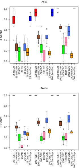
Fig. 2. F-score for the Asia and Sachs data. The number of samples tested is 25, 100, and 1000.

2) Sachs [29] is a causal protein-signalling network with 11 nodes and 17 arcs.

The data sets are network reconstruction challenges with discrete entries. In our experiments, we are interested to discover causality, not the graph structure. We suppose that the skeleton of networks is known, and we compare the causal inference algorithms only.

Aracne (Algorithm for the Reconstruction of Accurate

Cellular Networks) introduced by [30] is a state-of-the-art network information-theoretic reconstruction method. The approach defines an edge in a graph as an irreducible sta-tistical dependency. It is reported that the Aracne achieves very low error rates, however, the reconstructed graph is undirected, therefore the Aracne is unable to infer edge directions. The Aracne, however, can be used to build the graph structure in real applications.

We test RESIT (regression with subsequent indepen-dence test) which is a state-of-the-art ANM method [14]. The RESIT is based on independence tests and simple algorithms that use the independence scores. The algorithm is an itera-tive procedure where at each iteration, a sink node is iden-tified and disregarded. We also test Linear non-Gaussian Acyclic Model (LiNGAM) approach [31], the PC algorithm named after its inventors Peter Spirtes and Clark Glymour [5], its conservative version CPC [32], and the Greedy DAG search algorithm GDS [33]. The implementation of the state-of-the-art methods mentioned above is publicly available from the web page of Jonas Peters4_.

Figure 2 illustrates the performance in terms of F-score on the Asia (above) and Sachs (below) benchmarks. We tested the described above RESIT, LiNGAM, CPC, PC, GDS, Distance Correlation, and the proposed methods. For each benchmark (Asia and Sachs), and for each causal inference method, we tested three scenarios with different number of observations. So, each boxplot shows the results for three settings with various number of data points sampled from the networks (25, 100, and 1000 respectively), and for all causal inference approaches. We run 10 simulations for each setting. The estimated orientations are evaluated for different number of samples. The results are discussed in terms of true positive (TP), false positive (FP) and false negative (FN) edges (i.e. correct, spurious or missing edges respectively). In particular, evaluations are based on Preci-sion = TP/(FP+TP), Recall = TP/(TP+FN), and F-score = 2*Precision*Recall/(Precision+Recall). We observe that the RESIT and the proposed semi-supervised method based on the log-likelihoods achieve the best performance. The Distance Correlation (DC) is less efficient.

5.3 Runtime Results for Network Reconstruction

We have shown that the proposed algorithm achieves the state-of-the-art performance, and sometimes outperforms it in terms of empirical accuracy. Another question is its computational efficiency. Table 1 shows the internal time at

0 800 0.2 0.4 10 600 Test error 0.6 0.8 Bacteria 400 1 % of unlabeled data 200 0 100

Fig. 3. Metformin and bacteria: test error of the semi-supervised (log-likelihood) causal criterion as a function of the amount of unlabeled data.

execution in seconds for different number of tested samples and for different causal methods. The PC and CPC seem to be the fastest to learn but not very accurate. The RESIT shows low error rates but its runtimes increase drasti-cally with the number of observations. The semi-supervised method based on the log-likelihoods and the original dis-tance correlation approach need similar time to learn but our method achieves a better F-score. Note that although the proposed algorithm is already quite efficient, the current implementation of our method is not optimized yet, and it is possible to speed it up. One research avenue is to parallelize the computations what today is actively being studied in the context of deep learning [34], and another future direction is to adopt a quantized deep learning approach that are known to create compact models and to accelerate the runtime [35].

5.4 Effects of Metformin on Human Gut Composition

Recently, a number of associations between chronic human diseases and alterations in gut microbiome composition have been shown [36]. An important question is whether treatment causes changes in human gut flora, and whether it affects metabolism. [36] have reported that the human gut microbiome of type 2 diabetes is confounded by metformin treatment, and therefore, the drug metformin impacts the composition and richness of the human gut microbiome. Similar results were reported by [37].

The data set of [36] which we explore in our experi-ments is a multi-country metagenomic dataset, containing information about patients from three countries: Danemark, China, and Sweden. The data contains information of 106 patients with type 2 diabetes who take the metformin, and 93 patients with the diabetes who does not take the drug. The features are 785 gut metagenomes or gut bacteria.

We run the novel algorithm to test whether it confirms the statements of [36] and [37] that the metformin alters, in other words, impacts, that gut flora. In the numerical experiments, we suppose that the metformin causes changes in bacteria. If an algorithm predicts the inverse, we consider that it makes an error. The observation matrix contains abundance of bacteria. The abundance matrix is a sparse matrix where 1 means that a metagenome is present in a patient, and 0 means that it is absent.

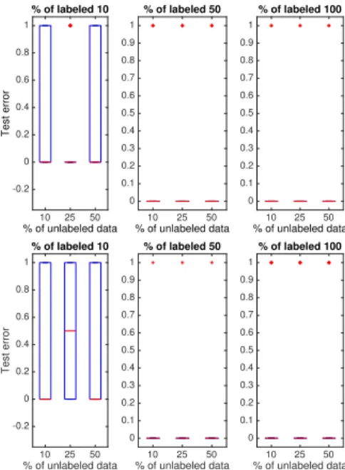
10 25 50 % of unlabeled data -0.2 0 0.2 0.4 0.6 0.8 1 Test error % of labeled 10 10 25 50 % of unlabeled data 0 0.1 0.2 0.3 0.4 0.5 0.6 0.7 0.8 0.9 1 % of labeled 50 10 25 50 % of unlabeled data 0 0.1 0.2 0.3 0.4 0.5 0.6 0.7 0.8 0.9 1 % of labeled 100 10 25 50 % of unlabeled data -0.2 0 0.2 0.4 0.6 0.8 1 Test error % of labeled 10 10 25 50 % of unlabeled data 0 0.1 0.2 0.3 0.4 0.5 0.6 0.7 0.8 0.9 1 % of labeled 50 10 25 50 % of unlabeled data 0 0.1 0.2 0.3 0.4 0.5 0.6 0.7 0.8 0.9 1 % of labeled 100

Fig. 4. Metformin and Akkermansia muciniphila: causality prediction error rate as a function of labeled and unlabeled data. Above: the criterion based on the log-likelihoods; below: the setting based on the distance correlation.

Figure 3 shows that the semi-supervised causal method in generally confirms that the microbiota is affected by the metformin treatment. For the majority of the bacteria considered in the experiments, this relation is obvious with the error rate equal to 0. For a few bacteria the accuracy is not so high. However, [36] and [37] focus on a very limited number of bacteria species, and the statement that the metformin impacts the metagenome is not necessarily true for all bacteria of the human gut flora. Figure 4 illustrates the error rate for one particular bacterium called Akkermansia muciniphila which is associated with the metabolic health. We clearly see that the hypothesis that the metformin alters the abundance of Akkermansia muciniphila is verified by both proposed semi-supervised settings.

6

C

We challenged the problem of causal relations discovery from purely observational non-temporal data. In this con-tribution, we introduced a novel causal inference approach based on a semi-supervised probabilistic framework. The advantage of our approach is its high efficiency, and high computational speed. Note that its implementation is simple and straightforward.

We have compared the proposed semi-supervised causal inference algorithm to the state-of-the-art methods, and we illustrate by the experiments on standard data sets and benchmark networks (discrete or discretized data) that the approach achieves the best performance in terms of F-score and accuracy. We have shown that the proposed method is efficient to detect whether a drug causes alterations in the human gut.

It is quite challenging to claim that this or that bacterium is influenced by metformin or another drug. Even if we observe a strong causal relation, we need a validation from

scientists doing pre-clinical research. However, it is among our plans in the nearest future to consider more bacteria or even a cumulative effect of a drug on several bacteria which are in the same environmental niche.

From the results of our experiments, we can conclude that measuring distance between a supervised and an un-supervised models can indeed provide information on the edge orientation.

Currently we are investigating another scheme of causal inference which is based on generative hierarchical prob-abilistic models. We are also interested to extend the pro-posed method for confounding variables.

R

[1] R. Shaw et al., “The kinase lkb1 mediates glucose homeostasis in

liver and therapeutic effects of metformin,” Science, vol. 310, pp. 1642–1646, 2005.

[2] A. Madiraju et al., “Metformin suppresses gluconeogenesis by

in-hibiting mitochondrial glycerophosphate dehydrogenase,” Nature, vol. 510, pp. 542–546, 2014.

[3] L. McCreight, C. J. Bailey, and E. Pearson, “Metformin and the

gastrointestinal tract,” Diabetologia, vol. 59, pp. 426–435, 2016.

[4] J. Pearl, Causality: Models, Reasoning and Inference. Cambridge

University Press, 2nd edition, 2009.

[5] P. Spirtes, C. Glymour, and R. Scheines, Causation, Prediction, and Search. MIT Press, 2000.

[6] D. Janzing and B. Sch ¨olkopf, “Causal inference using the algorith-mic Markov condition,” IEEE Transactions on Information Theory, vol. 56, pp. 5168–5194, 2010.

[7] D. Janzing, J. Mooij, K. Zhang, J. Lemeire, J. Zscheischler, P. Da-niusis, B. Streudel, and B. Sch ¨olkopf, “Information-geometric ap-proach to inferring causal directions,” Artificial Intelligence, 2012. [8] E. Sgouritsa, D. Janzing, P. Hennig, and B. Sch ¨olkopf, “Inference

of cause and effect with unsupervised inverse regression,” in AISTATS, 2015.

[9] S. Affeldt, L. Verny, and H. Isambert, “3off2: A network

recon-struction algorithm based on 2-point and 3-point information statistics,” BMC Bioinformatics, vol. 17, no. S-2, p. 12, 2016.

[10] I. Goodfellow, Y. Bengio, and A. Courville, Deep Learning. MIT

Press, 2016.

[11] R. Salakhutdinov and G. Hinton, “Deep Boltzmann machines,” in AISTATS, 2009.

[12] J. M. Mooij, J. Peters, D. Janzing, J. Zscheischler, and B. Sch ¨olkopf, “Distinguishing cause from effect using observational data: meth-ods and benchmarks,” JMLR, vol. 17, 2016.

[13] P. Hoyer, D. Janzing, J. Mooij, J. Peters, and B. Sch ¨olkopf, “Nonlin-ear causal discovery with additive noise models.” in NIPS, 2009. [14] J. Peters, J. Mooij, D. Janzing, and B. Sch ¨olkopf, “Causal discovery

with continuous additive noise models,” JMLR, vol. 1, no. 15, pp. 2009–2053, 2014.

[15] K. Zhang and A. Hyv¨arinen, “On the identifiability of the post-nonlinear causal models,” in UAI, 2009.

[16] P. B ¨uhlmann, J. Peters, and J. Ernest, “Cam: Causal additive models, high-dimensional order search and penalized regression.” Annals of statistics, vol. 42, pp. 2526–2556, 2014.

[17] J. Zscheischler, D. Janzing, and K. Zhang, “Testing whether linear equations are causal: a free probability theory approach,” in UAI, 2009.

[18] K. Budhathoki and J. Vreeken, “Causal inference by compression,” in ICDM, 2016.

[19] C. Louizos, U. Shalit, J. Mooij, D. Sontag, R. Zemel, and M. Welling, “Causal effect inference with deep latent-variables models,” in NIPS, 2017.

[20] E. Sgouritsa, D. Janzing, J. Peters, and B. Sch ¨olkopf, “Identifying finite mixtures of nonparametric product distributions and causal inference of confounders,” in Proceedings of the 29th Annual Con-ference on Uncertainty in Artificial Intelligence (UAI). AUAI Press, 2013, pp. 556–565.

[21] F. Liu and L. Chan, “Causal inference on discrete data via estimat-ing distance correlations,” Neural Computation, vol. 28, 2016. [22] K. Pearson, “Notes on the history of correlation,” Biometrika,

vol. 13, pp. 25–45, 1920.

[23] N. Sokolovska, O. Capp´e, and F. Yvon, “The asymptotics of semi-supervised learning in discriminative probabilistic models,” in ICML, 2008.

[24] B. Sch ¨olkopf, J. D., J. Peters, E. Sgouritsa, and K. Zhang, “On causal and anticausal learning,” in ICML, 2012.

[25] G. Hinton, S. Osindero, and Y. W. Teh, “A fast learning algorithm for deep belief nets,” Neural Computation, vol. 18, no. 7, pp. 1527– 1554, 2006.

[26] R. Salakhutdinov and H. Larochelle, “Efficient learning of deep Boltzmann machines,” in AISTATS, 2010.

[27] R. Salakhutdinov and I. Murray, “On the qualitative analysis of deep belief networks,” in ICML, 2008.

[28] S. Lauritzen and D. Spiegelhalter, “Local computation with prob-abilities on graphical structures and their application to expert systems,” Journal of the Royal Statistical Society: Series B (Statistical Methodology), vol. 2, no. 50, pp. 157–224, 1988.

[29] K. Sachs, O. Perez, D. Pe’er, D. Lauffenburger, and G. Nolan, “Causal protein-signaling networks derived from multiparameter single-cell data,” Science, vol. 308, pp. 523–529, 2005.

[30] A. Margolin, I. Nemenman, K. Basso, C. Wiggins, G. Stolovitzky, R. Favera, and F. Califano, “Aracne: an algorithm for the recon-struction of gene regulatory networks in a mammalian cellular context,” BMC Bioinformatics, 2006.

[31] S. Shimizu, O. Hoyer, A. Hyv¨arinen, and J. Kerminen, “A linear non-gaussian acyclic model for causal discovery,” JMLR, vol. 7, pp. 2003–2030, 2006.

[32] J. Ramsey, J. Zhang, and P. Spirtes, “Adjacency-faithfulness and conservative causal inference,” in UAI, 2006.

[33] A. Hauser and P. B ¨uhlmann, “Characterization and greedy learn-ing of interventional markov equivalence classes of directed acyclic graphs,” JMLR, vol. 13, pp. 2409–2464, 2012.

[34] T. Ben-Nun and T. Hoefler, “Demystifying parallel and dis-tributed deep learning: an in-depth concurrency analysis,” in https://arxiv.org/pdf/1802.09941, 2018.

[35] Y. Xu, Y. Wang, A. Zhou, W. Lin, and H. Xiong, “Deep neural net-work compression with single and multiple level quantization,” in AAAI, 2018.

[36] K. Forslund, F. Hildebrand, T. Nielsen, G. Falony, E. L. Chatelier, S. Sunagawa, E. Prifti, S. Viera-Silva, V. Gudmundsdottir, H. K. Pedersen, M. Arumugam, K. Kristiansen, A. Y. Voigt, H. Vester-gaard, R. Hercog, P. I. Costea, J. R. Kultima, J. Li, T. Jorgensen, F. Levenez, J. Dore, M. consortium, H. B. Nielsen, S. Brunak, J. Raes, T. Hansen, J. Wang, S. D. E. und P. Bork, and O. Pedersen, “Disentangling the effects of type 2 diabetes and metformin on the human gut microbiota,” Nature, vol. 7581, no. 528, 2015.

[37] H. Wu, E. Esteve, V. Tremaroli, M. Khan, R. Caesar, L. Manneras-Holm, M. Stahlman, L. Olsson, M. Serino, M. Planas-Felix, G. Xifra, J. Mercader, D. Torrents, R. Burcelin, W. Ricart, R. Perkins, J. Fernandez-Real, and F. Backhed, “Metformin alters the gut mi-crobiome of individuals with treatment-naive type 2 diabetes, con-tributing to the therapeutic effects of the drug,” Nature Medicine, vol. 7, no. 23, 2017.