Studying dynamics without explicit dynamics: a structure-based study of the export mechanism by AcrB
Texte intégral
Figure

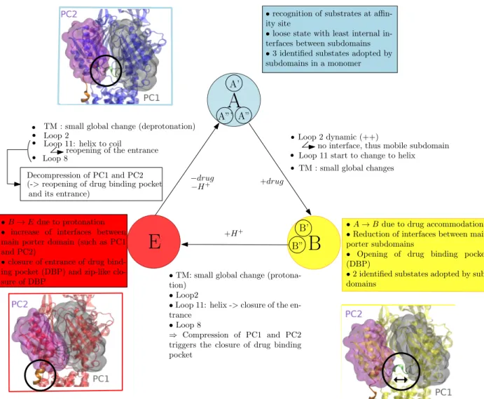

![Figure 8: Mechanism for the trimer (Adapted from [5]) Schematic representation of the AcrB alternating site functional rotation transport mechanism extended by postulated intermediate steps.](https://thumb-eu.123doks.com/thumbv2/123doknet/12959358.376641/40.918.285.637.329.662/mechanism-schematic-representation-alternating-functional-transport-postulated-intermediate.webp)
Documents relatifs
In terms of solution accu- racy, that is to say the mean quadratic deviation between modelled and experimental points, the solutions obtained in this study are about 10 times as
9 shows how the incorporation of new hardware to the on-orbit facility can enable further testing that increases the direct traceability of the testbed to future
form and a connection preserving it make such a quantization triple which is easily associated with a twisted quantization triple and hence gives a map from
This PhD thesis has proposed contributions to the development of new alternative renewable energy generation using wind. The original idea was very simple: replace the heavy and
On appelle fonction homographique toute fonction h non affine qui peut s'écrire comme quotient de deux fonctions affines... On désigne par x la distance DM exprimée
ClayFF and ClayFF MOD, the water oxygen atoms had only a slightly higher probability of presence above the center of the hexagonal sur- face cavities (Fig. 3a and Fig. 3b; note that
2014 A general analytic and very rapid method for the calculation of the mean square vibration amplitude of crystal atoms is given.. This method has been tested on a
In the crystal phases of D-BPBAC and D-IBPBAC no quasi-elastic broadening was observed indicating that there are no diffusive motions of the cores of the molecules
