Using meta-models for tsunami hazard analysis: an example of application for the French Atlantic Coast.

HAL Id: hal-03103034

https://hal.archives-ouvertes.fr/hal-03103034

Submitted on 7 Jan 2021

HAL is a multi-disciplinary open access

archive for the deposit and dissemination of

sci-entific research documents, whether they are

pub-lished or not. The documents may come from

teaching and research institutions in France or

abroad, or from public or private research centers.

L’archive ouverte pluridisciplinaire HAL, est

destinée au dépôt et à la diffusion de documents

scientifiques de niveau recherche, publiés ou non,

émanant des établissements d’enseignement et de

recherche français ou étrangers, des laboratoires

publics ou privés.

example of application for the French Atlantic Coast.

Vito Bacchi, Herve Jomard, Oona Scotti, Ekaterina Antoshchenkova, Lise

Bardet, Claire Marie Duluc, Hélène Hebert

To cite this version:

Vito Bacchi, Herve Jomard, Oona Scotti, Ekaterina Antoshchenkova, Lise Bardet, et al.. Using

meta-models for tsunami hazard analysis: an example of application for the French Atlantic Coast..

Frontiers in Environmental Science, Frontiers, 2020, 8, �10.3389/feart.2020.00041�. �hal-03103034�

in Earth Science

r®i

Using Meta-Models for Tsunami

Hazard Analysis: An Example of

Application for the French Atlantic

Coast

Vito Bacchi1*, Hervé Jomard1, Oona Scotti1, Ekaterina Antoshchenkova1, Lise Bardet1, Claire-Marie Duluc1 and Hélène Hebert2

1 Institute for Radiological Protection and Nuclear Safety, Fontenay-aux-Roses, France,2 CEA, DAM, DIF, Arpajon, France

OPEN ACCESS

Edited by:

Philippe Renard, Université de Neuchâtel, Switzerland

Reviewed by:

Jacopo Selva, Istituto Nazionale di Geofisica e Vulcanologia (INGV), Italy Tipaluck Krityakierne, Mahidol University, Thailand

*Correspondence:

Vito Bacchi vito.bacchi@gmail.com

Specialty section:

This article was submitted to Solid Earth Geophysics, a section of the journal Frontiers in Earth Science

Received: 08 May 2019 Accepted: 04 February 2020 Published: 03 March 2020

Citation:

Bacchi V Jomard H, Scotti O, Antoshchenkova E, Bardet L, Duluc C-M and Hebert H (2020) Using Meta-Models for Tsunami Hazard Analysis: An Example of Application for the French Atlantic Coast. Front. Earth Sci. 8:41. doi: 10.3389/feart.2020.00041

This paper illustrates how an emulator (or meta-model) of a tsunami code can be a useful tool to evaluate or qualify tsunami hazard levels associated with both specific and unknown tsunamigenic seismic sources. The meta-models are statistical tools permitting to drastically reduce the computational time necessary for tsunami simulations. As a consequence they can be used to explore the tsunamigenic potential of a seismic zone, by taking into account an extended set of tsunami scenarios. We illustrate these concepts by studying the tsunamis generated by the Azores-Gibraltar Plate Boundary (AGPB) and potentially impacting the French Atlantic Coast. We first analyze the impact of two realistic scenarios corresponding to potential sources of the 1755-Lisbon tsunami (when uncertainty on seismic parameters is considered). We then show how meta-models could permit to qualify the tsunamis generated by this seismic area. All the results are finally discussed in light of tsunami hazard issued by the TSUMAPS-NEAM research project available online (http://ai2lab.org/tsumapsneam/ interactive-hazard-curve-tool/). From this methodological study, it appears that tsunami hazard issued by TSUMAPS-NEAM research project is envelop, even when compared to all the likely and unlikely tsunami scenarios generated in the AGPB area.

Keywords: kriging surrogate, uncertainty quantification, tsunami modeling, hazard analysis, sensitivity analysis

INTRODUCTION

The évaluation of tsunami impact requires accurate simulation results for planning and risk assessment purposes because of the severe consequences which could be associated to this kind of event. Considering that tsunami phenomena involve a large span of parameters at different spatial and temporal scales (Behrens and Dias, 2015), even a single run of a tsunami numerical model can

Abbreviations: p, shear modulus; [N(m(x), s2 (x))], Gaussian process of mean “m(x)” and variance “s2(x)”; [M(x)], kriging

surrogate; {X,Y}, are the coordinates of the design simulations used for kriging parameters evaluation; C(.), covariance kernel; CEA, commissariat à l'énergie atomique et aux énergies alternatives; D [m], average slip along the rupture surface; DTHA, deterministic tsunami hazard assessment; GSA, global sensitivity analysis; L [m], length of the rupture surface; MCS, maximum credible scenario; MCS_h, tsunami hazard level issued by an exploration of a very wide range of tsunamigenic scenarios; Mo, seismic moment; Mw, seismic moment magnitude; MSE, mean squared error; PTHA, probabilistic tsunami hazard assessment; R2, squared correlation coefficient; RMSE, root mean squared error; UQ, uncertainty quantifications; W [m], width of the rupture surface.

be prohibitively long, in the order of minutes to days, according to the study area characteristics and to the resolution of the numerical model. Hence, a common practice when the computational code is time-consuming is the use of meta-models (also denoted surrogate-models or emulators). A meta-model is a mathematical model of approximation of the numerical model, built on a learningbasis (Razavi et al., 2012a). Meta-models have been applied, for example, in hydraulic fields to model physical variables such as flows (Wolfs et al., 2015; Machac et al., 2016), flood damages (Yazdi and Salehi Neyshabouri, 2014), or in the field of the design for civil flood defenses (Richet and Bacchi, 2019). A comprehensive review of the use of meta-models in environmental research was proposed by Razavi et al. (2012a) for the interested reader.

Meta-models have also already been used in the field of tsunamis. For instance, Sraj et al. (2014) investigate the uncertainties in the resulting wave elevation predictions due to the uncertainty in the Manning’s friction coefficient, using polynomial chaos expansion to build a surrogate model that is a computationally cheap approximation of the computer model. Sarri et al. (2012) used in a similar way a statistical emulator of the analytical landslide-generated tsunami model developed by Sammarco and Renzi (2008). More recently, Rohmer et al. (2018) studied the uncertainty related to the source parameters through a Bayesian procedure to infer (i.e., learn) the probability distribution ofthe source parameters ofthe earthquake. However, to our knowledge, meta-modeling has never been used for tsunami hazard analysis.

In this paper, we propose to apply meta-modeling techniques in the framework of deterministic tsunami hazard assessment (DTHA) and evaluate how it can be useful in seismic areas with no (or poor) seismotectonic knowledge. In such cases, when seismotectonic parameters are uncertain, it may be of interest to provide a first order idea of the tsunami hazard potential through DTHA, the implementation of DTHA being simpler than the probabilistic method (PTHA). The scenario-based (or DTHA) approach classically relies on the study of “maximum credible scenarios” (MCS). In particular, DTHA tries to explore the potential of the largest scenarios, by selecting some of the extreme ones (i.e., a recorded/reconstructed historical event) and simulating them for the target area through numerical modeling (JSCE, 2002; Lynett et al., 2004), without addressing the likelihood of occurrence of such a big event (Omira et al., 2016). With this approach, MCS is assessed through an expert opinion. The outputs of the deterministic analysis are, in general, tsunami travel time, wave height, flow depth, run-up, and current velocity maps corresponding to the chosen scenario (Omira et al., 2016).

As mentioned above, DTHA relies on a refined knowledge of the seismic sources generating the tsunamis. As a consequence, it could be hampered by the use of specific values of input parameters which may be subjective depending on the person or group carrying out the analysis (Roshan et al., 2016). A good example is the 1755 Lisbon tsunami, generated by an earthquake in the Azores Gibraltar Plate Boundary (AGPB). The Great 1755 Lisbon earthquake generated the most historically destructive tsunami near the Portugal coasts (Santos and Koshimura, 2015). Source location and contemporary effects of such tsunami are not

precisely identified and several earthquake scenarios have already been published in the literature in the last decades (Johnston, 1996; Baptista et al., 1998, 2003; Zitellini et al., 1999; Gracia et al., 2003; Terrinha et al., 2003; Gutscher et al., 2006; Grandin et al., 2007; Horsburgh et al., 2008; Barkan et al., 2009; Cunha et al., 2010). All of these studies show how variable the parameters of the seismic source can be and the importance to take into account their uncertainty.

In DTHA, the classical approach to deal with uncertainties consists in performing a limited number of deterministic simulations with conservative values of the seismic sources (e.g., JSCE, 2002; Lynett et al., 2004; Allgeyer et al., 2013). However, the great M 9.0 Tohoku-Oki subduction earthquake of 2011, the largest ever recorded in Japan (Saito et al., 2011), has clearly shown the limitations of the classical approach focused on the identification of known maximum tsunamigenic sources (MCS approach). Recently, Roshan et al. (2016) improved the DTHA procedure detailed in Yanagisawa et al. (2007) in order to better evaluate the effects of the seismic source uncertainties through Monte-Carlo simulations of a limited number of seismic source parameters (the dip angle, the strike and the source location), leading to around 300 tsunami scenarios. The authors presented an improvement of the classical MCS approach by introducing uncertainties on seismic source parameters.

In this context, the objective of this work is to propose a new methodology to evaluate or qualify tsunami hazard levels associated to both specific and unknown tsunamigenic seismic sources by integrating the uncertainty related to the seismic parameters in the DTHA procedure. The main idea is to develop a meta-model, or emulator, of the tsunami numerical model, that makes it possible to perform a large number of tsunami scenarios with reduced computational time and, consequently, to intensively explore a tsunamigenic area for which geological and geophysical datasets may be limited. The constructed meta- models, when exploited with the statistical criteria classically employed in uncertainty quantification (UQ) studies (Saltelli et al., 2000, 2008; Saltelli, 2002; Iooss and Lemaître, 2015), can permit to go beyond the classical approach for DTHA and perform a better quantification of uncertainties of a large set of seismic source parameters.

In the next sections we will first present the methodology used in this study (see section “Methodology”), and then develop and validate the meta-models for AGPB related tsunamis impacting the French Atlantic Coast (see section “Application of the methodology to the French Coast”). In section “Potential application of meta-models for tsunami hazard analysis,” we (1) evaluate the impact of two realistic scenarios corresponding to potential sources of the 1755-Lisbon tsunami (when uncertainty on seismic parameters is considered), and (2) present the analysis of the tsunamigenic potential of the AGPB zone, considered for the purpose of the exercise as a poorly known tsunamigenic area. Finally, we show how the numerical results obtained with this method can be discussed in light of tsunami hazard issued by the TSUMAPS-NEAM research project available on line1.

METHODOLOGY

The proposed approach relies on three main steps, as reported in Figure 1. STEP 1 consists in the construction of a numerical model able to reproduce the tsunami heights generated by a given seismic area and impacting a target area. In STEP 2, the numerical model simulates a regular set of physical tsunamigenic scenarios (so called design data-base) that are used for the construction and the validation of an emulator (the meta-model) able to reproduce the original model results in the target zone. In STEP 3, the validated meta-models may be used for DTHA assessment and/or qualification of other THA results. The UQ performed using meta-models instead of the original model permits to assess the uncertainty related to a given tsunami scenario (see section “In the case of expert opinion: uncertainty quantification in DTHA”) and to explore intensively the tsunamigenic area with nearly zero computational time (see section “Without expert opinion: exploration of a large tsunamigenic area”).

Step 1: Tsunami Simulations

The first step consists in the construction of a tsunami numerical model of the area to explore. In this study, the tsunami numerical simulations were performed by using the tsunami code reported in Allgeyer et al. (2013) (or CEA-code), which exploits two models, one for tsunami initialization and the other one for tsunami propagation. The initial seabed deformation caused by an earthquake is generated with the Okada model (Okada, 1985) and is transmitted instantaneously to the surface of the water.

FIGURE 1 | Global methodology proposed in this study.

This analytical model uses simplistic planar fault parameters with uniform slip, satisfying the expression of the seismic moment Mo:

M0 = p ■ D ■ L ■ W (1) where ^ denotes the shear modulus, D [m] the average slip along the rupture of length L [m] and width W [m]. Then, the seismic moment magnitude “Mw” is directly computed through equation 2 (Hanks and Kanamori, 1979), as follow:

2

Mw = 3 ■ logw(M0) - 6, 07 (2) The following parameters are also required for tsunami initiation:

longitude, latitude, and depth [km] of the center of the source, strike [degrees], dip [degrees], and rake [degrees]. A conceptual

scheme of the input parameters for the tsunami-code and the numerical domain used in this study are reported in Figure 2. Then, the computation of the tsunami propagation is based on hydrodynamic equations, under the non-linear shallow water approximation (the Boussinesq equations as reported in Allgeyer et al., 2013). Shallow water equations are discretized using a finite-differences method in space and time (FDTD). Pressure and velocity fields are evaluated on uniform separate grids according to Arakawa's C-grid (Arakawa, 1972). Partial derivatives are approximated using upwind finite- differences (Mader, 2004). Time integration is performed using the iterated Crank-Nicholson scheme. No viscosity terms are taken into account in our simulations. The only parameters of this model are the bathymetry (space step and depth resolution) and the time step.

Step 2: Meta-Model Design and

Validation

Meta-Models Design

A variety of metamodels have been applied in the water resources literature (Santana-Quintero et al., 2010; Razavi et al., 2012b). Moreover, some examples of applications have already been published in the context of flood management (e.g., Yazdi and Salehi Neyshabouri, 2014; Lowe et al., 2018) and in the field of tsunamis (e.g., Sarri et al., 2012; Sraj et al., 2014; Rohmer et al., 2018). The classical steps for meta-models construction and validation are reported in various studies (i.e., Saltelli, 2002; Saltelli et al., 2008; Faivre et al., 2013), and are shortly summarized in Table 1.

For the study presented here, we rely on conditional Gaussian processes (also known as kriging (Roustant et al., 2012), derived from Danie Kriges pioneering work in mining (Krige, 1951), later formalized within the geostatistical framework by Matheron (1963). Kriging meta-model has already shown good predictive capacities in many practical applications (see Marrel et al., 2008, for example), it became a standard meta-modeling method in operational research (Santner et al., 2003; Kleijnen, 2005) and it has performed robustly in previous water resource applications (Razavi et al., 2012b; Villa-Vialaneix et al., 2012; Lowe et al., 2018).

A general kriging model “M(x)” (which later provides an estimation of the maximum tsunami height in a given location)

FIGURE 2 | (A) Numerical domain used for the deterministic simulations performed in this study and (B) geometrical input parameters of the tsunami-code employed in the study d [km] is the depth of the seismic source which is assumed to be at the middle of the fault, hL [km] is the half fault length, W [km] is the half fault width, x-y-z are three-dimensional axes.

can be defined for x = (x1,..., ) e D e Rd as the following Gaussian process “N(.)”:

M(x) = N(m(x), s2 (x))

Where, for simple kriging:

- m(x) = C(x)TC(X)—1Y is the conditional mean;

TABLE 1 | Steps for meta-models construction, validation and evaluation of the uncertainty.

Step for Description meta-models design

Initial design database

Construction

Accuracy/Optimization

Meta-model uncertainty

Monte-Carlo sampling in the distribution of the model input parameters.

Estimation of meta-model parameters according to equations reported in section “Meta-models design” using training set data base

k-fold cross validation (Breiman and Spector, 1992; Kohavi, 1995; Hastie et al., 2009).

RMSE and R2 issued from the Accuracy/Optimization step.

- s2(x) = c(x) — C(x)TC(X)—1 C(x) is the conditional variance;

- C : (u, v) e D2 ^ C(u, v) e R is the covariance Kernel; - c(x) is the vector of covariance between the kriging

predictions and the original model evaluations.

It must be noted that {X,Y} are the coordinates of the design simulations used for kriging parameters evaluation:

- X is a matrix containing for each design simulation (for a total of N simulations) the value of the seismic source model parameters defined in section “Step 1: tsunami simulations” (for a total of 9 inputs parameters):

x1,1 . . . x1,9

X=

xN,9 . . . xN,9

- Y is a vector containing, for each gauge, the maximum water depth associated to a simulation:

hmax, 1

hmax,N

More than a commonplace deterministic interpolation method (like splines of any order) this model is much more informative owing to its predicted expectation and uncertainty. The fitting procedure of this model includes the choice of a covariance model

[here a tensor product of the “Matern52” function (Roustant

et al., 2012)], and then the covariance parameters (e.g., range of covariance for each input variable, variance of the random process, nugget effect), could be estimated using Maximum Likelihood Estimation (standard choice we made) or Leave-One- Out minimization [known to mitigate the arbitrary covariance function choice (see Bachoc, 2013)].

It must be noted that the kriging interpolation technique requires computing and inverting the n x n covariance matrix C(X, X) between the observed values Y(X), which leads to

a O(n2) complexity in space and O(n3) in time (Rullière

et al., 2018). In practice, this computational burden makes Gaussian process regression difficult to use when the number of observation points is in the range [103,104] or greater, as in this study. As a consequence, we used in this article the procedure for estimating the parameters of kriging reported in Rullière et al. (2018), by using an adapted R-tool available on line2. The full details of this methodology are reported in the abovementioned paper. This approach is proven to have better theoretical properties than other aggregation methods that can be found in the literature, and permitted us to drastically reduce the computational time necessary for meta- models construction and validation.

Meta-Models Validation

A general method for meta-models validation is the K-fold cross- validation method (Friedman et al., 2001). The principle of cross- validation is to split the data into K folds of approximately equal size A1A1,.. .,AkAk. For k = 1 to K, a model Y(-k) is fitted from the data Uj=kAk (all the data except the Ak fold) and this model is validated on the fold Ak. Given a criterion of quality L as the Mean Square Error:

1 n

L = MSE = (y - y)2 (3) n

the quantity used for the “evaluation” of the model is computed

as follow: 1

Lk = 7K Z L(yiY(-k)(x«)), (4)

n/K ;i€AK

where yi and yi are, respectively, the meta-model and the model response and n is the number of simulations in the kth sample. When K is equal to the number of simulations of the training set, the cross-validation method corresponds to the leave-one-out technique not performed in this study. The methodology employed is described in the DiceEval R-package reference-manual (Dupuy et al., 2015). In our application case, we considered K = 10.

In this study, the accuracy of the meta-model is evaluated through several statistical metrics permitting to quantify the overall quality of regression models. This includes:

- R-squared (R2), representing the squared correlation between the observed outcome values and the values predicted by the model. The higher the adjusted R2 is, the better the model is;

- Root Mean Squared Error (RMSE), which measures the average prediction error made by the model in predicting the outcome for an observation. It corresponds to the average différence between the observed known outcomes and the values predicted by the model. The lower the RMSE is, the better the model is.

Step 3: Uncertainty Quantification and

Global Sensitivity Analysis

Considering the variety and the complexity of the geophysical mechanisms involved in tsunami generation, tsunami hazard assessment is generally associated with strong uncertainties (aleatory and epistemic). In PTHA, uncertainties are classically integrated in a rigorous way (Sorensen et al., 2012; Horspool et al., 2014; Selva et al., 2016) and quantified using the logic- tree approach (Horspool et al., 2014) and/or random simulations performed using the Monte-Carlo sampling of probability density functions of geological parameters (Sorensen et al., 2012; Horspool et al., 2014). An alternative and interesting approach was recently proposed by Selva et al. (2016), consisting in the use of an event tree approach and ensemble modeling (Marzocchi et al., 2015). Moreover, a new procedure was recently proposed by Molinari et al. (2016) for the quantification of uncertainties related to the construction of a tsunami data-base based on the quantification of elementary effects.

In this work we propose a classical methodology that could also be adapted to analyze tsunamigenic regions with poor (or no) information on crustal characteristics and based on the classical uncertainty study steps (Saltelli et al., 2004, 2008; Faivre et al., 2013; Iooss and Lemaître, 2015). This methodology, which was already tested in other hydraulic context in recent years (Nguyen et al., 2015; Abily et al., 2016), relies on Monte Carlo simulations for UQ steps and on GSA (Global Sensitivity Analysis) approaches for the analysis of the AGPB tsunamigenic potential, by computing Sobol indices (Sobol, 1993, 2001). These methods rely on sampling based strategies for uncertainty propagation, willing to fully map the space of possible model predictions from the various model uncertain input parameters and then, allowing to rank the significance of the input parameter uncertainty contribution to the model output variability (Baroni and Tarantola, 2014). The objectives with this approach are mostly to identify the parameter or set of parameters which significantly impact model outputs (Iooss et al., 2008; Volkova et al., 2008). GSA approaches are robust, have a wide range of applicability, and provide accurate sensitivity information for most models (Adetula and Bokov, 2012). Moreover, even if they are theoretically defined for linear mathematical systems, it was demonstrated that they are well suited to be applied with models having non-linear behavior and when interactions among parameters occur (Saint-Geours, 2012), as in the present study. For these reasons, these indices were already adopted for the analysis of bi-dimensional hydrodynamic simulations in urban areas (Abily et al., 2016) or of complex coastal models including interactions between waves, current and vegetation (Kalra et al., 2018) and they seem well suited for the present work.

For the computation of Sobol’ indices, a large variety of methodologies are available, as the so-called “extended- FAST” method (Saltelli et al., 1999), already used in previous studies by IRSN (Nguyen et al., 2015). In this study, we used the methodology proposed by Jansen et al. (1994) already implemented in the open source sensitivity-package R (Pujol et al., 2017). This method estimates first order and total Sobol’ indices for all the factors “v” at higher total cost of “v x (p + 2)” simulations (Faivre et al., 2013).

APPLICATION OF THE METHODOLOGY

TO THE FRENCH COAST

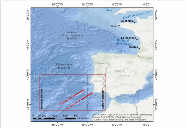
The French Atlantic coast is subjected to two main seismogenic sources that could generate tsunamis, one in the lesser Indies, and a second one from the AGPB. In this application we only consider the AGPB and we only compute water heights offshore for four locations (Figure 3), ignoring the necessary refinements for propagation to the coast. Because in this study case the sources are far from the considered gauges, we propose a very simplified approach to characterize the source region. In the following we first present how the meta-model was constructed and validated through a series of statistical tests in comparison with published data from Allgeyer et al. (2013).

FIGURE 3 | Bathymetry covering the computational domain. Red cross hatching area shows location of tsunamigenic sources used for meta-models construction. The points represent the gauge locations selected for tsunami database construction along the French Atlantic Coast. Gorringe fault and Horseshoe fault are special structures at the boundary between the Eastern domain (on the right) and the Western domain (on the left).

Numerical Tool and Design Data-Base

All the simulations were performed on the same bathymétrie grid with a space resolution of 2’ (~3.6 km). The numerical model was not direetly validated by the eomparison with similar simulations from literature. In faet, eonsidering the rough bathymetrieal grid resolution, the developed numerieal model is not adapted to the estimation of the tsunamis run-up and the inundation areas and it ean’t be used for a real assessment of the tsunami hazard along the Freneh Atlantie Coast. However, this work being methodologieal, we eonsider that the numerieal results are eonsistent with the objeetives of the study. Moreover, the tsunami-eode was largely validated through extensive benehmarks in the framework of the TANDEM researeh projeet (Violeau et al., 2016) by ensuring its ability to reproduee tsunamis generation and propagation. As a eonsequenee, the order of magnitude of the tsunami heights eomputed in this study should be realistie and adapted to the test of the methodology.

In order to perform the numerieal simulations needed for the meta-model eonstruetion and validation (see seetion “Step 2: meta-model design and validation”), the CEA-eode

was eoupled with the IRSN Promethee beneh. Promethee is an environment for parametrie eomputation that allows earrying out UQ studies, when eoupled (or warped) to a eode. This software is freely distributed by IRSN3 and allows the parameterization with any numerieal eode and is optimized for intensive eomputing. Promethee was first linked to the numerieal eode by means of a set of software links (similar to bash seripts). In this way, numerieal simulations were direetly lunehed by the IRSN environment. Then, the statistieal analysis, sueh as the Monte-Carlo simulations used for the meta-model eonstruetion (see seetion “Meta-models design”) and UQ (see seetion “Analysis of the Impaet of Tsunamis on a Target Area through UQ”) or the Sobol indiees eomputation (see seetion “Global Analysis of Seismie Souree Influenee on the Target Area”) were also driven by Promethee, whieh integrates R statistieal eomputing environment by permitting this kind of analysis (R Core Team, 2016).

In this methodologieal work, we eonsidered a widened AGPB tsunamigenie area and we ehose to explore as largely as possible 3http://promethee.irsn.org/doku.php

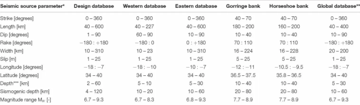
TABLE 2 | Summary of the variation range of the seismic source input parameters for the design, the western, the eastern database and for the tsunami scenarios associated to the Gorringe bank and the Horseshoe bank (hypothesis from Duarte et al., 2013; Grevemeyer et al., 2017).

Seismic source parameter* Design database Western database Eastern database Gorringe bank Horseshoe bank Global database’

Strike [degrees] 0-360 0 - 360 0 - 360 40 - 70 40 - 70 0 - 360 Length [km] 40 - 600 40 - 227 40 - 600 180-200 160-200 40 - 400 Dip [degrees] 1 -90 60 - 90 10 - 90 10-40 10-40 10-90 Rake [degrees] _{-180 : +180 -180 : 0 0 : +180 70 : 110 70 : 110 -180 : +180} Width [km] _{10-310 10-23 10-310 16-224 16-228 20 - 200} Slip [m] 1 -25 1 -25 1 -25 5 - 25 5 - 25 1 -25 Longitude [degrees] -18 : -7 -18 : -10 -10 : -7 -12 : -11 -10.5 : -9.5 -18 : -7 Latitude [degrees] 34 - 40 34 - 40 34 - 40 36.5-37.5 35.8-36.5 34 - 40 Depth*** [km] 2 - 60 5-10 5 - 30 10-40 10-40 5 - 30 Sismogenic depth [km] 4-120 10-20 10 - 60 20 - 80 20 - 80 10-60 Magnitude range Mw [-] 6.7-9.3 6.7-8.3 6.8-9.3 7.7-8.9 7.7-8.9 6.7-9.3

*Seismic source parameters are assumed uniformly distributed and are randomly sampled for the construction of the Global database. **The global database is composed of the scenarios simulated with the meta-models (more than 50,000 tsunamis scenarios) for the construction of the western and the eastern database. ***Note that depth

is considered to be the depth of the seismic source which is assumed to be in the middle of the fault (see Figure 2).

the potential tsunami height along the French Atlantic Coast generated by earthquakes from 34° to 40°N and from 18 to 7°W, encompassing to the East the southern part of Portugal down to Morocco, and reaching the oceanic sea-floor west of the Madeira- Tore rise (as reported in Figure 3). Because the design database is a learning base for meta-modeling, the range of variation of the input parameters (column “Design database” in Table 2) need to be large in order to cover a wide range of earthquake scenarios. Thus, if correctly estimated, meta-models will be able to reproduce the model behavior for a large range of variations of the seismic inputs parameters, including physical scenarios from geological studies of the zone.

In order to build the design database, fault parameters as defined in section “Step 1: tsunami simulations” and Table 2 were sampled randomly and independently with the Monte- Carlo method and supposing uniform distributions. The uniform distribution was chosen in order to build meta-models able to reproduce tsunami heights generated by various tsunamigenic sources with the same accuracy. The resulting earthquake magnitudes are computed using the sampled parameters with equation 2. The shear modulus chosen for the magnitude estimation is a constant value assumed to be equal to 30 GPA. This design database is a matrix which associates to a given combination of fault parameters estimates the maximum simulated water height at each point of the numerical grid and also at four selected locations along the French Atlantic Coast called gauges (Table 3 and Figure 3), namely, from North to South, “Saint-Malo,” “Brest,” “La Rochelle” and “Gastes.” The

TABLE 3 | Location and water depth ofthe French Gauges chosen for meta-model construction.

Gauge Longitude [degrees] Latitude [degrees] Depth [m]

Saint-Malo -2.08 48.7 8

Brest -4.65 48.26 28

La Rochelle -1.65 45.93 40

Gastes -1.27 44.35s 15

maximum tsunami water height is the relevant parameter when estimating tsunami hazard.

Meta-Models Construction and

Validation

Meta-models were constructed using the NestedKriging procedure described in Rullière et al. (2018), as reported in section “Step 2: meta-model design and validation.” The design database contains 5839 scenarios used for the meta-model construction and validation. The water height characteristics associated to these scenarios are reported in Table 4. Each meta- model is a function able to compute the maximum tsunami water height at the gauge location for a given set of seismic source parameters (strike, length, dip, rake, width, slip, longitude, latitude and depth). Obviously, the input parameters should be included in the parameter range used for the meta-model construction and reported in Table 2.

For meta-model validation, the design data-base is split into K folds (K = 10 in this study, for a total of 584 simulations) of approximately equal size and a model is fitted from the data and validated on the fold Ak. K-fold cross validation is used for two main purposes: (i) to tune hyper parameters of the meta- model and (ii) to better evaluate the prediction accuracy of the meta-model. In both of these cases, the choice of k should permit to ensure that the training and testing sets are drawn from the same distribution. Especially, both sets should contain sufficient variation such that the underlining distribution is represented.

TABLE 4 | Maximum water height associated with the design database; p, a and Max correspond to the mean, standard-deviation and maximum modeled values.

Saint Malo _Brest La Rochelle _Gastes

Min [m] 0.00 0.00 0.00 0.00 P [m] 0.21 0.47 0.37 0.30 p + a [m] 0.39 0.93 0.71 0.60 p + 2a [m] 0.57 1.38 1.05 0.90 Max [m] 1.60 5.66 3.12 3.07

TABLE 5 | Summary of meta-model evaluations using cross-validation technique (mean values). Gauges L_RMSE [-] L_R2[%] Saint-Malo 0.0142 88.66% Brest 0.0093 87.33% La Rochelle _{0.0262 81.55%} Gastes _{0.10 76.33%}

The statistical parameters for cross validation are defined in section “Meta-models validation."

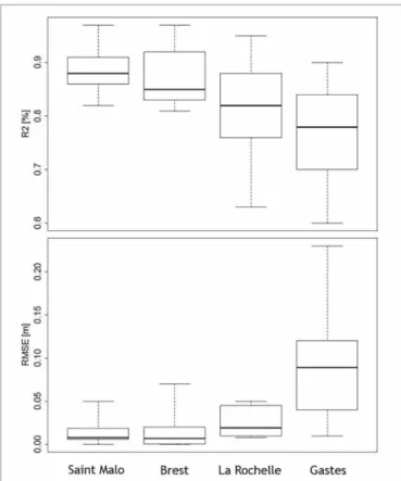
FIGURE 4 | Cross validation results for the four constructed meta-models.

From a practical point of view, the value of K is typically chosen as a good compromise between the computational times needed for the analysis and its reliability (Hastie et al., 2009). Indeed, there is not, to our knowledge, a well-established methodology allowing identifying the optimum number of folds necessary for cross- validation. In this methodological work, we considered K =10 as a robust value with regards to the objectives of the study.

Results in terms of the criteria of quality L are reported in Table 5 and Figure 4. It appears that the mean computed values from cross validation are satisfying when considering the large range of parameters variations of the design data-base and the methodological purpose of the study. Indeed, except for the “Gastes” gauge, the mean R2 is higher than 80%, which is satisfying according to Marrel et al. (2009) and Storlie et al. (2009), and the mean RMSE of few centimeters, indicating that the kriging meta-model is a good emulator choice for reproducing the CEA-tsunami code behavior.

However, it must be underlined that, out of four gauges, results obtained for “Gastes” gauge are not satisfying, at least in terms of statistical performance. In fact, the large variation of the RMSE parameter (from 0.03 to 0.25 m) and the low values of R2 (varying from 0.6 to 0.9) reported in Figure 4 suggest that further numerical runs should be necessary to improve the accuracy of kriging.

It must be noted that the methodology used for the meta- model validation is a “state of the art” methodology permitting to focus on the ability of the meta-model to reproduce the mean model response and to estimate the model variability (represented by the variance). Even if this is common in literature, for hazard studies it would also be of interest to focus in the future on other criteria that account for the behavior in the tails of the distributions of the simulated values (extreme values).

Validation With Results From Allgeyer

et al. (2013)

We perform an additional test in order to evaluate the ability of our meta-models to reproduce state of the art tsunami scenarios generated by the AGPB and impacting the French coast. With this aim, we compare our meta-models results with tsunami height simulated at the same location by Allgeyer et al. (2013). This comparison is of interest in order to confirm the ability of the constructed meta-models to reproduce the order of magnitude of the modeled tsunami height at a given location.

In this study, the authors analyzed the impact of a Lisbon- like tsunami on the French Atlantic Coast through numerical modeling. The authors focused on the simulated maximum tsunami water height in the North Atlantic associated to three different sources for the 1755 events derived from Johnston (1996), Baptista et al. (2003), and Gutscher et al. (2006), for a total of five tsunami scenarios (see Table 6). The same scenarios were simulated with the constructed meta-models for the four French Atlantic Gauges and with the CEA-tsunami model with a more refined grid, spacing of 1'. Even if meta-models prediction slightly overestimate the modeled tsunami height (see Figure 5 and Table 7), these results indicate a good agreement between the meta-modeled and the modeled water height, for the “Saint Malo,” “Brest” and “La Rochelle” gauges. On the contrary, these results confirm that further numerical runs should be necessary to improve the accuracy of kriging for “Gastes” gauge, which largely overestimate the tsunami heights of the original model (Figure 5).

Considering the methodological purpose of the study, these results are satisfying. However, for a practical application, a more extended set of physical scenarios should be of interest for the validation of the tsunami height predicted by meta-models.

POTENTIAL APPLICATION OF

META-MODELS FOR TSUNAMI HAZARD

ANALYSIS

The objective of this section is to present how meta-models can be employed for (i) the integration of uncertainties of “known”

TABLE 6 | Seismic sources simulated in Allgeyer et al. (2013) for the 1755 Lisbon-tsunami.

Hypothesis reported in Allgeyer et al. (2013)

Source _{Strike [0] Length [km]} Dip [0] _{Rake [0]} Width [km] _{Slip [m] Lon [0] Lat [0]} Depth [km]

Johnston, 1996 60 200 40 90 80 13.1 11.45 36.95 27 Baptista et al., 2003 250 155 45 90 55 20 -8.7 36.1 20.5 Gutscher et al., 2006 _{21.7 96 24 90 55 20 -10 36.8 20.5}

346 180 5 90 197 20 -7.5 35.5 15.1

346 180 30 90 12 20 -8.6 35.3 3.2

TABLE 7 | Maximum tsunamis height simulated in Allgeyer et al. (2013) for the 1755 Lisbon-tsunami and computed with meta-models.

Numerical simulations from Allgeyer et al. (2013) Results from meta-models constructed in this study

Source Saint Malo [m] Brest [m] La Rochelle [m] Gastes [m] Saint Malo [m] Brest [m] La Rochelle [m] Gastes [m] Johnston, 1996 0.22 0.54 0.34 0.08 0.28 0.61 0.41 0.3 Baptista et al., 2003 0.06 0.24 0.12 0.02 0.1 0.28 0.2 0.18 Gutscher et al., 2006 0.14 0.35 0.16 0.03 0.18 0.34 0.18 0.18

0.12 0.41 0.2 0.05 0.15 0.45 0.2 0.3

tsunami scénarios (see section “In the case of expert opinion: uncertainty quantification in DTHA”) and (ii) the analysis of the tsunamigenic potential of a poorly known tsunamigenic area (see section “Without expert opinion: exploration of a large tsunamigenic area”). Finally, the obtained results are discussed in light of the tsunami hazard issued by a probabilistic analysis (see section “Qualifying these approaches with respect to Probabilistic Tsunami Hazard Assessment”).

We recall here that this is not an operational tsunami hazard assessment and that all the presented results are purely methodological.

In the Case of Expert Opinion:

Uncertainty Quantification in DTHA

DTHA is classically assessed by means of considering particular source scenarios (usually maximum credible scenario) and the associated maximum tsunami height is generally retained as hazard level (MCS). A more sophisticated method was recently proposed by Roshan et al. (2016). The authors tested around 300 tsunamis scenarios in a [8 - 9.5] magnitude range associated with various faults potentiallyimpactingthe Indian coast. Finally, the authors suggested that an appropriate water level for hazard assessment (e.g., mean value or mean plus sigma value) should be retained. They proposed the mean value of the simulated water heights, as test, by considering that this value may need to be revisited in the future.

In the case of the tsunamis hazard associated with the AGPB, the 1755 Lisbon tsunami is the classical reference scenario. In order to illustrate how to integrate the evaluation of uncertainties in a MCS approach, we focus on two specific and nearly deterministic scenarios considered as likely sources generating the Lisbon 1755 tsunami, namely the Gorringe and Horseshoe structures (Buforn et al., 1988; Stich et al., 2007; Cunha et al., 2012; Duarte et al., 2013; Grevemeyer et al., 2017). Both structures were modeled taking into account available maps (Cunha et al., 2012; Duarte et al., 2013) and fault parameters (Stich et al., 2007; Grevemeyer et al., 2017) summarized in Table 2. For the computation of the tsunami heights associated with these scenarios, fault parameters are considered uniformly distributed and are randomly sampled in their range of variation (Table 2), for a total of nearly 10,000 tsunami scenarios. The magnitude range associated with the sources of these tsunami scenarios varies from 7.7 to 8.9, which is coherent with the range of estimated magnitudes for the 1755 earthquake (Johnston, 1996; Gutscher et al., 2006). The convergence of statistics (defined as the evolution of the mean modeled tsunami height and of the mobile standard deviation) is largely achieved, indicating that the number of tsunami scenarios is sufficient to represent the expected variability of tsunamis height.

The distribution of tsunami heights resulting from the two Gorringe and Horseshoe sources are reported in Figure 6 for each gauge and a summary of the numerical values in Table 8. It can be observed that the tsunami heights generated by the Horseshoe sources are globally lower than those generated by the Gorringe sources. At first glance, this result does not seem surprising considering the closer proximity of the French gauges

to the Gorringe bank. It can also be observed that both scenarios are affected by strong uncertainties. Indeed, the ratio between the maximum and the mean tsunami height is very large and it can vary from 2 to 5, according to the chosen gauges. Moreover, the variability of the modeled values around the mean value can be higher than 1.0 m for the Gorringe scenarios and it is always higher than 0.24 m (for Saint Malo gauge).

If we assume that the MCS approach is to take into account the worst possible scenarios, a hazard level corresponding to the maximum modeled water height could be retained for each gauge. However, if we consider the excursion of our numerical results this hazard level could be too high. This is probably why, as previously mentioned, other authors proposed to set a mean level as representative of the tsunami hazard (Roshan et al., 2016). In general, a first methodological conclusion is that the impact of the uncertainty on the source parameters on water height can be high and it should be taken into account by decision makers.

Without Expert Opinion: Exploration of a

Large Tsunamigenic Area

Let’s now assume, for a methodological purpose, that AGPB is a poorly known seismic area and that the objective of the study are to (i) evaluate the “possible” impact of tsunamis generated by this area on a target location (in this example, the French gauges) and (ii) to better understand the relative influence of the source parameters on these tsunamis. This latter analysis should permit to better guide the geological investigations in the area.

With this objective, UQ and GSA appear as two useful and complementary tools, respectively to answer to objectives (i) and (ii).

Analysis of the Impact of Tsunamis on a Target Area Through UQ

We propose to evaluate the tsunami hazard level, called here MCS_h, by exploring meta-models results based on a very wide range of tsunamigenic scenarios, beyond those proposed so far in the literature as we suppose that this tsunamigenic area is not well known. As a consequence, we accept that through this approach we explore the effects of both likely and very unlikely scenarios relative to the MCS (the “MCS_h” scenarios) that could potentially arise in a context of poor seismotectonic knowledge. As in the previous case, depending on the specific hazard target (civil or industrial facilities), and its location with respect to the source zone, the end-user of this methodology needs to decide which level of water height to choose from the obtained distribution. In this exercise, we will consider the maximum simulated water height for MCS_h.

We build a database (called global database) of tsunami scenario generated by the considered AGPB area at four French Atlantic Gauges, with the aim to cover a wider range of tsunamigenic scenarios (Table 2). For the purpose of this methodological paper, the modeled area, which encompasses different seismotectonic domains, was split in a very simplistic way into two main seismic source zones (Figure 3): a western domain where normal to transtensive earthquakes occur within a thin crust and an eastern domain where reverse to transpressive earthquakes mainly occur on a thicker crust. We considered the

Global Database - MCS Gorringe - MCS HorseShoe - MCS <D

0

Tsunami water height [ml

FIGURE 6 | Tsunami height frequency distribution associated to the global data base (gray-blue), the Gorringe bank (blue) and the Horseshoe bank (green). The black and red lines correspond, respectively, to the mean tsunami height associated to a return period of 1 000 and 10 000 years issued by TSUMAPS-NEAM research project. Dotted lines represent the 2th and 98th percentile of the hazard curves.

TABLE 8 | Maximum tsunami height distributions associated with the global database (GD), HorseShoe (HS), and Gorringe (GR) scenarios; fim, and Maxm correspond to the mean, standard-deviation and maximum meta-modeled values.

Scenarios

Saint Malo Brest La Rochelle Gastes

GD HS GR GD HS GR GD HS GR GD HS GR Minm [m] 0.00 0.03 0.05 0.00 0.00 0.00 0.00 0.00 0.00 0.00 0.00 0.00 fim [m] 0.09 0.18 0.25 0.18 0.31 0.53 0.19 0.26 0.32 0.13 0.18 0.29 [m] 0.17 0.24 0.35 0.34 0.49 0.85 0.36 0.43 0.53 0.27 0.33 0.5 + 2om [m] 0.24 0.3 0.46 0.51 0.66 1.17 0.54 0.63 0.74 0.41 0.47 0.7 Maxm [m] 0.77 0.42 0.66 2.01 0.96 1.60 1.81 1.05 1.04 1.92 0.87 1.06

Western domain west of the 10oW meridian and the Eastern domain east of this meridian, coinciding roughly with the base of

the continental slope facing the Portuguese coastline. The main fault characteristics considered to build the tsunami data-base in both eastern and western domains are reported in Table 2, following data contained in Buforn et al. (1988), Molinari and Morelli (2011), Cunha et al. (2012).

The considered seismogenic thickness takes into account the depth of the observed seismicity as well as the fact that part of the upper mantle can potentially be mobilized during major earthquakes: the western domain seismogenic crust is considered to be up to 20 km deep (after Baptista et al., 2017), and up to 60 km for the eastern domain (after Silva et al., 2017). The fault parameters are considered uniformly distributed and are randomly sampled in their range of variation. We finally filtered the resulting database according to an aspect-ratio criterion, allowing the ratio between the length and the width of the faults not to exceed the value of 10, which corresponds to an upper bound of what is observed in nature (Mc Calpin, 2009). The final global database contains nearly 50,000 tsunami scenarios, resulting in earthquake magnitudes varying from 6.7 to 9.3 (Table 2), depending on the explored earthquake source characteristics and calculated from Eq 1. This range of magnitudes is consistent with the magnitude range of the design database.

The tsunami water heights distributions associated to the four gauges are reported in Table 8 and Figure 6. As for the previous paragraph, these results show a very large variability in tsunamis height, which is not surprising considering the large range of variation of the source parameters. However, if we compare these results with those obtained in the previous section, we can also observe that Gorringe and Horseshoe banks are among the major contributors to tsunami hazard along the French Atlantic Coast, generated by seismic sources in the AGPB. Indeed, Figure 6 clearly shows that even if some isolated tsunami scenarios can generate a hazard level higher than the Gorringe Scenarios, globally, these sources are representative of the higher tsunamis from the global data-base.

Global Analysis of Seismic Source Influence on the Target Area

A sensitivity analysis is hereafter performed in order to decipher the relative influence of the seismic source parameters. Homma and Saltelli (1996) introduced the total sensitivity index which measures the influence of a variable jointly with all its

interactions. If the total sensitivity index of a variable is zero, this variable can be removed because neither the variable nor its interactions at any order have an influence on the results. This statistical index (called Sobol index “ST” in this paper) is here of particular interest in order to highlight the earthquake source parameters that mostly control the tsunamis height at each tested gauge. In Figure 7, we reported the total Sobol index for the four meta-models of the French Atlantic Gauges computed with the methodology proposed by Jansen et al. (1994) using the sensitivity-package R (Pujol et al., 2017). The accuracy of Sobol indices performed with Jansen’s method depends on the number of model evaluations. For instance, in this study, we performed nearly 20 000 simulations using meta-models. Results show that the slip parameter is globally the most-influencing parameter for all the French Atlantic Gauges meta-models. Concretely, nearly 50% of the variance of the tsunami water height (the uncertainty) could be reduced by a better knowledge of this parameter. This result is quite obvious considering that the fault- slip directly conditions the ocean floor deformation and hence the tsunami amplitude.

However, this analysis also suggests that the most influencing parameters for the four gauges are slightly different, depending on their location. One can differentiate results obtained for the southern gauges (i.e., La Rochelle and Gastes) from those obtained at northern gauges (i.e., Saint Malo and Brest):

• For the southern gauges, width is the second most relevant parameter, especially at La Rochelle where it is almost as important as the slip parameter. Other important parameters are length and rake, suggesting that for these gauges, fault source parameters in terms of magnitudes (depending on width, slip and length according to equations 1 and 2) and kinematics are the most important in generating hazard;

• For the northern gauges, apart from slip, strike, width and rake are also important, but slightly less than the longitude parameter. This means that the location ofthe source is here of major importance. A possible physical reason could be associated to the lack of the natural barrier composed by the north of Spain and Portugal which protects southern gauges from AGPB related tsunamis compared to northern gauges. As a consequence, the northern gauges should be more exposed to hazard in comparison to southern gauges, located in the shadow of Portugal and Spain.

dip strike lat rake Ion depth length width slip dip lat Ion depth strike length rake width slip

FIGURE 7 | Total order Sobol Index computed forthe French Atlantic Gauges.

Qualifying These Approaches With

Respect to Probabilistic Tsunami Hazard

Assessment

Let’s imagine now that for the target area a reference hazard level is provided through a probabilistic study and that we aim to qualify the robustness of this hazard level with regards to possible tsunamis height issued by expert scenarios (MCS, see section “In the case of expert opinion: uncertainty quantification in DTHA”) or by the exploration of poorly known tsunamigenic area (MCS_h, see section “Without expert opinion: exploration of a large tsunamigenic area”). The idea is here to compare the results from a probabilistic analysis with the deterministic approach proposed in this study, which should permit to completely cover the uncertainty related to seismic source parameters.

With this aim, we compare our results to the tsunami hazard level (Figure 6) issued from TSUMAPS-NEAM research project4 in four points located near to the gauges used in this study. TSUMAPS-NEAM results are provided in terms of Maximum Inundation Height (MIH), which is the estimated maximum flow depth from the envelope of the tsunami wave at all times, as reported in the NEAMTHM18 documentation (Basili et al., 2018, 2019). TSUMAPS-NEAM has developed a long-term PTHA for

4http://www.tsumaps-neam.eu/

earthquake-induced tsunamis for the coastlines of the NEAM region (NE Atlantic, the Mediterranean, and connected seas). TSUMAPS-NEAM results largely relied on inputs from the EU FP7 project ASTARTE, of the GAR15 (global risk quantification under the HFA), and national PTHAs like those of USA and Italy. One of the major results of the project is the Interactive Hazard Curve Tool5 which represents online hazard maps for different hazard probability/average return periods (mean, median, 2nd, 16th, 84th, and 98th percentiles hazard curves). In TSUMAPS- NEAM, tsunamis are computed using an approach which relies on the use of unit sources to reproduce tsunami scenarios (e.g., Molinari et al., 2016; Baptista et al., 2017). The main differences with our methodology are that these methods rely on a decomposition of the tsunami waves form recorded in a target area with simplified methods (e.g., the Green’s law), and on the main assumption that the non-linear terms of tsunami propagation are negligible. The scope of these studies is to develop a fast emulator, permitting to replace a tsunami model at some selected locations, along the same philosophy of the meta-models developed here. As a consequence, according to the author’s purpose, MIH is suitable for a regional, initial screening assessment type such as the objective of TSUMAPS-NEAM. These results must be considered only as input reference study for 5http://ai2lab.org/tsumapsneam/interactive-hazard-curve-tool/

further site-specific assessment. Considering the methodological objective of this work, it is of interest to compare our results with this previous work.

For this exercise, we selected two targets return periods of 1,000 and 10,000 years from the hazard curves of TSUMAPS- NEAM. To take into account the uncertainty related to these results, we consider the mean, the 2th and the 98th percentile hazard curves. These targets, and the associated uncertainty, are typical of classical risk analysis and permit to compare the distributions issued by PTHA with our results. For instance, after the Fukushima accident, a return period of 10,000 years is considered as the target for hazard assessment in the field of nuclear safety (WENRA, 2015).

Figure 6 illustrates the comparison of our results (MCS and MCS_h) with those selected from the TSUMAPS-NEAM project. One can notice that:

• The tsunami intensity associated to a target mean return period of 1,000 years does not cover the tsunamis intensities related to expert scenarios (Gorringe and Horseshoe banks) or to MCS_h scenarios (all the likely and unlikely scenarios from AGPB);

• The tsunami intensity associated to a target mean return period of 10,000 years covers all the tsunami intensities related to seismic sources from the AGPB, including very unlikely tsunami scenarios (MCS_h);

• A target hazard level of 10,000 years covers the tsunamis related to Horseshoe banks;

• A target hazard level of 10,000 years covers the tsunamis related to Gorringe bank, with the exception of “Brest” gauge and to some extent that of “Gastes”.

Even if these results are purely methodological, it appears that a target hazard level of 10,000 years issued from TSUMAP- NEAM project covers all the variability related to seismic sources from the AGPB, even by exploring very unlikely tsunami scenarios (MCS_h) and most of the variability related to Gorringe and Horseshoe scenarios. However, concerningthe “Brest” gauge, the methodology indicates a high sensitivity of this coastal area to the characteristics of the Gorringe seismic sources.

DISCUSSION AND CONCLUSION

The research work presented in this paper was performed in order to test the interest of UQ for the analysis and the qualification of the DTHA generated by earthquakes. We propose a new methodology, permitting the assessment of the uncertainty related to tsunami hazard through the analysis of a wide range of tsunami scenarios at a given location. This concept should permit to define a hazard level which goes beyond the definition of the Maximum Credible Scenario (MCS) classically reported in the literature (JSCE, 2002; Lynett et al., 2004) and employed for DTHA and permit to integrate uncertainty in hazard quantification. Moreover, tsunami hazard evaluated through UQ can also permit the exploration of tsunamigenic potential of a poorly known seismic zone, as well as a qualification of PTHA.

From a methodological point of view, meta-models appear as a very efficient and viable solution to the problem of generating many computationally expensive tsunamis simulations. As reported in Behrens and Dias (2015), the statistical emulator gives perfect predictions at the input points that are used in its generation process (it interpolates). Statistical emulation does not accelerate the model itself. The significant advantage of using the emulator is that it is much less computationally demanding to be evaluated and, therefore, it can be employed to carry out fast predictions and inexpensive analyses, such as sensitivity and uncertainty analyses reported in this study. Even if it is the first time, to our knowledge, that meta-models are proposed for THA, they have been already employed for tsunami modeling (Sarri et al., 2012; Sraj et al., 2014; Rohmer et al., 2018). As reported in section “Qualifying these approaches with respect to Probabilistic Tsunami Hazard Assessment,” in the field of tsunami hazard, an alternative approach relies on the use of unit sources to reproduce tsunami scenarios (e.g., Molinari et al., 2016; Baptista et al., 2017). Results from these studies are satisfactory for most of the practical applications such as probabilistic tsunami hazard analysis, tsunami source inversion and tsunami warning systems. However, we consider that our methodology can be proposed as an alternative to these studies as it does not rely on any assumption on tsunami propagation and can be applied everywhere in the model domain, without any limitation. For instance, meta-models could be constructed and validated from detailed simulations in a given target area, including complex physical phenomena as overtopping, run-up, and breaking. However, we want to stress that meta-model construction is time consuming and needs an appropriate design data-base, which requires a good compromise between the range of variations of the inputs and the number of simulations.

Concerning our application at four selected location, with the exception of “Gastes” gauge, both the statistical tests we performed and the comparison with result from Allgeyer et al. (2013) suggest that the meta-models are able to reproduce the tsunamis generated by the AGPB. Thus, the constructed meta- models could be employed in a further study to roughly evaluate the impact of other seismic scenarios from the AGPB and impacting the French Atlantic Coast offshore. In order to increase the accuracy of “Gastes” meta-model, the design data-base should be however enriched.

Results from GSA suggests that beyond earthquake magnitudes, the position and the orientation of the faults are influent parameters, at least for the sites considered along the northern French Atlantic Coast. Indeed, sensitivity analysis can be a useful tool not only to parametrize the design data-base but also to orient future geological surveys in a specific area.

In conclusion, MCS_h in the AGPB study region as defined in our study could be implicitly associated to a mean return period of 10,000, when considering the strong hypothesis we did on source characteristics. In this sense, results from UQ shows that a hazard level of 10,000 years issued from TSUMAP- NEAM project covers a very wide range of uncertainties related to characterization of seismic sources from the AGPB, even by exploring very unlikely tsunami scenarios (MCS_h) and

most of the uncertainties related to Gorringe and Horseshoe banks expert opinion scenarios. However, concerning the “Brest” gauge, even a target hazard level of 10,000 years does not seem appropriate to cover all the uncertainties related to the Gorringe source, indicating a high sensitivity of this coastal area to the characteristics and the kinematics of the Gorringe seismic source.

PERSPECTIVES

For an operational far-field DTHA, it should be necessary, at first, to improve the actual numerical model in order to better represent the tsunamis run-up and the inundated areas, with a more accurate bathymetric grid. For an operational application to locations closer to the source zones (i.e., Portugal or Spain, Morocco), it may be challenging to gather the necessary details for a proper establishment of both models and meta- models. However this point deserves further attention because uncertainties will always remain. Thus even in such cases, where more refined databases need to be established, the proposed approach should be of interest to at least efficiently explore in a more exhaustive way the uncertainties (e.g., different probability distribution of inputs parameters, non-uniform slip distribution, fault geometries) in the source parameters linked to the MCS approach. Moreover, it must be noted that for this methodological study we chose a very simple but widely used source description (planar faults with homogeneous slip). However, more robust simulations should take into account a more complex source representation (e.g., 3D geometry, heterogeneous slip distribution), as recently suggested by Davies and Griffin (2019). Indeed, meta-models may also be useful to account for these parameters, allowing for many simulations.

From a methodological point of view, it could be of interest to compare our methodology with the alternative approaches using unit sources to reproduce tsunami scenarios (e.g., Molinari et al., 2016; Baptista et al., 2017), in terms of simulations needed, computational time, accuracy, for instance.

Finally, from a numerical point of view, it would be of interest to (1) introduce recurrence models for each tsunamigenic source to go toward PTHA calculations, and (2 introduce meta-models

REFERENCES

Abily, M., Bertrand, N., Delestre, O., Gourbesville, P., and Duluc, C.-M. (2016). Spatial Global sensitivity analysis ofhigh resolution classified topographic data use in 2d urban flood modelling. Environ. Model Softw. 77, 183-195. doi: 10.1016/j.envsoft.2015.12.002

Adetula, B. A., and Bokov, P. M. (2012). Computational method for global sensitivity analysis of reactor neutronic parameters. Sci. Technol. Nucl.

Installations 2012:11. doi: 10.1155/2012/109614

Allgeyer, S., Daubord, C., Hébert, H., Loevenbruck, A., Schindelé, F., and Madariaga, R. (2013). Could a 1755-like tsunami reach the french atlantic coastline? Constraints from twentieth century observations and numerical modeling. Pure Appl. Geophys. 170, 1415-1431. doi: 10.1007/s00024-012- 0513-5

Arakawa, A. (1972). Design of the UCLA General Circulation model. In

Numerical Simulation of Weather and Climate. Tech. Rep. No. 7. Los

Angeles, CA.

Bachoc, F. (2013). Cross validation and maximum likelihood estimations of hyper-parameters of gaussian processes with model misspecification.

in systems developed for tsunami early warning, considering the low computational time inherent to this statistical tool.

DATA AVAILABILITY STATEMENT

The datasets generated for this study are available on request to the Institute for Radiological Protection and Nuclear Safety (IRSN).

AUTHOR CONTRIBUTIONS

VB: development of the methodology, meta-models construction and validation, and sensitivity and hazard analysis. HJ and OS: seismic sources definition, and seismological and hazard analysis. EA: tsunamis modeling (model construction and simulations of the design data-base). LB and C-MD: technical discussions. HH: tsunamis modeling and technical discussions. VB, HJ, and OS wrote the manuscript.

FUNDING

This research was funded by the French National Agency for Research (ANR).

ACKNOWLEDGMENTS

This study was performed through a cooperative research between the Institute for Radiological Protection and Nuclear Safety (IRSN) and the CEA, in the framework of the French ANR- TANDEM research project. We want to thank ENS Paris and particularly the Geology Laboratory for their technical support on this project. We acknowledge especially Eric Calais for the availability of a part of the team’s cluster and Pierpaolo Dubernet for the help he offered to install Promethee. The present work also benefited from the inputs of Msc. Hend Jebali and Dr. Audrey Gailler and from the valuable technical assistance of Dr. Maria Lancieri, Dr. Yann Richet, and Miss Ludmila Provost.

Computa. Stati. Data Anal. 66, 55-69. doi: 10.1016/j.csda.2013. 03.016

Baptista, M., Miranda, P., Miranda, J., and Victor, L. M. (1998). Constrains on the source of the 1755 Lisbon tsunami inferred from numerical modelling of historical data on the source of the 1755 Lisbon tsunami. J. Geodyn. 25,159-174. doi: 10.1016/s0264-3707(97)00020-3

Baptista, M. A., Miranda, J. M., Chierici, F., and Zitellini, N. (2003). New study of the 1755 earthquake source based on multi-channel seismic survey data and tsunamimodeling. Nat. HazardsEarth Syst, Sci. 3, 333-340. doi: 10.5194/nhess- 3-333-2003

Baptista, M. A., Miranda, J. M., Matias, L., and Omira, R. (2017). Synthetic tsunami waveform catalogs with kinematic constraints. Nat. Hazards Earth Syst. Sci. 17, 1253-1265. doi: 10.5194/nhess-17-1253-2017

Barkan, R., Uri, S., and Lin, J. (2009). Far field tsunami simulations of the 1755 Lisbon earthquakeImplications for tsunami hazard to the US East Coast and theCaribbean. Mar.Geol.264, 109-122. doi: 10.1016/j.margeo.2008. 10.010

Baroni, G., and Tarantola, S. (2014). A General probabilistic framework for uncertainty and global sensitivity analysis of deterministic models A