HAL Id: hal-02549422
https://hal-pjse.archives-ouvertes.fr/hal-02549422
Preprint submitted on 21 Apr 2020
HAL is a multi-disciplinary open access
archive for the deposit and dissemination of
sci-entific research documents, whether they are
pub-lished or not. The documents may come from
teaching and research institutions in France or
abroad, or from public or private research centers.
L’archive ouverte pluridisciplinaire HAL, est
destinée au dépôt et à la diffusion de documents
scientifiques de niveau recherche, publiés ou non,
émanant des établissements d’enseignement et de
recherche français ou étrangers, des laboratoires
publics ou privés.
The Adverse Effect of Finance on Growth
Maxime Fajeau
To cite this version:
WORKING PAPER N° 2020 – 18
The Adverse Effect of Finance on Growth
Maxime Fajeau
JEL Codes: C52, E44, G1, O11, O16
Maxime Fajeau
April 20, 2020
Abstract Since the global financial crisis of 2008, a strand of the literature has documented a threshold beyond which financial development tends to affect growth adversely. The evidence, however, rests heavily on internal instrument identification strategies, whose reliability has received surprisingly little attention so far in the finance-growth literature. Therefore, the present paper conducts a reappraisal of the non-linear conclusion twofold. First, in light of new data, second, by a thorough assess-ment of the identification strategy. Evidence points out that a series of unaddressed issues affecting the system-gmm setup results in spurious threshold regressions and overfitting of outliers. Simple cross-country analysis still suggests a positive associ-ation for low levels of private credit. However, adequately accounting for country heterogeneity, along with a more contained use of instruments, points to an overall damaging influence of financial development on economic growth. This association is stronger for more recent periods.
Keywords Finance · Growth · Non-linearity · System GMM · Panel Data JEL classification C52 · E44 · G1 · O11 · O16
M. Fajeau
Université Paris 1 Panthéon Sorbonne Paris School of Economics
48 boulevard Jourdan, 75014 Paris E-mail: maxime.fajeau@psemail.eu
acknowledgement – The author thanks Jean-Bernard Chatelain for his support and fruitful dis-cussions, as well as Samuel Ligonnière and seminar participants at Paris School of Economics, the GDR "Money, Bank, Finance" at the Alexandru Ioan Cuza Ias,i University in Romania, the 14th
BiGSEM Workshop at the Bielefeld University in Germany and the 3rd Ermees Macroeconomic Workshop at the Strasbourg University in France for helpful comments and suggestions.
1 Introduction
Financial development as a source of growth has been the subject of renewed interest since the wake of the 2007/8 crisis. A decade after the financial crisis, this paper intends to contribute to the debate in light of new data and advances in econometric techniques.
Is financial development a leading factor for growth, and if so, should we further stimulate its deepening? No straight answer has emerged. The absence of a consensus is already a defining characteristic of the finance-growth literature, notably on the direction of causality.1
The finance-growth literature and the banking crises literature have left many researchers with conflicting and contradictory findings. Up to the financial crisis, the literature has been quite confident regarding the growth-enhancing properties of financial sector’s expansion (King and Levine, 1993; Levine et al, 2000; Rioja and Valev, 2004; Demetriades and Law, 2006). However, considering more recent data, Rousseau and Wachtel (2011) show that the positive relationship between finance and growth is not as strong as it was in previous studies using data prior to 1990. Focusing on an alternative proxy for financial development, Capelle-Blancard and Labonne (2016) show that there is no positive relationship between finance and growth for OECD countries over the past 40 years. Demetriades and Rousseau (2016) also find that financial depth is no longer a significant growth determinant. Together with the evident damaging impact of the financial crisis on subsequent economic growth, these findings have led several studies to reconsider prior conclusions and investigate potential non-linearities.
To provide a convincing reading through these puzzling conclusions, a strand of the literature has investigated whether there is evidence of a threshold in the finance-growth relationship (see, for instance, the contribution of Cecchetti and Kharroubi, 2012; Arcand et al, 2015; Benczur et al, 2019; Swamy and Dharani, 2020). The later studies conclude that financial deepening starts harming output growth when credit to the private sector roughly reaches a certain threshold somewhere around 100% of GDP. In other words, the non-linear conclusion implies that the financial sector can grow too large for society’s benefits. Such a finding has tremendous policy implica-tions. The level of credit to the private sector of most developed economies is often well beyond this estimated limit (see Figure 1). Therefore, a decade of expansionist monetary policy, easing private credit, would prove to be reckless.
Far from gaining the full support of the entire economic community, there are reactions to this unifying reading of the nexus, challenging earlier results. Karagiannis and Kvedaras (2016) find that the non-linear conclusion is no longer present when restricting the panel to the OECD or the EU countries. Such evidence emphasizes that the threshold estimates could be a byproduct of unaccounted heterogeneity. Based on various dynamic threshold estimates, Botev, Égert, and Jawadi (2019) also fail to find a non-linear association between finance and growth. Such evidence further suggests that the threshold estimates are likewise sensitive to the estimation technique.
In line with this inconclusive literature, the present paper seeks to understand why prior evidence relying on large panels led to non-linear conclusions. The present study reassesses the non-linear evidence twofold. Firstly, by using more data. The new dataset results in additional countries and observations. It extends the scope of the study up to 2015, thereby including additional post-crisis observations. Second, in reexamining the non-linear conclusion in its original methodological environment, this study also sets the focus on the soundness of the econometric methodology. The
.2 .3 .4 .5 .6 .7 C re d it t o Pri va te Se ct o r/ G D P 1975 1985 1995 2005 2015 Year Mean Median
Mean and Median Values
0 .1 .2 .3 .4 Sh a re o f o b se rva ti o n s 1975 1985 1995 2005 2015 Year >90% >120% PC/GDP >90% & >120%
Fig. 1 Evolution of the ratio of credit to the private sector over GDP as a proxy of financial depth, based on the new expanded dataset for 140 countries over 1970-2015. The left panel plots the mean and median values of private credit. The right panel plots the share of observations for which private credit is above 90% (solid line) and 120% (dashed line).
finance-growth nexus is no exception to the well known empirical struggle to iden-tify a causal impact. Moving beyond mere statistical association requires the use of instrumental variables in order to extract the exogenous component of financial de-velopment. The recent non-linear finance-growth literature heavily relies on internal instrument identification strategies in the spirit of Arellano and Bond (1991) and Arellano and Bover (1995).2 However, only limited attention is drawn to the
poten-tial fragility of such System GMM identification strategies (for recent examples, see Cheng et al, 2020; Swamy and Dharani, 2020). Following advances in econometric research, this study takes a look under the hood of the System GMM estimator. To do so, it focuses on alternative specifications to avoid the default implementation pitfalls and provides tests to asses the instruments’ strength. This paper discusses the assumptions underlying the validity of the identification strategy, and thereby the reliability of the threshold estimates. This study is, therefore, the first to pro-vide a thorough appraisal of the internal instrument identification strategies in the non-linear finance-growth literature.
This study provides a body of evidence that dismisses the relevance of a thresh-old in the finance-growth nexus. It shows that uncontrolled country-specific factors and a few outliers are driving former hump-shaped conclusions. This paper provides evidence calling into question the soundness of the various identification strategies. It demonstrates that the conclusion of a non-monotonic causal impact of finance on growth relies on a very large number of either irrelevant or weak instruments. These problematic instruments prevent reliable causal inferences about the effect of finan-cial depth on growth. Further evidence suggests that the near-multicollinearity of the financial proxies, combined with the weak instrument proliferation issue, fosters spurious regressions overfitting a few outliers.
2 The influential contribution of La Porta et al (1997, 1998) suggested the predetermined legal origin of a country as an external instrument for identifying the causal impact of finance on growth. The "legal origin" instrument, while widely used for a time, has been recast by Bazzi and Clemens (2013) because its widespread use to instrument a variety of endogenous variables could only lead to valid instrumentation in at most one of the study. And at worst none.
Finally, this study further contributes to the literature by establishing an overall negative relationship running from financial depth to growth, with a stronger empha-sis in recent periods. These empirical findings support the hypotheempha-sis that financial deepening has done more harm than good in the long run. This conclusion is in line with recent studies providing similar evidence (Cournede and Denk, 2015; Cecchetti and Kharroubi, 2015; Karagiannis and Kvedaras, 2016; Demetriades et al, 2017; Cheng et al, 2020).
The paper proceeds as follows. Section 2 overviews data and methodology. Sec-tion 3 provides some preliminary comments on cross-country regressions. The paper delves into a complete reappraisal of the threshold estimates based on panel data esti-mates in section 4. Then, section 5 provides alternative estiesti-mates unveiling a damaging impact of financial deepening. Finally, section 6 concludes this study.
2 Data and Methodology
2.1 Data and variables
The dataset is gathered from the usual sources. Throughout the study, the indepen-dent variable is economic growth, measured as the log-difference of real GDP per capita (WDI, World Bank, 2018). The proxy used to measure financial development is common to the finance-growth literature: credit to the private sector by deposit money banks and other financial institutions as a ratio of GDP. This variable is pro-vided and actualized by Beck et al (2000a) and Cihak et al (2012).
All regressions are conducted with a set of control variables common to growth empiric literature: the logarithm of initial GDP per capita, average years of education (Barro and Lee, 2013), a measure of trade openness (computed as exports plus imports divided by GDP), and two measures of macroeconomic stabilization, the log of the inflation rate and the log of government consumption normalized by GDP (gathered from WDI, World Bank, 2018).
For comparison purposes with existing literature, this study also works with an older dataset gathered from Arcand et al (2015). This older dataset ranges from 1960 to 2010. Besides extending the sample length, it is worth noting that the new dataset does not exactly match the former. There are inevitable data revisions, where some values are reclassified as missing, and some become available. The correlations, however, are usually close to 0.98 within the sample (including the proxy for financial depth), except for the government consumption ratio, which is 0.94.
The new dataset results in additional countries and observations. It extends the scope of the study up to 2015, thereby including additional post-crisis observations. The paper focuses on the most extended period range. Indeed, one of the alleged strength of the non-linear estimates is to remain statistically significant in long sam-ples where other linear specifications fail to find a significant association between finance and growth. The number of countries varies slightly depending on data avail-ability and is always displayed in the tables containing the results.
2.2 Empirical Methodology
This study aims to reassess the finance-growth relationship, with a particular focus on the non-linear finding in its original methodological environment. A host of em-pirical papers have found evidence of a threshold in the finance-growth relationship. From a methodological perspective, they boil down to dynamic panel data estimates
based on System GMM estimator using five-year periods to smooth out business cycle (Cecchetti and Kharroubi, 2012; Arcand et al, 2015; Sahay et al, 2015; Benczur et al, 2019; Cheng et al, 2020).
The standard estimated model proceeds as follows. Define the logarithmic growth in real GDP per capita for country i between t and t + k as:
∆yi,t+k= 1 k k X j=1 (yi,t+j− yi,t−1+j) (1)
which translates into the average annual growth rate of per capita GDP. For a five-year spell, i.e. k = 5, equation (1) simplifies as:
∆yi,t+5=
1
5(yi,t+5− yi,t)
Let’s denote yi,t as the initial level of log GDP per capita, and yi∗ the long-run (or
steady-state) value. Generic forms of growth estimation equation are usually obtained from a first-order approximation of the neoclassical growth model (Mankiw, 1995), such that one can derive:
∆yi,t+k= λ (yi,t− y∗i)
where λ is the classical conditional convergence parameter. Generally, for practical purposes, the literature implicitly assumes that yi∗can be modeled as a linear function of several variables that impact the structure of the economy (Bekaert et al, 2005). The government’s spending, inflation, average years of secondary schooling, and many other control variables enter the empirical growth studies on this account. The esti-mated growth model, non-linear and non-monotonic with respect to financial depth, has the following form:
∆yi,t+k= λyi,t+ β1P Ci,t+ β2P Ci,t2 + γxi,t+ νit+k (2)
νit+k = µi+ λt+k+ εi,t+k
where the subscripts i and t refer to cross-section unit and time period. P Ci,t is the
ratio of private credit over GDP used as a proxy for financial development. xi,tis the
set of control variables. Finally, νit follows a two-way error component model where
µi, λt and εi,t are respectively the country-specific effect, the period-specific effect
and the error term. The inclusion of time dummies allows capturing period-specific effects, proxying for world economic conditions.
The non-linear and non-monotonic estimations are based on a linear term for private credit, augmented with its quadratic counterpart. The method proposed by Sasabuchi (1980) and developed by Lind and Mehlum (2011), henceforth SLM test, is suited to ascertain the location and relevance of the extremum point. It involves determining whether the marginal effect of finance on growth is significantly different from zero and positive at a low level of finance but negative at a high level, within-sample:
H0: (β1+ 2β2P Cmin≤ 0) ∪ (β1+ 2β2P Cmax≥ 0) i.e monotone or U-shaped
H1: (β1+ 2β2P Cmin> 0) ∪ (β1+ 2β2P Cmax< 0) i.e inverted U-shaped.
The estimation method relies on dynamic panel System GMM estimator, intro-duced by Arellano and Bover (1995) and Blundell and Bond (1998). This GMM inference method has been applied extensively in economic growth and finance litera-ture. It improves upon pure cross-country work in several respects. First, it deals with the dynamic component of the regression specification. It also fully controls for un-observed time- and country-specific effects. Finally, it accounts for some endogeneity in the variables, thereby allowing for a causal interpretation of the results.
Table 1 Cross-country OLS Between regressions
(1) (2) (3) (4)
Data Old New New New
Period 1970-2010 1970-2015 1970-2015 1970-2015
Specificity – – w/o 3 obs. strict OLS-BE
Private Credit 5.608*** 4.908*** 4.240 4.244** (1.738) (1.627) (2.871) (1.701) (Private Credit)2 -3.202*** -2.432** -1.751 -1.770* (1.075) (1.048) (2.591) (0.897) Log(init. GDP/capita) -0.611*** -0.752*** -0.716*** -0.735*** (0.173) (0.152) (0.156) (0.161) Log(school) 1.314** 1.460*** 1.465*** 1.370*** (0.501) (0.362) (0.361) (0.370) Log(inflation) -0.165 0.003 -0.005 0.022 (0.139) (0.153) (0.146) (0.250) Log(trade) -0.017 0.224 0.249 0.195 (0.257) (0.267) (0.270) (0.262) Log(gov. cons.) -0.796 -0.865 -1.032* -0.700 (0.519) (0.559) (0.568) (0.543) Observations 64 74 71 74 R2 0.41 0.49 0.50 0.44 dGrowth/dPC=0 86%** 100%* 121% 120% 90% Fieller CI [74%–111%] [81%–181%] [70%–∞] [91%–308%] SLM (p-value) 0.02 0.08 0.41 0.18
Notes: This table reports the results of a set of cross-country OLS Between regressions in which the dependent variable is the average real GDP per capita growth rate. While the first column provides a benchmark of the typical non-linear result from the old dataset, the subsequent columns report various exercises based on the new data set expanding the period and country coverage. Column (2) presents a reassessment. Column (3) excludes CHE, JPN, and USA. Column (4) incorporates a slight methodological correction. The SLM test provides p-value for the relevance of the estimated threshold. Robust Windmeijer
standard errors in parentheses.∗∗∗p < 0.01,∗∗p < 0.05,∗p < 0.10.
3 Preliminary Comments on Cross-country Regressions
3.1 Simple Cross-country Evidence
Before further delving into the panel estimates, this study first focuses on some cross-country evidence. The setup closely follows the econometric methodology of King and Levine (1993) and the early empirical growth literature (see Barro, 1991). Well aware of the various limitations steaming from endogeneity issues, this exercise is only intended as a preliminary reassessment of the threshold estimates. Naturally, panel data comes as serious help to get around many problems cross-sectional regressions fail to address. Therefore, the panel conclusions of the next sections should be viewed as more reliable.
Table 1 reports various cross-country regressions. Column (1) provides a bench-mark based on the old dataset. The point estimate associated with the linear term of private credit is positive, the quadratic term is negative, and both are statistically significant. It indicates that financial depth starts yielding negative returns as credit
ARG AUS AUT BDI BEL BOL BRA CHE CHL CIV CMR COG COL CRI DEU DNK DOM ECU EGY ESP FIN FJI FRA GAB GBR GHA GTM GRC GUY HND
IDNIND IRL
IRN IRQ ISL ISR ITA JAM JPN KEN KOR LKA LUX MAR MEX MLT MYS NER NLD NOR PAK PAN PER PHL PRT PRY RWA SAU SDN SEN SGP SLE SLV SWE SWZ TGO THA TTO TUR URY USA VEN ZAF −4 −2 0 2 4 6 GDP growth 0 .5 1 1.5 2
Credit to Private Sector/GDP OLS estimate
95% CI
Fig. 2 Financial depth and growth using the new expanded data for 1970-2015. The solid black line plots the OLS quadratic fit of column (2), Table 1. The solid light lines are 95% Fieller confidence intervals. The vertical dotted red line marks the threshold estimate at 100%. Point labels are three-letter ISO country codes.
to the private sector reaches 86% of GDP. The reliability of this turning point, how-ever, rests solely on the SLM test. With a low p-value of 0.02, the threshold is well identified.
Now focusing on the new dataset.3 Using additional available countries and
ex-tending the coverage up to 2015, the non-linear finding weakens. The threshold for private credit rises to 100% of GDP with a higher p-value of 0.08 for the SLM test. However, 96% of total observations are below this threshold. Only three countries experience a level of financial depth above the 100% of GDP threshold. None of them reach the 180% threshold above which the marginal effect of financial depth would become both negative and statistically significant.
Figure 2 plots the quadratic fit between financial depth and growth using the new expanded data. It shows that the curvature is due to only three countries above the threshold, namely: the United-States (USA), Japan (JPN), and Switzerland (CHE). The latter has a high private credit-to-GDP ratio because of the credit extended abroad by the two multinational banks UBS and Crédit Suisse, which do not directly finance the Swiss economy.
Column (3) of Table 1 performs the same regression, this time without these three peculiar observations.4As expected, the linear and quadratic terms for private credit
turn insignificant, and the SLM test indicates that the threshold estimate is no longer statistically relevant. The regression in column (3) emphasizes the dependency of the non-linear conclusion over a long period on a few observations driving the results.
3 The coefficient of correlation for the between dimension of private credit with growth is ρ(P C, GR) = 0.27, for the square of private credit with growth ρ(P C2, GR) = 0.19 and for both private credit terms ρ(P C, P C2) = 0.95. Except ρ(P C2, GR), each of them reject the null hypothesis H0: ρ = 0 at the 10% level for N = 74 observations.
4 Both Japan (JPN) and Switzerland (CHE) display high Dfbeta statistics (Belsley et al, 1980). However, as the Dfbeta statistic works by dropping one observation at a time, the United-States (USA) does not display an outstanding statistic as it is caught between the other two observations. The Dfbeta statistic fails to grasp multiple outliers at once.
Performing the regression without the quadratic term leads to a positive and sta-tistically significant coefficient for the variable private credit.5 In the same spirit, a linear spline regression allowing for different slopes when credit to the private sec-tor is above and below 100% of GDP leads to similar conclusions. Financial depth is positively and significantly associated with economic growth when credit to the private sector is below 100% of GDP, and that it is not significantly correlated above this threshold.6 Over a long period, the threshold estimation rests solely on three
observations.
Finally, these estimates raise a methodological question. Strictly speaking, such cross-sectional regressions, focusing only on the permanent differences in mean levels between countries, corresponding to the "between" dimension, would impose a specific data processing. Columns (1) to (3) follow previous work and handle the data by computing the log and square of the average values of the variables before estimating with OLS. However, for the "between" and "within" dimensions to be orthogonal, one would have to work with the average of the logs and squares and not the opposite. Column (4) provides estimates with this methodological correction. This "rigorous" cross-country dimension leads to a much higher threshold for private credit at 120% of GDP. Thus, the SLM test now rejects the presence of an inverted U-shape.
These new estimates reduce the confidence one can have in the conclusion that financial depth is detrimental to economic growth when credit to the private sector reaches 100% of GDP. Moreover, the conclusions drawn from cross-country regressions ignore within-country variation, and country-specific characteristics are most likely driving the results.
3.2 Misleading Identification Through Heteroscedasticity
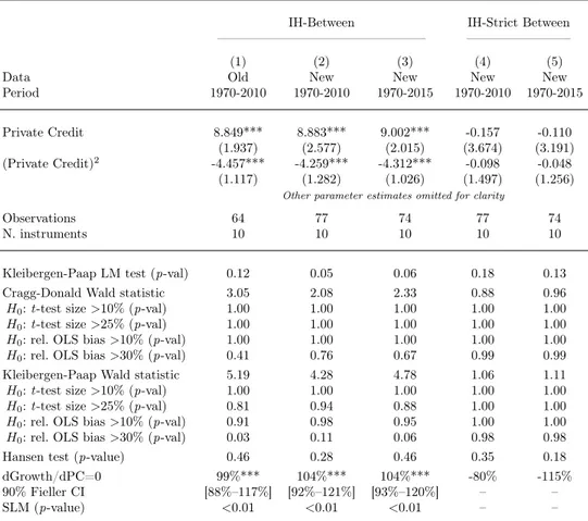
To address the causality issue in these pure cross-sectional country-level regressions, one can use the IV estimator developed by Rigobon (2003) and Lewbel (2012), which relies on heteroscedasticity-constructed internal instruments (henceforth IH). It allows circumventing the lack of suited external instruments. The downside, as emphasized by Lewbel (2012, p.2), is that "the resulting identification is based on higher moments, and so is likely to provide less reliable estimates than identification based on standard exclusion restrictions." Moreover, concern regarding potential weak instruments is real and does not boil down to a question of precision but rather of reliability. Precise estimates convey absolutely no information regarding their reliability. Therefore, weak instruments should be tested for. Thus, Table 2 performs the same regressions as in Table 1, starting with a benchmark threshold estimate from the old dataset, then with the new dataset up to 2010 and 2015. For each specification, Table 2 complements the estimates with tests for underidentification and weak instruments.
For the underidentification, Table 2 reports the p-values for the Kleibergen and Paap (2006) heteroscedasticity robust version of the Lagrange-Multiplier (LM) test. The null hypothesis is that the structural equation is underidentified. A rejection of the null indicates that the smallest canonical correlation between the endogenous variables and the instruments is nonzero. Since the nonzero correlation condition is not enough, Table 2 also controls for weak-instruments by reporting the weak-instruments Wald statistics based on Cragg and Donald (1993), and its non-iid robust analog by Kleibergen and Paap (2006). The latter is better suited due to
heteroscedasticity-5 The coefficient associated with private credit is 1.42 with a p-value of 0.02.
6 Below 100% of GDP, the coefficient associated with private credit is 2.30 with a p-value of 0.003. Above, the coefficient drops to 0.33 with a p-value of 0.55.
Table 2 Misleading cross-country IH regressions
IH-Between IH-Strict Between –––––––––––––––––––––––––––––––– ––––––––––––––––
(1) (2) (3) (4) (5)
Data Old New New New New
Period 1970-2010 1970-2010 1970-2015 1970-2010 1970-2015 Private Credit 8.849*** 8.883*** 9.002*** -0.157 -0.110
(1.937) (2.577) (2.015) (3.674) (3.191) (Private Credit)2 -4.457*** -4.259*** -4.312*** -0.098 -0.048
(1.117) (1.282) (1.026) (1.497) (1.256)
Other parameter estimates omitted for clarity
Observations 64 77 74 77 74
N. instruments 10 10 10 10 10
Kleibergen-Paap LM test (p-val) 0.12 0.05 0.06 0.18 0.13 Cragg-Donald Wald statistic 3.05 2.08 2.33 0.88 0.96 H0: t -test size >10% (p-val) 1.00 1.00 1.00 1.00 1.00 H0: t -test size >25% (p-val) 1.00 1.00 1.00 1.00 1.00 H0: rel. OLS bias >10% (p-val) 1.00 1.00 1.00 1.00 1.00 H0: rel. OLS bias >30% (p-val) 0.41 0.76 0.67 0.99 0.99 Kleibergen-Paap Wald statistic 5.19 4.28 4.78 1.06 1.11 H0: t -test size >10% (p-val) 1.00 1.00 1.00 1.00 1.00 H0: t -test size >25% (p-val) 0.81 0.94 0.88 1.00 1.00 H0: rel. OLS bias >10% (p-val) 0.91 0.98 0.95 1.00 1.00 H0: rel. OLS bias >30% (p-val) 0.03 0.11 0.06 0.98 0.98 Hansen test (p-value) 0.46 0.28 0.46 0.35 0.18 dGrowth/dPC=0 99%*** 104%*** 104%*** -80% -115% 90% Fieller CI [88%–117%] [92%–121%] [93%–120%] – – SLM (p-value) <0.01 <0.01 <0.01 – –
Notes: This table reports the results of a set of cross-country IV regressions in which the dependent variable is the average real GDP per capita growth rate. The identification strategy rests on the estimator developed by Rigobon (2003) and Lewbel (2012), and relies on heteroscedasticity-constructed internal instruments (IH). The following variables are included in the regressions but omitted in the table here for clarity: the logarithm of initial Gross Domestic Product per capita, average years of education, a measure of trade openness, the log of the inflation rate, and the log of government consumption normalized by GDP. While the first column provides a benchmark of the typical non-linear result from the old dataset, the subsequent columns report estimates based on the new dataset expanding the period and country coverage. Column (2) is based on the new dataset with the same time coverage as column (1) but with additional countries. Column (3) expands the coverage up to 2015. Columns (4-5) incorporate a slight methodological correction. The SLM test provides p-value for the relevance of the estimated threshold.
Robust Windmeijer standard errors in parentheses.∗∗∗p < 0.01,∗∗p < 0.05,∗p < 0.10.
robust standard errors. These tests asses whether the instruments jointly explain enough variation to identify unbiased causal effects.
The additional diagnostics proposed by Stock and Yogo (2002) and Yogo (2004) complement these tests: p-values for the null hypotheses that the bias in the estimates on the endogenous variable is greater than 10% or 30% of the OLS bias, and p-values for the null hypotheses that the actual size of the t -test that the coefficient estimates equal zero at the 5% significance level is greater than 15% or 25%.7Finally, the table
reports the Hansen test of overidentifying restrictions, robust to heteroscedasticity.
7 Critical values for the Kleibergen-Paap Wald statistic have not been tabulated, as it depends on the specifics of the iid assumption’s violation. Therefore, following others in the literature (see for more details Baum et al, 2007; Bazzi and Clemens, 2013), the critical values tabulated for the Cragg-Donald statistic are applied to the Kleibergen-Paap statistic.
Columns (1) to (3) of Table 2 show that the coefficients associated with pri-vate credit are precisely estimated, roughly constant for the various regressions, and yield a threshold around 100% of GDP. However, the various specification tests severely reduce the confidence one should have in these results. In column (1), the Kleibergen-Paap LM test of underidenticiation fails to reject the null hypothesis that the structural equation is underidentified. For all regressions, the Cragg-Donald and Kleibergen-Paap Wald-type statistics show that the instrumentation is very weak. Moreover, the high p-values for the various levels of relative OLS bias underlines that the instrumentation is far too weak to remove a substantial portion of OLS bias. Large p-values also indicates that the actual size of the t -test at the 5% level is greater than 25%. The precise estimates are a byproduct of either weak or irrelevant instruments. Column (4) and (5) deal with the methodological issue mentioned in the previous subsection 3.1. They provide estimates with the methodological correction, based on the exact specification of previous columns (2) and (3). This rigorous cross-country dimension leads to insignificant point estimates for the level of private credit and its squared term, along with a negative threshold for private credit. Thus, the SLM test now trivially rejects the presence of an inverted U-shape. The thresholds estimates are highly sensitive to the specific data process.
The IH estimations suffer from weak instrumentation. Thus, not surprisingly, the point estimates from Table 2 are in line with those obtained from the OLS estimator in Table 1. This proximity does not point toward highly causal results. It would rather be a sign of untreated bias and persistent endogeneity. By looking under the hood of the identification through heteroscedasticity, these simple tests shine brighter lights on its inability to yield a reliable identification of a causal impact from finance depth to economic growth.
Panel data comes as serious help to get around many of the problems cross-sectional regressions fail to address. Therefore, the panel conclusions are usually con-sidered as more reliable. Indeed, switching from pure cross-country to panel data mobilizing the time-series dimension has significant advantages. Among them, esti-mates are no longer biased by omitted variables constant over time (the so-called fixed effects). Also, taking advantage of internal instrument techniques allows for consistent estimates of the endogenous models (if carefully and adequately cast).
4 More Reliable Panel Estimates?
4.1 A Very Influential Starting Point
Now turning to a pooled (cross-country and time-series) data set consisting of at most 140 countries and, for each of them, at most 11 non-overlapping five-year periods over 1960-2015.
The five-year spell length is commonly chosen in the literature for several reasons. First, the use of longer periods would significantly reduce the number of degrees of freedom, which is problematic when implementing dynamic panel data procedures. Secondly, five-year periods, as emphasized by Calderon et al (2002), follows the en-dogenous growth literature (e.g. Caselli et al, 1996; Easterly et al, 1997; Benhabib and Spiegel, 2000; Forbes, 2000) where such period length is believed to purge out business-cycle fluctuations which could induce a negative coefficient on private credit. Indeed, the empirical growth literature usually averages out data over five-year spells in order to measure the steady-state relationship between the variables. Smoothing out data series supposedly removes useless variation from the data, enabling precise parameter estimates. Indeed, Loayza and Ranciere (2006) find that short-run surges
Table 3 Sequential anchoring of the five-year spells in dynamic panel regressions (1/2)
(1) (2) (3) (4) (5)
Data Old Old Old Old Old
Coverage 1960-2010 1961-2011 1962-2007 1963-2008 1964-2009 Number of spells 10 10 9 9 9 Private Credit 3.621** 0.171 0.780 0.084 1.971 (1.718) (1.824) (1.877) (1.689) (1.688) (Private Credit)2 -2.018*** -0.882 -0.749 -0.523 -1.418* (0.727) (0.774) (0.889) (0.782) (0.852)
Other parameter estimates omitted for clarity
N. instruments 318 318 254 254 254
N. countries 133 133 134 133 133
Observations 917 916 811 829 858
AR(2) (p-value) 0.11 0.08 0.23 0.51 0.91
Hansen test (p-value) 1.00 1.00 1.00 1.00 1.00
dGrowth/dPC=0 90%** 10% 52% 8% 69%
90% Fieller CI [43%–113%] – – – [0%–124%]
SLM (p-value) 0.03 0.46 0.40 0.48 0.19
Notes: This table reports the results of a set of panel regressions consisting of non-overlapping five-year spells. The dependent variable is the average real GDP per capita growth rate. All regressions contain time fixed effects. The first column reports the best-attempted replication of the typical threshold result from the yearly version of the old dataset. Column (2) provides point estimates with a one-year forward shift for the starting point of each spell. The subsequent columns continue shifting forward by one year the beginning of the five-year spells. The null hypothesis of the AR(2) serial correlation test is that the errors in the first difference regression exhibit no second-order serial correlation. The null hypothesis of the Hansen test is that the instruments fail to identify the same vector of parameters (see Parentes and
Silva, 2012). Robust Windmeijer standard errors in parentheses.∗∗∗p < 0.01,∗∗p < 0.05,∗p < 0.10.
in private credit appear to be a good predictor of both banking crises and slow growth. In the long run, a higher level of private credit is associated with higher economic growth. This tension between short-term and long-term effects justifies the use of low-frequency data to abstract from business-cycles. Finally, this is conveniently suited to the specifics of System GMM, as it requires a short panel characterized by large N and small T dimensions.
The growth variable is usually computed as the average annual growth rate within the five-year spell. All explanatory variables, however, are systematically based on the first observation of each five-year spell. The absence of averaging implies a substantial informational loss as well as a consistency loss. Excluding 80% of the observations would possibly expose the coefficient estimates to bias as it could mismeasure the true explanatory variables. Hence, is the starting point of the five-year spells influencing the results?
Table 3 shows regressions for sequential anchoring of the five-year spells based on the old dataset. Column (1) provides a benchmark (typical) non-linear conclusion. Column (2) provides point estimates with a one-year forward shift for the starting point of each spell, with an identical sample of countries, and one fewer observation (916 against 917 previously) due to data availability. The coefficients associated with the linear and quadratic term of private credit lose magnitude, and neither of them is statistically significant. The SLM test discards the inverted U-shape with a high p-value of 0.46. Through columns (3) to (5), the same exercise goes on by shifting
Table 4 Sequential anchoring of the five-year spells in dynamic panel regressions (2/2)
(1) (2) (3) (4) (5)
Data New New New New New
Coverage 1960-2015 1961-2016 1962-2012 1963-2013 1964-2015 Number of spells 11 11 10 10 10 Private Credit -0.170 2.851* 1.085 0.940 1.027 (1.480) (1.465) (1.408) (1.610) (1.800) (Private Credit)2 -0.256 -1.217* -1.062* -0.901 -0.698 (0.703) (0.699) (0.612) (0.679) (0.721)
Other parameter estimates omitted for clarity
N. instruments 388 388 318 318 318
N. countries 140 140 138 138 138
Observations 1,055 1,085 965 970 987
AR(2) (p-value) 0.40 0.01 0.11 0.56 0.85
Hansen test (p-value) 1.00 1.00 1.00 1.00 1.00
dGrowth/dPC=0 – 117%* 51% 52% 73%
90% Fieller CI – [86%–426%] [0%–95%] – –
SLM (p-value) – 0.06 0.34 0.37 0.33
Notes: This table reports the results of a set of panel regressions consisting of non-overlapping five-year spells. The dependent variable is the average real GDP per capita growth rate. All regressions contain time fixed effects. Each column presents one possible anchoring for the five-year spells in the new dataset. The null hypothesis of the AR(2) serial correlation test is that the errors in the first difference regression exhibit no second-order serial correlation. The null hypothesis of the Hansen test is that the instruments fail to identify the same vector of parameters (see Parentes and Silva, 2012). Robust Windmeijer standard
errors in parentheses.∗∗∗p < 0.01,∗∗p < 0.05,∗p < 0.10.
forward by one year the beginning of the five-year spells. In the end, out of the five possible starting points presented in columns (1-5), only one supports the existence of a threshold.
Table 4 conducts the same exercise, this time based on the new dataset. Each column shifts forward by one year the beginning of the five-year spells. Very similar conclusions arise, as only one estimate out of the five possible anchors supports the presence of a significant threshold. Analogous conclusions are drawn from a restricted sample of the new dataset to match the country coverage of Table 3.
From these various anchoring exercises, a clear recommendation emerges. Averag-ing the explanatory variables within the five-year spell should be favored over initial values, except for the convergence variable8. It is preferable to keep more observations through data averaged over sub-periods, while controlling for endogeneity biases by
8 The work of Caselli et al (1996) is among the first attempts to use the GMM framework to estimate a Solow growth model. They make use of the Barro (1991) method, initially created for cross-sectional data, by adapting it for a panel framework. Already at this early stage, the problem related to extensive use of initial value was raised. They chose to work with the averaged annual growth rate of per capita GDP, but distinguished between state and control variables for the explanatory variables. Controls are averaged over the five-year intervals (government consumption, inflation rate, trade openness). In contrast, only states variables are taken at their initial value (initial level of per capita GDP, the average number of years of schooling). Therefore all variables do not enter with the same treatment.
properly instrumenting the explanatory variables9. Otherwise, coefficient estimates remain exposed to mismeasured true explanatory variables.
4.2 Abundant Weak Instruments
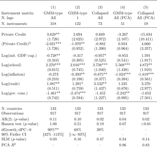
4.2.1 An Instruments Proliferation Issue
The dynamic panel System GMM estimator introduced by Arellano and Bover (1995) and Blundell and Bond (1998) comes in handy to work toward a causal reading of the estimates as no suited external instruments have emerged. However, the default implementation of this estimator generates a set of internal instruments whose num-ber increases particularly quickly with the time dimension of the panel. The dramatic increase (somehow pandemic) in the instrument count is often referred to as instru-ments proliferation. The literature has documented several problems arising with ex-cessive proliferation: overfitting of endogenous variable, weakened Hansen test for over-identifying restrictions, biased two-step variance estimators and imprecise esti-mates of the optimal weighting matrix.10 Fortunately, there are two usual telltale
signs: a number of instruments greater than the number of cross-sectional units (the number of countries), and a perfect Hansen test of 1.00. The non-linear conclusions systematically meet both telltale signs.
Column (1) of Table 5 presents the typical non-linear conclusion based on the old dataset. The coefficient estimates on private credit are significant, and the SLM test corroborates the presence of an inverted U-shape relationship. It indicates that financial depth starts yielding negative returns as credit to the private sector reaches 90% of GDP. However, there are no less than 318 instruments in this default imple-mentation of the System GMM estimator (for only 130 cross-sectional units). Along with the perfect value of 1.00 for the Hansen test, this casts doubts on the reliability of the result, with possible overfitting and failure to expunge the endogenous part as the tests would be weakened in this setup. Moreover, the AR(2) test for autocorre-lation display a p-value of 0.11, which is too low to be considered safe. These tests are conservative, a value close to conventional thresholds should be viewed with a fair degree of caution.
Roodman (2009, p. 156) stresses that "results and specification tests should be aggressively tested for sensitivity to reduction in the number of instruments." The remaining columns of Table 5 present the various instrument count reductions im-plemented as minimally arbitrary robustness checks to examine the behavior of the coefficient estimates and various specification tests.
Column (2) provides the first step of the robustness check strategy to reduce the number of instruments. Alonso-Borrego and Arellano (1999) states that the most distant instruments are generally those which offer the weakest correlation and are therefore the least relevant. Following others in the finance-growth literature, column (2) restricts the instrument matrix to a single lag (see for examples Levine et al, 2000; Beck et al, 2000b; Baltagi et al, 2009; Kose et al, 2009; Law and Singh, 2014). This brings the instruments count down to 122 instruments, below the usual rule of thumbs based on the number of cross-country observations. This time, the coefficient
9 Some papers have taken this path, see for example Benhabib and Spiegel (2000); Beck and Levine (2004); Rioja and Valev (2004); Beck et al (2014b); Law and Singh (2014).
10 For more details, see Andersen and Sorensen (1996); Ziliak (1997); Alonso-Borrego and Arellano (1999); Koenker and Machado (1999); Hayashi (2000); Calderon et al (2002); Bowsher (2002); Alvarez and Arellano (2003); Han and Phillips (2006); Hayakawa (2007); Roodman (2009); Baltagi (2013).
Table 5 Instrument proliferation in System GMM panel regressions for 1960-2010
(1) (2) (3) (4) (5)
Instrument matrix: GMM-type GMM-type Collapsed GMM-type Collapsed
N. lags All 1 All All (PCA) All (PCA)
N. instruments 318 122 73 51 19 Private Credit 3.628** 2.694 0.689 -3.267 -15.834 (1.726) (2.025) (2.972) (2.107) (10.411) (Private Credit)2 -2.021*** -1.970** -0.882 0.924 4.660 (1.726) (0.952) (1.390) (0.964) (3.357) Log(init. GDP/cap.) -0.728** -0.317 -0.957* -0.853 1.591 (0.310) (0.305) (0.525) (0.541) (1.917) Log(school) 2.270*** 2.016*** 3.738*** 5.568*** 4.872** (0.615) (0.745) (1.040) (1.438) (1.910) Log(inflation) -0.273 -0.393** -0.875** -1.024*** -1.819*** (0.210) (0.198) (0.377) (0.394) (0.561) Log(trade) 1.087** 1.291* 3.532** 1.235 3.370 (0.511) (0.759) (1.437) (0.876) (2.977) Log(gov. cons.) -1.461** -2.474*** -1.452 -2.242** -1.652 (0.742) (0.594) (1.227) (0.995) (7.501) N. countries 133 133 133 133 133 Observations 917 917 917 917 917 AR(2) (p-value) 0.11 0.10 0.02 0.04 0.02
Hansen test (p-value) 1.00 0.51 0.19 0.07 <0.01
dGrowth/dPC=0 90%** 68% 39% – –
90% Fieller CI [42%–113%] [-∞–93%] – – –
SLM (p-value) 0.03 0.16 0.47 0.34 0.14
PCA R2 – – – 0.86 0.83
Notes: This table reports the results of a set of panel regressions consisting of ten non-overlapping five-year spells. The dependent variable is the average real GDP per capita growth rate. All regressions contain time fixed effects. While the first column reports a replication of the typical threshold result from the old dataset for 1960-2010, the subsequent columns report various instrument reduction exercises. The null hypothesis of the AR(2) serial correlation test is that the errors in the first difference regression exhibit no second-order serial correlation. The null hypothesis of the Hansen test is that the instruments fail to identify the same vector of parameters (see Parentes and Silva, 2012). The SLM test provides p-value
for the relevance of the estimated threshold. Windmeijer standard errors in parentheses. ∗∗∗p < 0.01,
∗∗p < 0.05,∗p < 0.10.
estimate for private credit in level loses significance, and the SLM test becomes incon-clusive, rejecting the presence of an inverted U-shape. The usual specification tests now systematically reject at lower p-values, displaying a serious sign of second-order autocorrelation. The Hansen test now returns a lower p-value of 0.51, much lower than the initial 1.00.
Collapsing the instrument matrix further reduces the instrument count. Whereas limiting the lag depth still relies on different sets of instruments for each time period, the collapsing works around with moment conditions applied such that each of them corresponds to all available periods (Calderon et al, 2002). It maintains the same amount of information from the original 318 columns instrument matrix, yet com-bined into a smaller set.11 The number of instruments now falls to 73. Column (3)
11 For an application to the finance-growth setup, see the work of Beck and Levine (2004) or Carkovic and Levine (2005).
displays results for this exercise. Both coefficient estimates for private credit in level and squared are no longer significant. Once again, the SLM test rejects the presence of an inverted U-shape between finance and growth. Moreover, the p-value of the AR(2) test now dips down to 0.02, confirming the previously suspected autocorrelation is-sue. The Hansen test’s p-value falls to 0.18, as compared to the 1.00 for the default implementation.
The penultimate technique to reduce the instrument count without either cutting into the lag depth or the GMM-style construction of the instrument matrix is to replace the prolific instruments by their principal components (Kapetanios and Mar-cellino, 2010; Bai and Ng, 2010; Bontempi and Mammi, 2012). Column (4) presents results for this principal components analysis (PCA) technique, which enables to maintain a substantial amount of the information in the instruments into less exten-sive moment conditions. The identification now rests on 51 instruments. The coeffi-cient estimates for private credit are insignificant, and of opposite sign as compared to the default implementation of column (1). Once again, the SLM test confirms the absence of an inverted U-shape. Other coefficients remain roughly in line with the default implementation, with slightly higher absolute values. Both the AR(2) test and Hansen test return very low p-values of 0.04 and 0.07 respectively, discarding the reliability of the results.
Finally, the last column combines PCA and collapse techniques, as Mehrhoff (2009) concludes that PCA performs reasonably well when the instrument matrix is collapsed prior to factorization (see for example Beck et al, 2014a). Column (5) displays this ultimate reduction to 19 instruments. The point estimate and standard errors for private credit are more than four times higher in absolute value than in the baseline regression from column (1). Just as in column (4), private credit and its square term switch signs. The SLM test discards once again the presence of an inverted U-shape. The main specification tests now display extremely low p-values, discarding the ade-quacy of the model: 0.02 and 0.00 for the AR(2) and the Hansen test, respectively.
Overall, there is a substantial and systematic decrease in the p-values of both the Hansen test and the AR(2) test as the number of instruments falls. Given the overall dependence of the non-linear conclusion on a very high instrument count, these straightforward techniques highlight a strong possibility of overfitting and concerns of third-variable or reversed causation. The general dependence of the results on a specific instrument matrix also gives hints toward a weak instrument problem.
4.2.2 Far Too Weak Instruments
A reliable causal inference of financial depth on growth requires the instruments to display a strong relationship with the endogenous explanatory variables. When this relationship is only weak, instrumental variable estimators are severely biased (see for a survey Murray, 2006; Mikusheva, 2013). The System GMM estimator is far from immune to the weak instruments’ problem (Hayakawa, 2009; Bun and Windmeijer, 2010).
Measuring how much of the variation in the endogenous variables is explained by the internal instruments is crucial, and often remains unexplored. Most applications of the System GMM assume that instruments are strong. The issue goes far beyond the finance-growth literature. Indeed, testing for weak instruments is not straightforward in dynamic panel GMM regressions due to the absence of standardized tests.
To circumvent this issue, Bazzi and Clemens (2013) have come up with a simple "2SLS analog" technique. Since weak instrument tests are available within the 2SLS setup, carrying out the equivalent regression using 2SLS with the identical GMM-type
Table 6 Weak instruments in dynamic panel regressions
Difference equation Levels equation ————————– ————————– Estimator GMM-SYS 2SLS 2SLS 2SLS 2SLS Collapsed IV matrix No No Yes No Yes
(1) (2) (3) (4) (5)
Private Credit 3.628** -5.110** 1.380 4.247** 16.220 (1.726) (2.161) (4.020) (2.028) (121.16) (Private Credit)2 -2.021*** 0.536 -2.278 -2.765*** -11.390
(1.726) (0.825) (1.896) (0.996) (81.01)
Other parameter estimates omitted for clarity
Observations 917 780 780 917 917 N. countries 133 130 130 133 133 N. instruments 318 261 57 65 16 IV: Lagged levels Yes Yes Yes No No IV: Lagged differences Yes No No Yes Yes
Kleibergen-Paap LM test (p-value) 0.286 0.465 0.518 0.894 Cragg-Donald Wald statistic 0.89 0.68 0.83 0.002 H0: t -test size > 10% (p-value) 1.000 1.000 1.000 1.000
H0: t -test size > 25% (p-value) 1.000 1.000 1.000 1.000
H0: rel. OLS bias > 10%(p-value) 1.000 1.000 1.000 1.000
H0: rel. OLS bias > 30%(p-value) 1.000 1.000 1.000 0.999
Kleibergen-Paap Wald statistic 3.17 0.85 1.15 0.002 H0: t -test size > 10% (p-value) 1.000 1.000 1.000 1.000
H0: t -test size > 25% (p-value) 1.000 1.000 1.000 1.000
H0: rel. OLS bias > 10% (p-value) 1.000 1.000 1.000 1.000
H0: rel. OLS bias > 30% (p-value) 0.614 1.000 1.000 0.999 Notes: This table reports the results of a set of minimally arbitrary weak instrument test opening the "black box" of the System GMM estimator. The panel regressions are based on ten non-overlapping five-year spells and contain time fixed effects. The dependent variable is the average real GDP per capita growth rate. While the first column simply reproduce the baseline result from the old dataset for 1960-2010 (see Table 5, column (1)), the subsequent columns report the decomposition of the System GMM following
the "2SLS analogs" of Bazzi and Clemens (2013). Windmeijer standard errors in parentheses.∗∗∗p < 0.01,
∗∗p < 0.05,∗p < 0.10.
instrument matrix provides "simple and transparent tests of instrument strength in a closely related setting" (Bazzi and Clemens, 2013, p. 167). This exercise requires to split the System GMM in two: the difference part and the level part.
Table 6 reports point estimates for this exercise along with various specification tests for the typical threshold from the old dataset. Once again, the table displays tests for underidentification (Kleibergen-Paap LM test) and weak instruments (Cragg-Donald and Kleibergen-Paap Wald tests).12
Column (1) provides the benchmark System GMM estimates. Column (2) presents 2SLS regressions of difference growth on differenced regressors, instrumented by lagged levels, analogous to the difference part of the System GMM estimator. Similarly, column (3) reproduces the exercise, this time with a collapsed instrument matrix. To
complete the picture, columns (4) and (5) present a parallel exercise examining the level part of the System GMM estimator, in the same manner as the difference part. The level of growth is regressed on the level of explanatory variables, instrumented by lagged differences identical to the levels part of the System GMM estimator.
Each time, both the LM test of underidentification and the Wald-type statistics show that instrumentation is far too weak to remove a substantial portion of OLS bias. Large p-values also indicates that the actual size of the t -test at the 5% level is greater than 25%. These extremely high p-values, denoting a failure to reject the null of weak instruments, are not indicative of under-powered or biased tests as would a p-value of 1.00 for the Hansen test with instrument proliferation. The precise estimates are a byproduct of either weak or irrelevant instruments.
These simple 2SLS analogs open the "black box" surrounding the estimation strat-egy. They demonstrate the pervasiveness of abundant weak instruments in the System GMM setup underlying the non-linear conclusion, thereby casting severe doubts on its ability to yield any identification of a causal impact.
4.3 Near-Multicollinearity and Outliers’ Driven Threshold
Where is this inverted U-shape emerging from? Assessing the underlying mechanism driving the thresholds estimates requires to focus on a near-multicollinearity issue.
First, consider a classical suppressor, which refers to a regressor whose simple correlation coefficient with the dependent variable is below 0.1 in absolute value.13 The presence of a classical suppressor induces a parameter identification issue. As previously emphasized in column (4) of Table 6, the level part of the System GMM estimates almost exclusively contributes to the identification of the non-linear con-clusion. Moreover, the explanatory variable Private Credit is a classical suppressor in the level part of the System GMM estimate. It displays a coefficient of correlation with growth of ρ(P C, GR) = 0.007, far below the 0.1 threshold.14
Chatelain and Ralf (2014) have documented that including an additional classical suppressor, highly correlated with the first one, may lead to very large and statisti-cally significant point estimates. Unfortunately, these results are spurious and outliers driven.
The typical additional classical suppressor in dynamic panel setup is the square term of the first one. The thresholds estimates fit the scenario of a highly correlated pair of classical suppressors. The Private Credit variable and its square counterpart are highly correlated with one another, ρ(P C, P C2) = 0.93. And they both display a near-zero correlation with the dependent variable, ρ(P C2, GR) = −0.03. Chatelain and Ralf (2014, p. 91) emphasize that "the spurious effect can be identified because its statistical significance is not robust to outliers."
Figure 3 plots the quadratic fit between financial depth and growth in levels from the first column of Table 5. As only the level part of the System GMM estimator is exposed to the near-multicollinearity issue, and since it bears the weight of deriving the non-linear result, the scatter plot focuses on levels rather than on first-differences.
13 The 0.1 threshold for simple correlation implies that the explanatory variable would account for 1% of the variance of the dependent variable in a simple regression (Chatelain and Ralf, 2014).
14 Which do no reject the null hypothesis H
0 : ρ(P C, GR) = 0 at the 10% level for N = 917 observations. The coefficient of correlation of private credit with growth for the first difference part of the System GMM is ρ(∆P C, ∆GR) = −0.22, for the square of private credit with growth ρ(∆P C2, ∆GR) = −0.16 and for both private credit terms ρ(∆P C, ∆P C2) = 0.86. Each of them rejects the null hypothesis H0: ρ = 0 at the 10% level for N = 799 observations. Private Credit is a classical suppressor only in the level part of the System GMM
ALB8ALB9 ALB10 ARG1 ARG2 ARG3 ARG4 ARG7 ARG8ARG9 ARG10 ARM8 ARM9 ARM10AUS2
AUS3AUS4AUS5AUS6 AUS7 AUS8
AUS9 AUS10 AUT1AUT2AUT3AUT4
AUT5AUT6AUT7AUT8AUT9AUT10 BDI2 BDI3 BDI4BDI5 BDI6 BDI7 BDI8 BDI9 BDI10 BEL1BEL2 BEL3BEL4 BEL5 BEL6
BEL7 BEL8BEL10BEL9 BEN8 BEN9 BGD4BGD5BGD6BGD7 BGD8 BGD9BGD10 BGR8 BGR9 BGR10 BHR5 BHR6 BHR7 BHR8 BHR10 BLZ6 BLZ7BLZ8BLZ9 BLZ10 BOL3 BOL4 BOL5 BOL6
BOL7BOL10BOL8BOL9 BRA5 BRA6BRA7BRA9BRA8
BRA10 BRB3 BRB4 BRB5 BRB6 BRB7 BRB8 BRB9BRN9 BRN10 BWA4 BWA5 BWA6 BWA7 BWA8 BWA9 BWA10 CAF6 CAF7 CAF8 CAF9 CAN1
CAN2CAN3CAN4 CAN5 CAN6 CAN7 CAN8 CAN9 CAN10 CHE1CHE2 CHE3 CHE4 CHE5 CHE6 CHE7 CHE8 CHE9CHE10 CHL1 CHL2 CHL3 CHL4 CHL5 CHL6 CHL7 CHL8CHL9CHL10 CHN7 CHN8 CIV1 CIV2 CIV3 CIV4 CIV5 CIV6CIV7 CIV8 CIV9 CIV10 CMR3CMR4 CMR5 CMR6CMR7 CMR8CMR9 CMR10COG2 COG3 COG4 COG5 COG6 COG7 COG8 COG9 COG10 COL1 COL2COL3COL4
COL5 COL7
COL8 COL9CRI1COL10 CRI2 CRI3 CRI4
CRI5 CRI6 CRI7CRI8CRI9CRI10
CYP4 CYP5CYP6 CYP7 CYP8 CYP9CYP10 CZE8 CZE9
CZE10 DEU3DEU4DEU5DEU6DEU7DEU8 DEU9 DEU10 DNK1 DNK2 DNK3 DNK4 DNK5 DNK6DNK7 DNK8 DNK9 DNK10 DOM1 DOM2DOM3 DOM4 DOM5 DOM6 DOM7 DOM8 DOM9 DOM10 DZA4 DZA5 DZA6 DZA7 DZA8 DZA9 DZA10ECU2ECU1
ECU3 ECU4 ECU5 ECU6 ECU7 ECU8 ECU9 ECU10 EGY1 EGY2 EGY3 EGY4 EGY5 EGY6 EGY7 EGY8 EGY9 EGY10 ESP1 ESP2ESP3 ESP4 ESP5 ESP6 ESP7 ESP8 ESP9 ESP10 EST8EST9 EST10 FIN1FIN2FIN3
FIN4FIN5FIN6 FIN7 FIN8 FIN9 FIN10 FJI3 FJI4 FJI5 FJI6 FJI7FJI8 FJI9 FJI10 FRA1FRA2 FRA3FRA4 FRA5 FRA6 FRA7 FRA8 FRA9FRA10 GAB2 GAB3 GAB4 GAB5 GAB6 GAB7 GAB8 GAB9 GAB10 GBR1GBR2GBR3GBR4GBR5 GBR6 GBR8GBR7GBR9 GBR10 GHA2 GHA3 GHA4 GHA5
GHA6GHA7GHA8GHA9 GHA10 GMB5 GMB6 GMB7 GMB8 GMB9 GMB10 GRC1GRC2 GRC3 GRC4 GRC5 GRC6 GRC7 GRC8GRC9 GRC10 GTM1GTM4GTM3GTM2 GTM5 GTM6 GTM7GTM8 GTM9GTM10 GUY1 GUY2GUY3 GUY4 GUY5 GUY6 GUY7 GUY8 GUY9 HKG7 HKG8 HKG9 HKG10 HND1 HND2 HND3 HND4 HND5HND6 HND7 HND8 HND9 HND10 HRV8HRV9 HRV10 HTI7 HTI8 HTI9 HTI10HUN6 HUN7 HUN8HUN9 HUN10 IDN3 IDN4 IDN5 IDN6 IDN7 IDN8 IDN9IDN10 IND1 IND2 IND3IND4
IND5IND8IND7IND6 IND9
IND10 IRL1 IRL2 IRL3IRL4
IRL5 IRL6 IRL7 IRL8 IRL9 IRL10 IRN2 IRN3 IRN4 IRN5 IRN7 IRN8 IRN9 IRN10 ISL1 ISL2 ISL3 ISL4 ISL5ISL6 ISL7 ISL8 ISL9 ISL10 ISR1ISR2ISR3
ISR4ISR5ISR6 ISR7ISR8 ISR9 ISR10 ITA1 ITA2 ITA3 ITA4 ITA5 ITA6 ITA7 ITA8 ITA9 ITA10 JAM2 JAM3 JAM4 JAM5 JAM6 JAM7 JAM8 JOR5 JOR6 JOR7JOR8 JOR9JOR10 JPN1 JPN2 JPN3JPN4JPN5 JPN6 JPN7JPN8 JPN9 JPN10 KAZ8 KAZ9 KAZ10 KEN2 KEN3 KEN4 KEN5 KEN6 KEN7 KEN8 KEN9 KEN10 KGZ8 KGZ9KGZ10 KHM8 KHM9
KHM10 KOR4KOR3KOR5 KOR6 KOR7 KOR8KOR9 KOR10 KWT8 KWT9 KWT10 LAO9 LAO10 LBR3LBR4 LBR5 LBR6 LBY10 LKA1 LKA2 LKA3 LKA4LKA5 LKA6 LKA7LKA8 LKA9 LKA10 LSO4 LSO5LSO6 LSO7LSO8 LSO9 LSO10 LTU8 LTU9
LTU10LUX1LUX3 LUX4LUX2 LUX5 LUX6 LUX7 LUX8 LUX9 LUX10 LVA8 LVA9 LVA10 MAC7 MAC8 MAC9 MAC10 MAR1 MAR2 MAR3MAR4 MAR5 MAR6 MAR7 MAR8MAR9MAR10 MEX1
MEX2MEX4MEX3 MEX5 MEX6MEX7 MEX8 MEX9 MEX10 MLI7 MLI8MLI9MLI10
MLT3 MLT4 MLT5 MLT6 MLT7 MLT8 MLT9 MLT10 MNG8 MNG9MNG10 MOZ8MOZ10MOZ9
MRT6MRT7 MRT8MUS4MRT9 MUS5 MUS6 MUS7MUS8 MUS9 MUS10 MWI5 MWI6 MWI7 MWI8 MWI9 MWI10MYS1MYS2MYS3
MYS4 MYS5 MYS6 MYS7 MYS8MYS9 MYS10 NAM7 NAM8 NER3 NER4 NER5 NER6 NER7 NER8NER9 NIC5 NIC6 NIC7 NIC8 NLD1 NLD2 NLD3NLD4 NLD5 NLD6 NLD7 NLD8 NLD9 NLD10 NOR1NOR2NOR3NOR5 NOR4
NOR6 NOR7 NOR8 NOR9 NOR10 NPL4 NPL5NPL6NPL7NPL8 NPL9NPL10 NZL3 NZL4 NZL5 NZL6 NZL7NZL8NZL9 NZL10 PAK3
PAK4PAK5PAK6 PAK7
PAK8 PAK9PAK10
PAN5 PAN6
PAN7 PAN8 PAN9 PAN10 PER1 PER2 PER3 PER4 PER5 PER6 PER7 PER8 PER9 PER10 PHL1PHL2PHL3PHL4 PHL5 PHL6 PHL7 PHL8 PHL9 PHL10 PNG4PNG5PNG6 PNG7 PNG8 PNG9 PNG10 POL7 POL8 POL9POL10 PRT1PRT2 PRT3PRT4 PRT5 PRT6 PRT7 PRT8 PRT9PRT10 PRY1PRY2 PRY3 PRY4 PRY5 PRY6PRY7 PRY8 PRY9 PRY10 QAT10 ROM9 ROM10 RUS8 RUS9 RUS10 RWA2 RWA3 RWA4 RWA5 RWA6 RWA7 RWA8 RWA9 SAU4 SAU5 SAU6 SAU7 SAU8SAU9 SAU10 SDN1 SDN2 SDN3 SDN4 SDN5 SDN6 SDN7 SDN8SDN9SDN10 SEN3 SEN4 SEN5 SEN6 SEN7 SEN8SEN9SEN10
SGP9 SGP10 SLE2 SLE3SLE4 SLE5 SLE6 SLE7 SLE8 SLE9 SLE10 SLV1 SLV2SLV3 SLV4 SLV5 SLV6 SLV7 SLV8SLV9 SLV10 SVK8SVK9 SVK10 SVN8SVN9 SVN10 SWE1 SWE2 SWE3 SWE4SWE5SWE6
SWE7 SWE8 SWE9 SWE10 SWZ3 SWZ4 SWZ5 SWZ6 SWZ7 SWZ8 SWZ9SWZ10SYR1 SYR2 SYR3 SYR4 SYR5 SYR6 SYR7 SYR8 SYR9TGO3SYR10TGO4
TGO5 TGO6 TGO7 TGO8 TGO9 TGO10 THA2 THA3 THA4 THA5 THA6 THA7 THA8 THA9 THA10 TON5 TON6 TON7 TON8TON9 TON10 TTO1 TTO2TTO3 TTO4 TTO5 TTO6 TTO7 TTO8 TTO9
TTO10TUN7TUN10TUN8TUN9 TUR5TUR6 TUR7TUR8 TUR9 TUR10 TZA7 TZA8 TZA9TZA10 UGA6
UGA7UGA8UGA10UGA9
UKR8 URY1 URY2 URY3 URY4 URY5 URY6 URY7URY8 URY9 URY10 USA3 USA4USA5USA6 USA7 USA8 USA9 USA10 VEN1 VEN2 VEN3VEN4 VEN5 VEN6 VEN7 VEN8 VEN9 VEN10 VNM8 VNM9 VNM10 ZAF2 ZAF3 ZAF4 ZAF5ZAF6ZAF7 ZAF8 ZAF9ZAF10 ZMB6 ZMB7 ZMB8 ZMB9 ZMB10 ZWE5 ZWE6 ZWE7 ZWE8 -20 -10 0 10 20 G D P g ro w th 0 .5 1 1.5 2 2.5 3
Credit to Private Sector/GDP
GMM-SYS estimate 95% CI
Fig. 3 Financial depth and growth for 1960-2010 in the old dataset. The solid black line plots the System GMM estimate of Table 5, column (1). The solid light lines are 95% Fieller confidence intervals. The vertical dotted red line marks the threshold estimated at a ratio of private credit over GDP of 90%. Point labels are three-letter ISO country codes followed by a time period digit (2 = 1965-1969, 3 = 1970-1974, etc.).
Figure 3 provides visual support for the presence of several outliers. The most ob-vious ones are Liberia-1986 (LBR6), Saudi Arabia-1981 (SAU5), and Iceland-2006 (ISL10). The latter represents the tremendous expansion of three major Icelandic banks (Kaupthing, Landsbanki, and Glitnir) driven by the provision of credit in inter-national financial markets. These banks defaulted in the wake of the 2007/8 financial crisis, which explains the negative average growth over the subsequent five years.
Furthermore, based on outstanding normalized residual squared, leverage, and Dfbeta, there are three additional outliers: Gabon-1971 (GAB3), China-1991 (CHN7) and China-1996 (CHN8). The latter two are the sole China observations in the sample. Their position over the top of the bell-shaped curve induces high leverage on the curvature.
In Table 7, columns (1) and (2) provide outlier-free estimates of the baseline non-linear result (still suffering from weak instrument proliferation). Whether three or six outliers are dropped, each time, Private Credit is no longer statistically significant and looses in magnitude. The SLM test discards the relevance of a threshold. Note that in Tables 3 and 4, out of the five possible starting points presented through columns (1-5), only one supports the non-linear conclusion. The other four anchors do not include these outliers, which are specific to the chosen starting point. This evidence emphasizes the general dependence of the results on a set of outliers.
The near-multicollinearity creates instability on the parameters and increases the weight of the outliers. The two issues are enhanced by the overfitting due to weak instrument proliferation (see section 4.2.2), which generates misleading estimates.
Instead of overcoming the endogeneity bias of cross-country regressions with mis-leading System GMM estimates, column (3) to (5) favor OLS fixed effect estimates. They are more reliable, in this setup, for several reasons. First, they adequately deal
Table 7 Near-multicollinearity, outliers and preferred dynamic panel regressions
GMM-SYS OLS-FE
——————————— —————————————————
(1) (2) (3) (4) (5)
Data Old Old Old Old New
Specificity w/o 3 outliers w/o 6 outliers – w/o 6 outliers –
Period 1960-2010 1960-2010 1960-2010 1960-2010 1960-2010
Private Credit 2.533 2.350 -0.531 -0.506 -0.455
(1.929) (1.688) (1.033) (1.017) (1.001)
(Private Credit)2 -1.784* -1.623* -0.660 -0.863* -0.621
(0.937) (0.826) (0.469) (0.462) (0.517)
Other parameter estimates omitted for clarity
N. instruments 318 318 – – –
N. countries 133 132 133 132 138
Observations 914 911 917 911 956
AR(2) (p-value) 0.16 0.04 – – –
Hansen test (p-val) 1.00 1.00 – – –
dGrowth/dPC=0 71% 72% – – –
90% Fieller CI [0%–101%] [0%–109%] – – –
SLM p-value 0.15 0.14 – – –
Notes: This table reports the results of a set of dynamic panel estimations in which the dependent variable is the average real GDP per capita growth rate. All regressions contain time fixed effects. While the first column presents the baseline result from Table 5, column (1), dropping ISL10, LBR6, SAU5. Column (2) further drops GAB3, CHN7, and CHN8 from the sample. The subsequent columns report various OLS fixed effect regressions. The null hypothesis of the AR(2) serial correlation test is that the errors in the first difference regression exhibit no second-order serial correlation. The null hypothesis of the Hansen test is that the instruments fail to identify the same vector of parameters (see Parentes and Silva, 2012). The SLM test provides p-value for the relevance of the estimated threshold. The absence of p-value for columns (3) to (5) is due to a trivial rejection of the inverted U-shape. Robust Windmeijer standard errors
in parentheses.∗∗∗p < 0.01,∗∗p < 0.05,∗p < 0.10.
with the endogeneity steaming from time-invariant country’s specifics. In the Sys-tem GMM setup, only the difference equation controls for country fixed effect. The level equation, bearing most of the identification, does not control for such invariant country’s characteristics. Second, the absence of instrument proliferation reduces the overfitting issue, thereby limiting the point estimate’s sensitivity to outliers. Finally, as the GMM instruments are weak, the remaining endogeneity bias indeed remains unaddressed.
Column (3) shows OLS fixed effects estimates of the same model as the baseline results in column (1). Column (4) displays the OLS fixed effect estimates similar to column (2). Finally, column (5) presents the same regressions using this time the new dataset. Each time, the various point estimates for Private Credit and its square coun-terpart loose magnitude and are no longer statistically significant. Due to their signs, the SLM test trivially discards the relevance of a threshold. The near-multicollinearity of the financial proxies, combined with the weak instrument proliferation issue, fosters spurious regressions overfitting outliers.
Table 8 Alternative estimates: the damaging impact of financial deepening
GMM-Difference OLS-FE
———————————————————— ————————————————————
(1) (2) (3) (4) (5) (6) (7) (8)
Dataset Old Old New New Old Old New New
Period 1960-2010 1980-2010 1960-2015 1980-2015 1960-2010 1980-2010 1980-2015 1990-2015
Private Credit -4.904*** -6.890*** -6.502*** -8.540*** -1.795*** -2.474*** -1.485*** -2.051***
(1.607) (2.247) (1.153) (2.035) (0.442) (0.581) (0.470) (0.506)
Other parameter estimates omitted for clarity
N. instruments 99 47 112 60 – – – –
N. countries 130 130 137 136 133 133 140 140
Observations 784 527 915 658 917 660 824 637
AR(2) (p-value) 0.29 0.06 0.99 0.36 – – – –
Hansen test (p-val) 0.39 0.23 0.47 0.10 – – – –
R2 – – – – 0.27 0.32 0.28 0.26
Notes: This table reports the results of a set of dynamic panel estimations in which the dependent variable is the average real GDP per capita growth rate. All regressions contain time and country fixed effects. While the first four columns present difference-GMM estimations with the instruments set restricted to one lag, the subsequent columns report OLS fixed effect regressions. The null hypothesis of the AR(2) serial correlation test is that the errors in the first difference regression exhibit no second-order serial correlation. The null hypothesis of the Hansen test is that the instruments fail to identify the same vector of parameters (see Parentes and Silva, 2012). Robust Windmeijer standard errors in parentheses.
∗∗∗p < 0.01,∗∗p < 0.05,∗p < 0.10.
5 The Damaging Effect of Financial Deepening
This final section further delves into a reassessment of the finance-growth nexus. In light of previous evidence, is it possible to draw any conclusion regarding the finance-growth relationship based on such large macro-finance panels?
Indeed, as mentioned previously, the level part of the System GMM estimates misleadingly bears the load of the inverted-U curve. The level part does not account for cross-country heterogeneity. Therefore, System GMM estimates can be driven by unaccounted permanent differences between countries that have little to do with financial development. Moreover, the explanatory variable Private Credit is a classical suppressor in the level part, thereby producing a spurious effect. This paper draws a clear cut recommendation to favor an estimation strategy that fully accounts for cross-country heterogeneity. Otherwise, the results might be uninformative concerning the growth-enhancing or damaging properties of financial development.
The Difference GMM estimator is a suited candidate to address the previous lim-itations. It controls for both the country- and period-specific effects while providing a setup related closely to the System GMM. Table 8 provides Difference GMM es-timates throughout columns (1-4). Careful attention is paid to limit the instrument count in order to avoid problems stemming from excessive instrument proliferation. To this end, the estimations rely on only one lag of instruments, allowing a manage-able number of instruments. Whether it is the new or the old dataset, the estimations display a negative association between finance and growth.
The Difference GMM estimator requires a small time dimension and a large cross-sectional dimension for consistency. Focusing on smaller sub-groups of countries to investigate cross-country heterogeneity would further reduce the estimator’s reliabil-ity. However, investigating the stability of the relationship over time is compatible with this estimator’s requirements. Focusing on post-1980s observations, in column (2) and (4), magnifies the coefficient size. Moreover, including the Great Financial Crisis within the scope of the sample lead to an even higher coefficient (columns 3